Wavelet-Based Parametric Functional Mapping of Developmental Trajectories With High-Dimensional Data

(1)

DOI: 10.1534/genetics.107.070920

Wavelet-Based Parametric Functional Mapping of Developmental

Trajectories With High-Dimensional Data

Wei Zhao, Hongying Li, Wei Hou and Rongling Wu

1

Department of Statistics, University of Florida, Gainesville, Florida 32611

Manuscript received January 13, 2007 Accepted for publication April 10, 2007

ABSTRACT

The biological and statistical advantages of functional mapping result from joint modeling of the mean-covariance structures for developmental trajectories of a complex trait measured at a series of time points. While an increased number of time points can better describe the dynamic pattern of trait development, significant difficulties in performing functional mapping arise from prohibitive computational times required as well as from modeling the structure of a high-dimensional covariance matrix. In this article, we develop a statistical model for functional mapping of quantitative trait loci (QTL) that govern the developmental process of a quantitative trait on the basis of wavelet dimension reduction. By breaking an original signal down into a spectrum by taking its averages (smooth coefficients) and differences (detail coefficients), we used the discrete Haar wavelet shrinkage technique to transform an inherently high-dimensional biological problem into its tractable low-high-dimensional representation within the framework of functional mapping constructed by a Gaussian mixture model. Unlike conventional nonparametric mod-eling of wavelet shrinkage, we incorporate mathematical aspects of developmental trajectories into the smooth coefficients used for QTL mapping, thus preserving the biological relevance of functional mapping in formulating a number of hypothesis tests at the interplay between gene actions/interactions and developmental patterns for complex phenotypes. This wavelet-based parametric functional mapping has been statistically examined and compared with full-dimensional functional mapping through simu-lation studies. It holds great promise as a powerful statistical tool to unravel the genetic machinery of developmental trajectories with large-scale high-dimensional data.

F

UNCTIONAL mapping of dynamic or longitudinal

traits, such as growth curves, human immunodefi-ciency virus dynamics, programmed cell death, circadian rhythms, and pharmacodynamics/pharmacokinetics, ad-vocated by R. Wu and colleagues (Maet al. 2002; Wuet al. 2003, 2004a,b,c; Zhao et al. 2004a,b, 2005; reviewed in Wuand Lin2006), has emerged as an important sta-tistical method to map and identify specific quantitative trait loci (QTL) that underlie the genetic architecture of complex traits. Genetic mapping of longitudinal traits has also received considerable attention by other workers who have developed different statistical designs

(Macgregoret al. 2005) or methods (Yanget al. 2006)

for estimating the temporal pattern of genetic variance and covariance explained by a QTL in a time course. The rationale of functional mapping is to express the genotypic effects of QTL at a series of time points in terms of a continuous growth function with respect to time or other independent variables. Under this for-mulation, the parameters describing longitudinal tra-jectories, rather than time-dependent genotypic values, are estimated within a maximum-likelihood framework.

Also, unlike traditional genetic mapping strategies, func-tional mapping estimates the parameters that model the structure of the covariance matrix among multiple dif-ferent time points, which, therefore, largely reduces the number of parameters being estimated for variances and covariances, especially when the dimension of data is high.

The significant advantage of functional mapping is that it provides a quantitative framework for testing the interplay between genetic (inter)actions and the pat-tern of development in a time course. Functional map-ping constructs a setting for precisely estimating and predicting a number of fundamental events in the ge-netic control of development (Wuet al. 2004a), which include (1) the timing of a QTL to turn on and off to affect growth in a time course, (2) the duration of the dynamic genetic effect of a QTL, (3) the magnitude of the genetic effect of a QTL on maximal growth rate and the lasting period of maximal growth rate, and (4) the pleiotropic effect of the growth QTL on other devel-opmental traits related to growth processes. Despite these elegant features, functional mapping based on simple parametric modeling of mean-covariance struc-tures may be limited in the following two aspects when the dimension of longitudinal data is large. First, one of the most promising directions in genetic studies is to

1_{Corresponding author:}_{Department of Statistics, University of Florida,}

Gainesville, FL 32611. E-mail: [email protected]

(2)

view the formation of a quantitative trait as a dynamic system, dissect the system into a series of fundamental components, and evaluate the developmental complex-ity of the system on the basis of the significance of each component. Functional mapping has power to detect the genes involved in various stages of development of each component and draw a detailed picture of in-teractive networks of these genes. However, functional mapping of multivariate high-dimensional data required to describe a system is encumbered with a tremendous computational burden. Second, with increased dimen-sionality of repeated measurements, it is difficult to model the structure of a time-dependent covariance matrix on the basis of parametric approaches, such as autoregressive (Diggle et al. 2002) and antedepend-ence models (Nu´ n˜ ez-Anto´ n and Zimmerman 2000;

Zimmermanand Nu´ n˜ ez-Anto´ n2001) or the Brownian

process (Syet al. 1997). Also, high dimension may make the computation of the inverse of such a structured covariance matrix unstable, with the determinant ap-proaching infinity or zero.

An efficient approach for applying functional map-ping to high-dimensional data is through dimensionality reduction,i.e., the transformation that brings data from a high- to a low-order dimension. Wavelet dimensional-ity reduction preserves the signal pattern and yields better or comparative classification accuracy, as shown by Donoho and colleagues (Donohoand Johnstone 1994; Donoho 1995; Donoho et al. 1995). More re-cently, wavelet-based approaches have been integrated with functional mixed models to extract meaningful information from high-dimensional functional and longitudinal data (Morris et al. 2003, 2006; Morris and Carroll 2006). In these applications, wavelet-based approaches, serving as a nonparametric tool to fit curves that cannot be mathematically described, play a similar role to other nonparametric approaches like B-spline smoothing. For many biological processes, such as growth curves, in which explicit mathematical equations exist (Westet al. 2001), the nonparametric application of wavelet-based approaches will reduce the power of functional mapping to quantitatively test bio-logically meaningful hypotheses through mathematical models, as itemized above. In this article, we develop a statistical model for integrating parametric functional mapping of developmental trajectories on the basis of wavelet transform methods. By reducing the dimension-ality of data through wavelet transform, conventional parametric functional mapping can be performed, as has usually been practiced, and thus its biological rel-evance and statistical advantage are preserved. It has been shown that the low-dimensionality models are not only computationally efficient, but also more flexible and robust than high-dimensionality models. The sta-tistical properties of this new model are investigated through simulation studies and are compared with those of full-dimensional functional mapping methods.

WAVELET-BASED FUNCTIONAL MAPPING Wavelet transform:Through wavelet transform (also calledanalysis), a series of original functional data are divided into two sequences of wavelet coefficients with exactly the same length, half of the original signal length (Mallat 1989, 1998; Vidakovic 1999; Jensen and laCour-Harbo2001). The first sequence of co-efficients is calledsmooth coefficients, usually denoted by

cj

, which correspond to an approximation process of the original signal. The second sequence of coefficients is calleddetail coefficients, usually denoted bydj

, which correspond to the detail information (subtleties) left by the approximation process. The symboljdenotes the resolution level at which the initial sequence is split into smooth and detail coefficients. Since detail coefficients are contaminated severely by random errors, shrinking them to zero can help to reduce the overall noise level of the signal (Donoho and Johnstone 1994; Donoho 1995; Donohoet al. 1995).

Here we incorporate the principle of wavelet trans-form into the framework of functional mapping for developmental trajectories. Suppose there is an exper-imental mapping population, such as the backcross, with two different genotypes at a putative QTL. Each individual of this population is measured for a growth trait atTdifferent time points. Molecular markers have been genotyped for the population to identify and map QTL that control growth trajectories. For a particular QTL genotypel(l¼1, 2), the phenotypic observation (yi(tt)) for individualiat timettcan be written as

yiðttÞ ¼jiu1ðttÞ1ð1jiÞu2ðttÞ1eiðttÞ;

wherejiis an indicator variable for individualidenoted

as 1 for QTL genotype 1 and 0 for QTL genotype 2,ul(tt)

is the genotypic value for QTL genotypelat timett, and

ei(tt) is the residual error at timetfollowing a normal

distributionN(0,s2_{). The residual covariance between} two different time points tt1 and tt2 is expressed as sðtt1;tt2Þ.

Lettingyi¼{yi(t1),. . .,yi(tT)}9,ul¼{ul(t1),. . .,ul(tT)}9,

andei¼{ei(t1),. . .,ei(tT)}9, we have

y_i ¼j_iu11ð1j_iÞu21ei; ð1Þ

whereulis the mean vector for QTL genotypelandei

is the normally distributed residual error vector with mean zero and covariance matrix S. For the wavelet transformation, a matrixHexists such that

cij ¼Hyi

wlj ¼Hul

zij ¼Hei: ð2Þ

(3)

sequence (Walker1999). Specifically, we are interested in the discrete Haar transform for two sequences of full-dimensional signals contained in the regression model (Equation 1), one for the phenotypic vector of in-dividuali,

y_i¼ fyiðt1Þ;yiðt2Þ;yiðt3Þ;yiðt4Þ;. . .;yiðtT3Þ;yiðtT2Þ;yiðtT1Þ;yiðtTÞg;

and the second for the mean vector of QTL genotypel,

ul¼ fulðt1Þ;ulðt2Þ;ulðt3Þ;ulðt4Þ;. . .;ulðtT3Þ;ulðtT2Þ;ulðtT1Þ;ulðtTÞg:

After the first-resolution Haar wavelet transform, the smooth and detail coefficients of these two signals are expressed, respectively, as

c_i1¼ yiðt1Þ1ffiffiffiyiðt2Þ

2

p ;yiðt3Þ1_ffiffiffiyiðt4Þ 2

p ;. . .;

yiðtT3Þ1yiðtT2Þ ffiffiffi

2

p ;yiðtT1Þ1ffiffiffiyiðtTÞ 2

p ;

yiðt1Þ yiðt2Þ ffiffiffi

2

p ;yiðt3Þ _ffiffiffiyiðt4Þ 2

p ;. . .;

yiðtT3Þ yiðtT2Þ ffiffiffi

2

p ;yiðtT1Þ _ffiffiffiyiðtTÞ 2 p

¼ c_i1ðk1Þ;ci1ðk2Þ;. . .;ci1

tT

21

;c_i1 tT 2 ;

d_i1ðk1Þ;di1ðk2Þ;. . .;di1

tT

21

;d_i1 tT 2

¼ fc_i1ðkkÞgtT

=2 kk¼1;fd

1 i ðkkÞgtT

=2 kk¼1

n o

ð3Þ

and

w_l1¼ ulðt1Þ1ffiffiffiulðt2Þ

2

p ;ulðt3Þ1ffiffiffiulðt4Þ 2

p ;. . .;

ulðtT3Þ1ulðtT2Þ ffiffiffi

2

p ;ulðtT1Þ1_ffiffiffiulðtTÞ 2

p ;

ulðt1Þ ulðt2Þ ffiffiffi

2

p ;ulðt3Þ ffiffiffiulðt4Þ 2

p ;. . .;

ulðtT3Þ ulðtT2Þ ffiffiffi

2

p ;ulðtT1Þ ffiffiffiulðtTÞ 2 p

¼ w_c_l1ðk1Þ;wcl1ðk2Þ;. . .;w 1 cl

tT

2 1

;w_c_l1 tT 2 ;

w_d_l1ðk1Þ;wkl1ðk2Þ;. . .;w 1 kl

tT

21

;w_k_l1 tT 2

¼ fw_c_l1ðkkÞgtT

=2 kk¼1;fw

1 dl ðkkÞg

tT=2

kk¼1

n o

:

ð4Þ

Note that variation in detail coefficients at resolution 1 reflects only local, nearest-neighbor fluctuations in the sequence. Similarly, the resolution 2 smooth coeffi-cients are obtained by summing pairs of resolution 1

smooth coefficients. At each resolution, the number of smooth and detail coefficients obtained drops by1

2. The

process can be iterated until only one smooth and one detail coefficient are produced (Walker1999).

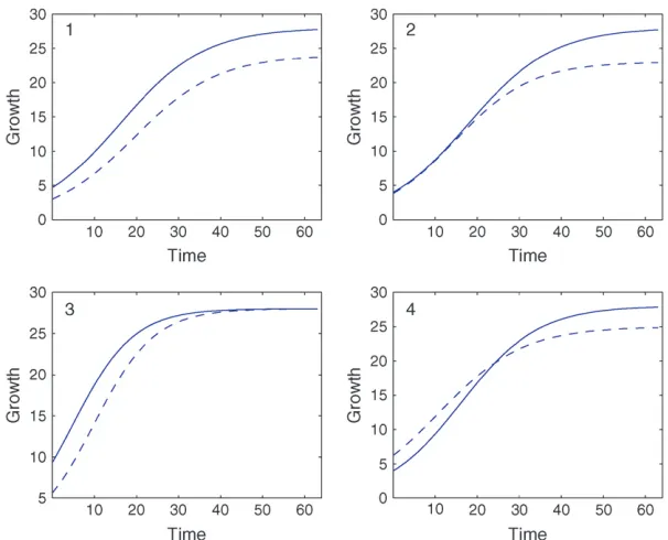
The pattern of the smooth coefficients in the wavelet space resembles the signal pattern in the time space. In Figure 1, c0_{represents a sample of repeated} measure-ments of a logistic growth curve at 12 time points. The smooth coefficients of the first and second Haar wavelet transformation are plotted as c1_and_c2_{, respectively.} The pattern ofc1_and_c2_{coefficients conforms to the} signal pattern although they are in two different resolu-tion levels. Because of the similarity, it is reasonable to model the original growth pattern on the basis of low-dimensional smooth coefficients.

Likelihood of smooth coefficients:Letcj_{be the new} variable with a reduced dimension K (K , T) trans-formed from thejth resolution Haar wavelet. The likeli-hood function based on a mixture model containing two QTL genotypes in the backcross can be rewritten, in terms ofcj_{and marker information}_M_{, as}

LðQjcj; MÞ

¼Y

n

i¼1

½v₁jif1ðc

j i ;w

j

1 ;SjÞ1v2jif2ðc

j i ;w

j

2 ;SjÞ; ð5Þ

where (v1ji, v2ji) are the mixture proportions

corre-sponding to the frequencies of different QTL genotypes for individuali. Because the marker genotype of each individual is known, these mixture proportions actually represent the conditional probabilities expressed in terms of the recombination fractions between the markers and QTL. Q ¼ {vlji, w

j

l , Sj}2l¼1 contains unknown parameters about the QTL position and the mean vector and covariance matrix after the wavelet trans-form, and fl(c

j i ; w

j

l , Sj) is the multivariate normal

distribution of individualithat carries QTL genotypel expressed as

flðc j i ;w

j l ;SjÞ ¼

1

ð2pÞK=2_j_S

jj1=2

3exp 1

2ðc j i w

j l ÞS1jðc

j i w

j l Þ9

;ð6Þ

in whichc_ij¼{cij(k1),. . .,c j

i (kK)} is a vector of smooth

coefficients for individuali,w_lj¼{wlj(k1),. . .,wlj(kK)}

is a vector of expected smooth coefficients for QTL genotypel, andSjis the (K3K) residual covariance

matrix for the smooth coefficients.

Modeling the mean-covariance structures:The tenet of functional mapping is used to model the mean vec-tor wlj by a simple parametric function of biological

(4)

w_l1¼ glðt1;QulÞ1_ffiffiffiglðt2;QulÞ 2

p ;. . .;

glðtT1;QulÞ1glðtT;QulÞ

ffiffiffi

2 p

: ð7Þ

Thus, by estimatingQulwith wavelet-transformed data at an appropriate transformation resolution j, trajectory curves in a time course can be drawn individually for different QTL genotypes. Genotypic differences for the curve can be compared and tested for the statistical significance of genetic control over developmental traits. As shown in functional mapping, the covariance matrixSamong different time points can be modeled using parametric approaches. The structure of the covariance matrix can be modeled by the first-order autoregressive [AR(1)] model (Diggle et al. 2002), expressed as

s2_ð

t1Þ ¼. . .¼s2_ð

tTÞ ¼s2 for the variance

s2ðtt1;tt2Þ ¼s2rjtt2tt1j for the covariance betweentt1andtt2;

ð8Þ

where 0,r,1 is the proportion parameter with which the correlation decays with time lag. The parameters that model the structure of the covariance matrix are arrayed inQv¼(r,s2).

Alternatively, the age-specific change of variance and correlation in the analysis of longitudinal traits can be modeled by Zimmerman and Nu´ n˜ ez-Anto´ n’s (2001) SAD model. Using matrix notation, the error term in regression model (1), ignoring the subscripti, can be expressed as

e¼Ae;

wheree¼{e(t1),. . .,e(tT)}9,e¼{e(t1),. . .,e(tT)}9, and

for the first-order SAD [SAD(1)] model

A¼

1 0 0 0

f 1 0 0

.. .

1 ..

.

ftT1 _ftT2 _ftT3 ₁

0 B B B @

1 C C C A:

The residual covariance matrix of the longitudinal trait is then expressed ( Jaffre´ zicet al. 2003) as

S¼ASeA9; ð9Þ

whereSeis the innovation covariance matrix, expressed

as

Se¼

s2_eðt1Þ 0 0 0

0 s2

eðt1Þ 0 0

.. .

1 ..

.

0 0 0 s2

eðtTÞ 0

B B B B B @

1 C C C C C A :

The time-dependent innovative variances2

e(tt) can be

approached by a polynomial (Pourahmadi 1999) or, for simplicity, is assumed as a constant s2

e. Thus, the

residual matrixScontains the parameters,Qv¼(f,s2e),

that model it.

The residual variances and covariances of the smooth coefficients for the developmental trait measured attT

time points after Wavelet transforms can be derived,

Figure 1.—Smooth coefficients by the Haar wavelet transformation at the first (c1_{) and second resolutions}

(c2_{) follow a similar pattern of}

(5)

with expressions depending on the resolution level of transform. For example, the variance of first-resolution smooth coefficientci1(k1) is expressed as

varðc_i1ðk1ÞÞ ¼var

yiðt1Þ1yiðt2Þ ffiffiffi

2 p

¼1

2ðs

2_ð_t

1Þ1s2ðt2Þ12sðt1;t2ÞÞ;

and the covariance between ci1(k1) andci1(k2) is ex-pressed as

Covðc_i1ðk1Þ;ci1ðk2ÞÞ ¼cov

yiðt1Þ1yiðt2Þ ffiffiffi

2

p ;yiðt3Þ1ffiffiffiyiðt4Þ 2 p

¼1

2ðsðt1;t3Þ1sðt1;t4Þ1sðt2;t3Þ 1sðt2;t4ÞÞ:

Variances and covariances between different time points can be modeled by matrix (Equation 8) for the AR(1) model or by matrix (Equation 9) for the SAD(1) model.

Computational algorithms: We adopt the previous EM algorithm developed on the basis of log-likelihood function (5) (Maet al. 2002; Wuet al. 2004a,b,c) to esti-mate the QTL position in terms of QTL-marker re-combination fractions, the curve parameters (Q_u_l) that model the mean vector, and the parameters (Qv)

model-ing the covariance matrix. In theappendix, a detailed EM algorithm is given to estimate these parameters.

In practice, the QTL position parameter can be viewed as a fixed parameter because a putative QTL can be searched at every 1 or 2 cM on a map interval bracketed by two markers throughout the entire linkage map. The amount of support for a QTL at a particular map position is often displayed graphically through the use of likelihood maps or profiles, which plot the likelihood-ratio test statistic as a function of map posi-tion of the putative QTL.

Thresholding rule:As the noise-free signal is unknown, an approximation of the signal should be sought that is smooth and fits the input well. There are two predomi-nant thresholding schemes for this approximation based on wavelet dimensionality reduction or wavelet shrinkage. One is thehard threshold filter(Hh), or referred to as the ‘‘keep or kill’’ method (Aboufadeland Schlicker1999), that removes coefficients below a threshold value, de-termined by the noise variance. The second is the soft threshold filter (Hs) that shrinks the wavelet coefficients above and below the threshold. Soft thresholding reduces coefficients toward zero (Ghaelet al. 1997). The process of denoising may lose some information in that the denoised signal is irreversibly different from the noisy signal. Thus, thresholding is the cause of this loss of information.

If we desire the resulting signal to be smooth, the soft threshold filter should be used, although the hard

threshold filter performs better. In practice, it is dif-ficult to choose a threshold value. A small threshold value creates a noisy result near the input, while a large threshold value introduces bias. The optimal threshold is somewhere in between.

Many approaches have been available to determine the threshold level. A universal method assigns a thres-hold level equal to the variance times, expressed as

l_n¼pffiffiffiffiffiffiffiffiffiffiffiffiffiffiffi2 logn; ð10Þ

where n is the sample size (Donoho and Johnstone 1994). The hard thresholding rule is defined as

dðy;lÞ ¼ y; ifjyj.l 0; ifjyj,l:

ð11Þ

As pointed out by Donohoand Johnstone(1994) and

Johnstoneand Silverman(1997) that, for a sequence

of normal distributed random variables ziN(0,s2i),

i¼1,. . .,n,

P max

i j

zi s_ij.ln

/0 asn/‘ ð12Þ

so that if a detail coefficient is truly zero then with a high probability it is estimated as zero by the hard thresh-olding rule. The expected number of jzi=sij greater

than the threshold tends to 0. For most applications, the hard thresholding rule keeps only those detail coeffi-cients that are significantly greater than zero. We use the hard thresholding rule as a guidance to either keep or kill the whole level of detail coefficients.

The following procedure is proposed to perform data dimensionality reduction through wavelet transforms:

1. Select proper orthogonal wavelet filters.

2. Calculate the empirical variances for the detail coefficients.

3. Apply the hard thresholding rule to the detail coefficients.

4. Truncate the whole level of the detail coefficients if they are all set to zero by step 3, and keep the whole level of the detail coefficients otherwise.

5. Repeat procedures 1–4 for user prescribed jtimes. Functional QTL mapping will be conducted on the basis of the smooth coefficientscj

if the rest of de-tail coefficients are truncated or on the basis of the smooth coefficientscj11_otherwise.

HYPOTHESIS TESTING

(6)

for wavelet-based functional mapping. The first hypoth-esis test is about the existence of a QTL that affects a longitudinal trait, expressed as

H0: Qu1 ¼Qu2[Qu

H1: At least one of these equalities does not hold:

The test is performed using the log-likelihood ratio (LR) statistics calculated at all given test locations,

LR¼ 2 ln L0ð

˜

Qu;Q˜v:cjÞ

L1ðQˆul;Qˆv:c j_;_M_Þ

" #

; ð13Þ

where L0 andL1 are the corresponding values of the plug-in likelihood values under the null (H0) and the alternative hypothesis (H1). An LR profile is then plotted against test locations throughout the genome. Because the QTL position under the null hypothesis is a nui-sance parameter, the distribution of the LR values un-der H0 is unclear. The critical threshold value can be determined empirically by permutation tests as advo-cated by Churchilland Doerge(1994). Those loca-tions with the LR higher than the threshold value are declared to harbor significant QTL.

Other hypothesis tests after a significant QTL is de-tected include the significance of the additive genetic effect on a certain point or period of growth trajectory during a time course. The wavelet-based parametric model can be used to test the genetic control over particular developmental timing and specific mathe-matical parameters that determine the shape of a curve. Furthermore, wavelet-based functional mapping facili-tates the resolution of fundamental biological issues as follows: (1) If multiple environments are used, as shown in Zhaoet al. (2004b), we can test how the detected QTL interact with the environment in a coordinated manner to determine growth performance at different develop-mental stages; (2) the model can be readily extended to model multiple QTL for growth trajectories throughout the genome and estimate and test the effects of different components of epistasis on growth patterns and forms (Wu et al. 2004a); and (3) wavelet-based parametric functional mapping builds up a bridge between the genetic mechanisms underlying different traits, quanti-tatively testing for the role of pleiotropic QTL on the phenotypic integration of a biological system.

Unlike the test statistic for the QTL significance by Equation 13, the critical threshold values for all the tests after a significant QTL was detected should be determined from simulation studies. However, the null hypotheses for these tests are well nested with their alternative hypotheses and, for this reason, the corre-sponding LR values can be thought to asymptotically follow ax2_{-distribution. Therefore, in theory, the critical} values for these tests can be obtained from thex2_-table,

although the asymptotic properties of these test statis-tics need to be investigated analytically or empirically.

MONTE CARLO SIMULATION

Extensive real data analyses and simulation studies of functional mapping based on parametric modeling have been performed in previous studies (Ma et al. 2002; Wuet al. 2004a,b,c; Zhaoet al. 2004a,b, 2005) to examine its statistical behavior. Here we focus our sim-ulation studies on the comparison between wavelet-based and conventional full-dimensional functional mapping for growth trajectories. Three different dimen-sions of longitudinal data, low (T¼8), intermediate (T¼ 16), and high (T¼64), were simulated to detect the ad-vantage of wavelet-based over conventional approaches when longitudinal data are high dimensional.

We assume a backcross population of a moderately large sample size (200), in which there are two geno-types at each gene. A total of six markers are evenly distributed along a linkage group of length 100 cM. A QTL assumed to affect growth trajectories is located at the center of the linkage group (i.e., 50 cM from either end of the linkage group). By assuming two different QTL genotypic curves, defined byglðtÞ ¼al=ð11blerltÞ,

where al is the genotype-specific asymptotic growth

when time is infinite,blis the genotype-specific

param-eter related to the initial growth, andrlis the

genotype-specific relative growth rate, phenotypic data were simulated using the linear regression model (2), with the time-dependent covariance of residual errors fol-lowing the AR(1) model. The variances2_{was selected} according to the heritability ofH2_¼_{0.1 and 0.4 at the} time point where the genetic variance is in the middle of the largest and the smallest.

It is important to note that the genetic control of a QTL over growth may have different patterns. We consider four such different patterns (Figure 2), as also indicated in Wu and Lin (2006), to investigate how functional mapping affects the estimation of genotypic curves for different patterns. Pattern 1 with two parallel genotypic curves shows that a QTL exerts its effect on the entire process of growth, whereas the other three patterns show the changes of QTL effects over the time course because the two genotypic curves are crossed at a certain point of development. Pattern 2 suggests that a QTL has no effect at an earlier stage of development, but displays an increased influence with time after a particular timing. Pattern 3 is the inverse of pattern B and, thus, reflects the impact of an ‘‘early QTL.’’ The two genotypic curves in pattern 4 make a crossover, suggesting that the underlying QTL alters the direction of its effect. Curve parameters (Qul ¼al;bl;rl) that defined these two patterns are given in Table 1.

(7)

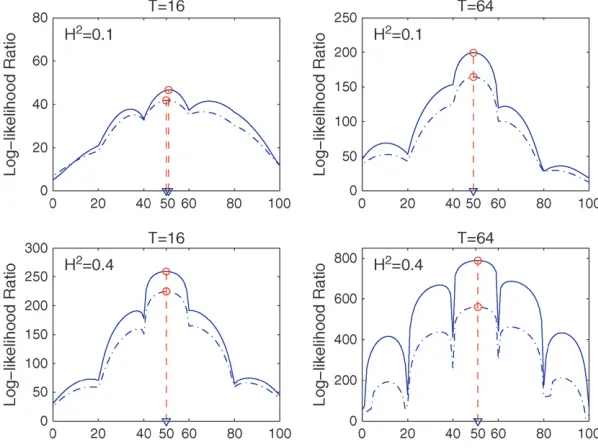
including marker information and longitudinal meas-ures, respectively. According to the thresholding rule, the optimal resolution levels of wavelet transform are 1, 2, and 3 and, therefore, the optimal dimensions after reduction are 4, 4, and 8, for the 8-, 16-, and 64-dimensional longitudinal data, respectively. For each simulation scheme, 200 runs were repeated to estimate the square roots of the mean square errors of the maximum-likelihood estimates (MLEs) of unknown parameters as well as averaged computing times in seconds under the two models. Figure 3 illustrates the profiles of LR values across the simulated linkage group for two different levels of heritability of growth curves (0.1 and 0.4) and of dimension of longitudinal data (16 and 64) calculated from full-dimensional and wavelet-based functional mapping. The peaks of the LR profiles near the center of the linkage group suggest that the two models can provide a good estimate of the QTL location for each simulation scheme.

The two functional mapping models provide compa-rable results; i.e., both of them can be well used to estimate the location of a QTL and QTL genotype-specific parameters that define the shape of growth trajectories (Tables 2–4). As expected, the accuracy and precision of parameter estimation increase when the heritability of growth curves increases from 0.1 to 0.4. The estimation precision of parameters is markedly affected by the dynamic pattern of genetic effects. The QTL location can be estimated with better precision for pattern 3 than for patterns 1, 2, and 4. The estimation precision of all three logistic parameters is better when the dynamic pattern of genetic effects obeys patterns 2 and 3 than patterns 1 and 4. It seems that the estimation precision of the parameters also depends on their types and QTL genotypes. For example, when the dimension of repeated measure is 16, initial growth (b) can be better estimated for QTL genotype 1 under pattern 4 than 1, whereas the converse was true for relative growth

Figure2.—Four different patterns of dynamic genetic effects exerted by a QTL in a backcross design with logistic parameters given in Table 1.

TABLE 1

True logistic parameters for each of the four dynamic patterns of genetic effects as plotted in Figure 2 and the AR(1) parameters modeling the structure of the covariance matrix

Growth pattern

QTL genotype

1 2 AR(1) parameter

a1 b1 r1 a2 b2 r2 r s2a

1 24 7 0.10 28 5 0.1 0.8 0.0200 (0.1199)

2 23 5 0.11 28 6 0.1 0.8 0.0087 (0.0520)

3 28 4 0.14 28 2 0.14 0.8 0.0050 (0.0302)

4 25 3 0.10 28 6 0.11 0.8 0.0181 (0.1089)

a

(8)

(r) rate, although the two patterns have similar estima-tion precision for asymptotic growth (a) (Table 3). The dimension of longitudinal data affects the precision of parameter estimates. Increasing dimensions from an intermediate (16; Table 3) to high level (64; Table 4) can

always improve the estimation precision for all the patterns, but the influence of dimension was pattern specific when the dimensions increase from a low (8; Table 2) to an intermediate level. For patterns 2 and 3, an intermediate dimension provided more precise

Figure _{3.—Log-likelihood ratio (LR) profiles} for the detection of a QTL across a simulated link-age group from a random simulation replicate un-der pattern 1 using full-dimensional (solid curves) and wavelet-based (dashed-dotted curves) func-tional mapping under different levels of heritabil-ity (H2_¼_{0.1 and 0.4) and different longitudinal}

dimensions (T ¼ 16 and 64). The estimated QTL locations are indicated by the arrows.

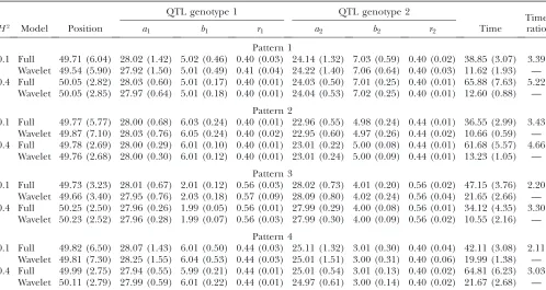
TABLE 2

Means of the MLEs of the QTL position and genotype-specific logistic parameters and the square roots of the mean square errors of the MLEs (in parentheses) for eight-dimensional longitudinal data under different heritability levels

(H2_¼_{0.1 and 0.4) in a backcross from full-dimension parametric and wavelet-based functional}

mapping obtained from 200 Monte Carlo simulations

QTL genotype 1 QTL genotype 2

Time ratio

H2 _Model _Position _a

1 b1 r1 a2 b2 r2 Time

Pattern 1

0.1 Full 50.05 (3.95) 28.00 (1.01) 5.02 (0.26) 0.80 (0.03) 23.97 (0.85) 6.99 (0.35) 0.80 (0.02) 47.81 (3.99) 1.48 Wavelet 50.00 (4.00) 27.93 (1.05) 5.01 (0.26) 0.80 (0.03) 24.04 (0.86) 7.02 (0.35) 0.80 (0.03) 32.31 (1.87) — 0.4 Full 50.21 (2.34) 28.00 (0.37) 5.00 (0.11) 0.80 (0.01) 23.98 (0.34) 7.00 (0.13) 0.80 (0.01) 100.45 (21.97) 1.56

Wavelet 50.17 (2.32) 27.99 (0.39) 4.99 (0.11) 0.80 (0.01) 23.99 (0.34) 7.00 (0.14) 0.80 (0.01) 65.11 (12.71) — Pattern 2

Wavelet 49.77 (3.51) 27.98 (0.46) 6.00 (0.14) 0.80 (0.01) 22.99 (0.35) 4.98 (0.11) 0.88 (0.01) 34.24 (2.72) — Pattern 3

Wavelet 49.87 (2.40) 28.02 (0.38) 2.00 (0.05) 1.12 (0.05) 28.00 (0.35) 4.00 (0.07) 1.12 (0.02) 25.49 (2.54) — Pattern 4

(9)

estimates for growth curve parameters than a low dimension, but, for patterns 1 and 4, the converse was detected.

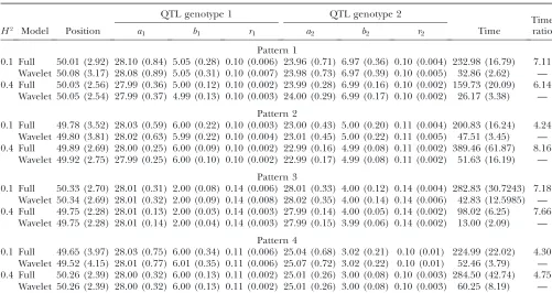
The computing times used for full-dimensional and wavelet-based functional mapping differ notably. The advantage of wavelet-based over full-dimensional func-tional mapping in computing efficiency is consistent for growth curves of different heritabilities and different patterns of dynamic genetic effects. Wavelet-based func-tional mapping is computafunc-tionally more efficient by approximately one to two and two to four times relative to full-dimensional functional mapping when the di-mension of longitudinal data is 8 or 16. This computa-tional efficiency increases to approximately four to eight times when the dimension increases to 64.

DISCUSSION

Genetic mapping has been used as a routine ap-proach to studying the genetic control of complex traits

(Landerand Botstein1989; Zeng1994; Lynchand

Walsh 1998). There is now a pressing need for sta-tistical methods that can unravel the genetic machinery of developmental characteristics because many traits of agricultural, biological, and biomedical interest exhibit

a complex developmental feature. Functional mapping, aimed at characterizing dynamic QTL underlying time-dependent phenotypic differentiation, has emerged as a powerful tool in genetic research (Ma et al. 2002; Wu et al. 2003, 2004a,b,c; Zhao et al. 2004b, 2005;

Macgregoret al. 2005; Yanget al. 2006; reviewed in Wu

and Lin 2006). For a high-dimensional response data set contaminated by noise, the detection of QTL by functional mapping suffers from the so-called ‘‘curse of dimensionality.’’ Also, the complexity and high dimen-sion of longitudinal data make functional mapping computationally prohibitive. In this article, we have incorporated the principle of wavelet shrinkage to map QTL that affect developmental trajectories. As an in-creasingly popular means for data compression and denoising in the context of signal and image process-ing (Donoho and Johnstone 1994; Donoho 1995;

Donohoet al. 1995), wavelet shrinkage can also display

favorable properties to be used for genetic mapping by projecting higher-dimensional data to a manageable lower-dimensional subspace.

The effective use of the wavelet thresholding model for functional mapping can be attributed to three factors. First, the dimensionality of smooth coefficients is only a fraction of the data dimensionality. The curse of

TABLE 3

Means of the MLEs of the QTL position and genotype-specific logistic parameters and the square roots of the mean square errors of the MLEs (in parentheses) for 16-dimensional longitudinal data under different heritability levels

Time ratio

Pattern 1

Wavelet 50.05 (2.85) 27.97 (0.64) 5.01 (0.18) 0.40 (0.01) 24.04 (0.53) 7.02 (0.25) 0.40 (0.01) 12.60 (0.88) — Pattern 2

Wavelet 49.76 (2.68) 28.00 (0.30) 6.01 (0.12) 0.40 (0.01) 23.01 (0.24) 5.00 (0.09) 0.44 (0.01) 13.23 (1.05) — Pattern 3

Wavelet 50.23 (2.52) 27.96 (0.28) 1.99 (0.07) 0.56 (0.03) 27.99 (0.30) 4.00 (0.09) 0.56 (0.02) 10.55 (2.16) — Pattern 4

(10)

dimensionality is removed by considering models for low-dimensional smooth coefficients. Second, the smooth coefficients capture the pattern of the original signal (see Figure 1). As shown in Fan and Lin (1998), the Fourier transformation preserves information content mostly in the low-frequency Fourier coefficients. Like-wise, smooth coefficients are the low-frequency coun-terpart of the signal (Vidakovic1999). Third, removing detail coefficients from the transformation corresponds to removing high-frequency contents of the data, which is equivalent to reducing the noise level and the re-dundancies of the data. Truncating detail coefficients corresponds to a denoising process (Donoho and

Johnstone1994; Donoho1995; Donohoet al. 1995).

By throwing out the noise-rich detail coefficients, the remaining smooth coefficients have a higher signal-to-noise ratio under certain conditions.

We performed simulation studies to investigate the statistical behavior of wavelet-based functional map-ping. The data were simulated for multiple time points using QTL genotype-specific logistic curves, but ana-lyzed by both wavelet-based and full-dimensional func-tional mapping models. The results suggest that the wavelet-based functional mapping outperforms the full-dimensional model in computational efficiency, while

these two models provide consistent results about pa-rameter estimation. With an increased dimension of longitudinal data, the advantage of wavelet-based over full-dimensional functional mapping in computation becomes more pronounced.

The advantage of functional mapping in biology comes from the parametric modeling of the dynamic change of genotypic values for a putative QTL over different time points and the testing of QTL effects on the pattern and form of growth curves on the basis of mathematical parameters that define the curves. Wavelet-based shrinkage has been generally used as a nonpara-metric approach to handle functional data (Morriset al. 2003, 2006; Morris and Carroll2006), thus exhibit-ing a broad use in situations in which no explicit math-ematical function is available to describe longitudinal curves. For many longitudinal trajectories that can be mathematically formulated, such as the sigmoid shape of organismic growth (von Bertalanffy 1957; West et al. 2001), biexponential decay of viral load after med-ical treatment (Hoet al. 1995; Wuand Ding1999), and periodic functions of circadian rhythm (Scheperet al. 1999), a nonparametric treatment will unavoidably re-duce their biological relevance. One of the most sig-nificant relevances of our wavelet-based functional

TABLE 4

Means of the MLEs of the QTL position and genotype-specific logistic parameters and the square roots of the mean square errors of the MLEs (in parentheses) for 64-dimensional longitudinal data under different heritability levels

Time ratio

Pattern 1

Wavelet 50.05 (2.54) 27.99 (0.37) 4.99 (0.13) 0.10 (0.003) 24.00 (0.29) 6.99 (0.17) 0.10 (0.002) 26.17 (3.38) — Pattern 2

Wavelet 49.92 (2.75) 27.99 (0.25) 6.00 (0.10) 0.10 (0.002) 22.99 (0.17) 4.99 (0.08) 0.11 (0.002) 51.63 (16.19) — Pattern 3

Wavelet 49.75 (2.28) 28.01 (0.14) 2.00 (0.04) 0.14 (0.003) 27.99 (0.15) 3.99 (0.06) 0.14 (0.002) 13.00 (2.09) — Pattern 4

(11)

mapping proposed is to preserve all the favorable prop-erties of functional mapping in biologically meaningful hypothesis tests through the integration of wavelet shrinkage within the framework of parametric func-tional mapping.

For a practical data set, the true mean-covariance structures are not known. As shown by Zhaoet al. (2005), different covariance structures may give different results of QTL location estimation. In our simulation studies, the AR(1) model was used to approximate the structure of the covariance matrix. It would be important to model the mean-covariance structures for the time–space data set using different approaches (see Pourahmadi1999, 2000; Panand Mackenzie2003; Wuand Pourahmadi 2003) and further derive dimensionally reduced models at different resolutions.

The wavelet dimensionality reduction method pro-posed in this article has power to map and identify QTL responsible for high-dimensional longitudinal traits. It opens a new avenue to draw a detailed picture of the genetic architecture of a complex biological system by dissecting it into different components and develop-mental stages and studying the genetic regulation and interactions of different QTL involved in various se-quential steps of development. As a starting point, we hope to develop more sophisticated wavelet-based func-tional mapping to take into account the complexity and high dimension of longitudinal data that are needed to describe a biological system in a comprehensive way.

We thank Bruce Walsh for his encouragement to develop this wavelet-based functional mapping model and several anonymous referees for their constructive comments on the earlier versions of this manuscript. The preparation of this work was partially supported by a National Science Foundation grant (0540745), a National Institutes of Health grant (R01 NS041670), and grants from the National Natural Science Foundation of China (09-95671 and 30230300).

LITERATURE CITED

Aboufadel_{, E., and S. S}chlicker_{, 1999} _{Discovering Wavelets. John} Wiley & Sons, New York.

Churchill_{, G. A., and D. W. D}oerge_{, 1994} _{Empirical threshold}

val-ues for quantitative trait mapping. Genetics138:963–971.

Diggle_{, P. J., P. H}eagerty_{, K. Y. L}iang_{and S. L. Z}eger_{, 2002} Anal-ysis of Longitudinal Data. Oxford University Press, Oxford. Donoho_{, D. L., 1995} _{De-noising by soft-thresholding. IEEE Trans.}

Inform. Theory41:613–627.

Donoho, D. L., and I. M. Johnstone, 1994 Ideal spatial adaptation

by wavelet shrinkage. Biometrika81:425–455.

Donoho, D. L., I. M. Johnstone, G. Kerkyacharianand D. Picard,

1995 Wavelet shrinkage: Asymptopia? J. R. Stat. Soc. B 57:

301–369.

Fan_{, J. Q., and S. K. L}in_{, 1998} _{Test of significance when data are}

curves. J. Am. Stat. Assoc.93:1007–1021.

Ghael_{, S. P., A. M. S}ayeed_{and R. G. B}araniuk_{, 1997} _Improved

wavelet denoising via empirical Wiener filtering. Proceedings of SPIE: Wavelet Applications in Signal and Imaging, San Diego, Vol. 3169, pp. 389–399.

Ho_{, D. D., A. U. N}eumann_{, A. S. P}erelson_{, W. C}hen_{, J. M L}eonard

et al., 1995 Rapid turnover of plasma virions and CD4

lympho-cytes in HIV-1 infection. Nature373:123–126.

Jaffre´ zic, F., R. Thompsonand W. G. Hill, 2003 Structured ante-dependence models for genetic analysis of repeated measures on

multiple quantitative traits. Genet. Res.82:55–65.

Jensen, A., and A. laCour-Harbo, 2001 Ripples in Mathematics. Springer, New York.

Johnstone, I. M., and B. W. Silverman, 1997 Wavelet threshold es-timators for data with correlated noise. J. Roy. Stat. Soc. Ser. B59:

319–351.

Lander, E. S., and D. Botstein, 1989 Mapping Mendelian factors underlying quantitative traits using RFLP linkage maps. Genetics

121:185–199.

Lynch_{, M., and B. W}alsh_{, 1998} _{Genetics and Analysis of Quantitative}

Traits. Sinauer, Sunderland, MA.

Ma, C. X., G. Casellaand R. L. Wu, 2002 Functional mapping of

quantitative trait loci underlying the character process: a

theoret-ical framework. Genetics161:1751–1762.

Macgregor_{, S., S. A. K}nott_{, I. W}hite _{and P. M. V}isscher_,

2005 Quantitative trait locus analysis of longitudinal

quan-titative trait data in complex pedigrees. Genetics 171: 1365–

1376.

Mallat, S. G., 1989 A theory for multiresolution signal decomposi-tion: the wavelet representation. IEEE Trans. Patt. Anal. Machine

Intell.11:674–693.

Mallat, S., 1998 A Wavelet Tour of Signal Processing. Academic Press, New York/London/San Diego.

Morris, J. S., and R. J. Carroll, 2006 Wavelet-based functional

mixed models. J. R. Stat. Soc. Ser. B68:179–199.

Morris, J. S., M. Vannucci, P. J. Brown and R. J. Carroll,

2003 Wavelet-based nonparametric modeling of hierarchical

functions in colon carcinogenesis. J. Am. Stat. Assoc.98:573–

597.

Morris_{, J. S., S. A}rroyo_{, B. A. C}oull_{, L. M. R}yan_{, R. H}errick_{et al.,}

2006 Using wavelet-based functional mixed models to

charac-terize population heterogeneity in accelerometer profiles: a case

study. J. Am. Stat. Assoc.101:1352–1364.

Nu´ n˜ ez-Anto´ n, V., and D. L. Zimmerman, 2000 Modeling

non-stationary longitudinal data. Biometrics56:699–705.

Pan, J. X., and G. Mackenzie, 2003 On modelling mean-covariance

structures in longitudinal studies. Biometrika90:239–244.

Pourahmadi_{, M., 1999} _{Joint mean-covariance models with} appli-cations to longitudinal data: unconstrained parameterisation.

Biometrika86:677–690.

Pourahmadi, M., 2000 Maximum likelihood estimation of general-ised linear models for multivariate normal covariance matrix.

Biometrika87:425–435.

Scheper, T. O., D. Klinkenberg, C. Pennartz and J.van Pelt,

1999 A mathematical model for the intracellular circadian

rhythm generator. J. Neurosci.19:40–47.

Sy, J. P., J. M. Taylorand W. G. Cumberland, 1997 A stochastic

model for the analysis of bivariate longitudinal AIDS data.

Biometrics53:542–555.

Vidakovic_{, B., 1999} _{Statistical Modeling by Wavelets. Wiley, New York.} von Bertalanffy, L., 1957 Quantitative laws in metabolism and

growth. Q. Rev. Biol.32:217–231.

Walker, J. S., 1999 A Primer on Wavelets for Their Scientific Applications. Chapman & Hall/CRC, London/New York/Cleveland/Boca Raton, FL.

West, G. B., J. H. Brownand B. J. Enquist, 2001 A general model

for ontogenetic growth. Nature413:628–631.

Wu, H., and A. Ding, 1999 Population HIV-1 dynamics in vivo:

ap-plicable models and inferential tools for virological data from

AIDS clinical trials. Biometrics55:410–418.

Wu, R. L., and M. Lin, 2006 Functional mapping—how to map and

study the genetic architecture of dynamic complex traits. Nat.

Rev. Genet.7:229–237.

Wu, R. L., C.-X. Ma, W. Zhaoand G. Casella, 2003 Functional

map-ping of quantitative trait loci underlying growth rates: a

paramet-ric model. Physiol. Genomics14:241–249.

Wu_{, R. L., C.-X. M}a_{, M. L}in_{and G. C}asella_{, 2004a} _{A general} frame-work for analyzing the genetic architecture of developmental

characteristics. Genetics166:1541–1551.

Wu_{, R. L., C.-X. M}a_{, M. L}in_{, Z. H. W}ang _{and G. C}asella_,

2004b Functional mapping of quantitative trait loci underlying

growth trajectories using a transform-both-sides logistic model.

(12)

Wu, R. L., Z. H. Wang, W. Zhaoand J. M. Cheverud, 2004c A mech-anistic model for genetic machinery of ontogenetic growth.

Genetics168:2383–2394.

Wu_{, W. B., and M. P}ourahmadi_{, 2003} _{Nonparametric estimation of large}

covariance matrices of longitudinal data. Biometrika90:831–844.

Yang_{, R. Q., Q. T}ian_{and S. Z. X}u_{, 2006} _{Mapping quantitative trait}

loci for longitudinal traits in line crosses. Genetics173:2339–2356.

Zeng, Z.-B., 1994 Precision mapping of quantitative trait loci.

Genetics136:1457–1468.

Zhao, W., R. L. Wu, C.-X. Maand G. Casella, 2004a A fast algorithm

for functional mapping of complex traits. Genetics167:2133–2137.

Zhao, W., C.-X. Ma, M. Cheverudand R. L. Wu, 2004b A unifying

statistical model for QTL mapping of genotype3sex

interac-tion for developmental trajectories. Physiol. Genomics 19:

218–227.

Zhao, W., Y. Q. Chen, G. Casella, J. M. Cheverudand R. L Wu,

2005 A nonstationary model for functional mapping of

com-plex traits. Bioinformatics21:2469–2477.

Zimmerman, D. L., and V. Nu´ n˜ ez-Anto´ n, 2001 Parametric

model-ing of growth curve data: an overview. Test10:1–73.

Communicating editor: J. B. Walsh

APPENDIX

In what follows, we provide the EM algorithm for estimating genotype-specific curve parametersQul ¼ ðal;bl;rlÞ(l¼ 1, 2) for the logistic equation of growth trajectories and the covariance parametersQv¼(r,s2) based on the AR(1)

model from wavelet-based functional mapping. The observed log-likelihood function of Equation 5 is rewritten as

logLðQjcj;MÞ ¼X

n

i¼1

log v₁jið2pÞðK=2ÞjSjjð1=2Þexp

1 2ðc

j i w

j 1 Þ9S

1

jðc

j i w

j 1 Þ

1v₂jið2pÞðK=2ÞjSjjð1=2Þexp

1 2ðc

j i w

j 2 Þ9S1jðc

j i w

j 2 Þ

;

where

w11¼

a1=ð11b1er1t1Þ1a1=ð11b1er1t2Þ

ffiffiffi

2

p ;a1=ð11b1e

r1t3_Þ₁_a

1=ð11b1er1t4Þ

ffiffiffi

2

p ;. . .;a1=ð11b1e

r1tT1_Þ₁_a

1=ð11b1er1tTÞ

ffiffiffi

2 p

₉

w₂1¼ a2=ð11b2e

r2t1_Þ₁_a

2=ð11b2er2t2Þ

ffiffiffi

2

p ;a2=ð11b2e

r2t3_Þ₁_a

2=ð11b2er2t4Þ

ffiffiffi

2

p ;. . .;a2=ð11b2e

r2tT1_Þ₁_a

2=ð11b2er2tTÞ

ffiffiffi 2 p ₉ .. . ¼...

untilw1jandw j

2 are determined according to the thresholding rule.

Assuming that QTL genotypes (Q) for each individual are known,i.e., there are no missing data, we construct the complete log-likelihood function as

logLcðQjcj;M;QÞ ¼ Xn

i¼1

log ð2pÞðK=2Þ_j

Sjjð1=2Þexp

1 2ðc

j i jiw

j

1 ð1jiÞw

j 2 Þ9

3S1_jðc_ijj_iw₁j ð1j_iÞw₂jÞ

¼ nK

2 logð2pÞ n

2logjSjj 1 2

Xn

i¼1

ðcijw

j 1 Þ9S1jðc

j i w

j 1 Þ h i j_i 1 2 Xn

i¼1

ðcijw

j 2 Þ9S1jðc

j i w

j 2 Þ

h i

ð1j_iÞ;

wherej1is the indicator variable for a QTL genotype of individualias defined before.

In the E-step of the EM algorithm, we need to calculate the conditional expectation of the complete log-likelihood given the observed data and the current estimation of parameters,

EðlogLcðQjcj;M;QÞÞ ¼

nK

2 logð2pÞ n

2logjSjj 1 2

Xn

i¼1

ðc_i jw₁jÞ9S1_jðc_ijw₁jÞ

h i

Eiðj_iÞ

1

2

Xn

i¼1

ðc_ijw₂jÞ9S1jðc

j i w

j 2 Þ

h i

(13)

where, E() and Ei() denote the conditional expectations given the observed data and current estimation of

parameters.

So, we define the E-step by expressing the posterior probabilities of individualito be QTL genotype 1 or 2 as

EiðjiÞ ¼V1ji¼

v1jið2pÞðK=2ÞjSjjð1=2Þexpð1=2Þðc j i w

j 1 Þ9S1jðc

j i w

j 1 Þ

h i

v1jið2pÞðK=2ÞjSjjð1=2Þexpð1=2Þðcijw j

1Þ9Sj1ðc

j i w

j 1Þ

h i

1v2jið2pÞðK=2ÞjSjjð1=2Þexpð1=2Þðcijw j

2 Þ9Sj1ðc

j i w

j 2Þ

h i

Eið1jiÞ ¼V2ji¼

v1jið2pÞ K

2_j_S

jj

1 2_exp 1

2ðc

j i w

j 2Þ9S1jðc

j i w

j 2Þ

h i

v1jið2pÞðK=2ÞjSjjð1=2Þexpð1=2Þðcijw j

1Þ9Sj1ðc

j i w

j 1 Þ

h i

1v2jið2pÞðK=2ÞjSjjð1=2Þexpð1=2Þðcijw j

2Þ9Sj1ðc

j i w

j 2 Þ

h i:

The M-step is derived by solving the log-likelihood equations of the expected complete log-likelihood function given the observed data and current estimations,

0¼@EðlogLcÞ

@al

¼X

n

i¼1

V_l_j_iðcijw

j l Þ9S

1

j @wlj

@al ;

0¼@EðlogLcÞ

@bl

¼X

n

i¼1 V_ljiðc

j i w

j l Þ9S

1

j @w_lj

@bl ;

0¼@EðlogLcÞ

@rl

¼X

n

i¼1 V_ljiðc

j i w

j l Þ9S1j

@w_lj @rl

;

0¼@EðlogLcÞ

@r ¼

nðK1Þr

1r2

1 2s2_ð₁_r2_Þ2

Xn

i¼1 X2

l¼1 V_ljiðc

j i w

j

l Þ9ð2rA1ð1r2ÞBÞðc

j i w

j l Þ

h i

0¼@EðlogLcÞ

@s2 ¼

nK 2s21

1 2s4ð1r2Þ

Xn

i¼1 X2

l¼1

½V_l_j_iðci jw

j l Þ9Aðc

j i w

j l Þ;

A¼s2_ð₁_r2_Þ_S1

j

B1¼

0 1 0 . . . 0 0 1 0 1 . . . 0 0 0 1 0 . . . 0 0

.. . .. . .. . . . . ... ...

0 0 0 . . . 1 0

2 6 6 6 6 6 6 4 3 7 7 7 7 7 7 5

B2¼diagf0;2;. . .;2;0g

andB¼ ð@A=@rÞ ¼B11rB2.

(14)

solve these equations numerically. For an illustration, we show only the method for computingb1. Thezth step in the Newton–Raphson algorithm is expressed as

b1fzg¼b

fz1g

1

@2EðlogLcÞ @b₁2

1 _@

EðlogLcÞ @b1

" #

j

_b₁¼bf1z1g

: