ABSTRACT
HERMAN, AARON PAUL. Positive Root Bounds and Root Separation Bounds. (Under the direction of Hoon Hong.)
Positive Root Bounds and Root Separation Bounds
by
Aaron Paul Herman
A dissertation submitted to the Graduate Faculty of North Carolina State University
in partial fulfillment of the requirements for the Degree of
Doctor of Philosophy
Applied Mathematics
Raleigh, North Carolina 2015
APPROVED BY:
Erich Kaltofen Seth Sullivant
Agnes Szanto Elias Tsigaridas
Hoon Hong
DEDICATION
BIOGRAPHY
ACKNOWLEDGEMENTS
Special thanks to
• My advisor, Hoon Hong, for teaching me how to think. And, even more impressively, how to slow down.
• Elias Tsigaridas, for helping me have an adventure.
TABLE OF CONTENTS
LIST OF FIGURES . . . vi
Chapter 1 Introduction . . . 1
Chapter 2 Background. . . 4
2.1 Positive Root Bounds of Univariate Polynomials . . . 4
2.1.1 Derivation of the Hong Bound . . . 6
2.1.2 Computing the Hong Bound in Linear Time . . . 9
2.2 Root Separation Bounds of Univariate Polynomials . . . 18
2.2.1 Derivation of the Mahler-Mignotte Bound . . . 19
2.3 Root Separation Bounds of Polynomial Systems . . . 25
2.3.1 Derivation of the Emiris-Mourrain-Tsigaridas Bound . . . 26
Chapter 3 Positive Root Bounds of Univariate Polynomials . . . 33
3.1 Main Results . . . 34
3.2 Proof of Theorem “Over-Estimation is unbounded” . . . 37
3.3 Proof of Theorem “Over-Estimation when Descartes Rule of Signs is exact” . . . 40
3.4 Proof of Theorem “Over-Estimation when there is a single sign variation” . . . . 42
3.A Root of witness polynomials approaches 1/2 . . . 45
3.B Average relative over-estimation for polynomials with single sign variation . . . . 47
3.C Relative over-estimation when the number of sign variations is not equal to the number of positive roots . . . 48
Chapter 4 Root Separation Bounds of Univariate Polynomials . . . 54
4.1 Challenge . . . 55
4.2 Main Result . . . 57
4.3 Derivation . . . 60
4.3.1 Overall framework . . . 60
4.3.2 Derivation of New Univariate Bound . . . 63
4.4 Performance . . . 72
Chapter 5 Root Separation Bounds of Polynomial Systems . . . 74
5.1 Main Result . . . 75
5.2 Derivation . . . 78
5.2.1 Overall framework . . . 78
5.2.2 Derivation of New Multivariate Bound . . . 82
5.3 Performance . . . 92
LIST OF FIGURES
Figure 1.1 Roots of f(x). The largest positive root is highlighted. . . 1
Figure 1.2 Roots of f(x) (left), distances between roots (center), minimum separation highlighted (right) . . . 3
Figure 2.1 Roots of f(x). The largest positive root is highlighted. . . 5
Figure 2.2 All positive and negative points (left), computation of s4 (middle), compu-tation of s0 (right) . . . 10
Figure 2.3 Computation of H(f) . . . 12
Figure 2.4 Roots of f(x) (left), distances between roots (center), minimum separation highlighted (right) . . . 18
Figure 2.5 The curves f1 = 0 and f2 = 0 (Left), the roots of F (center), with root separation highlighted (right). . . 25
Figure 2.6 Not a separating element (left), separating element (right) . . . 28
Figure 3.1 Plot of fc forb= 5 andc= 1 (left), c=.5 (middle), c=.2 (right) . . . 37
Figure 3.2 Average value of RBH(f) for fixed sign change location . . . 47
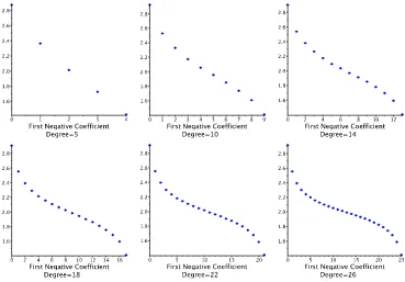
Figure 3.3 RBH(g26,k) for k= 0, . . . ,25 . . . 48
Figure 3.4 Plot offc (red) and gc (blue) ford=k= 3 andc=.3 (left),c=.2 (middle), c=.05 (right). . . 49
Figure 3.5 Plot of fc (red) and gc (blue) with appropriately chosen (c) for d =k = 4 and c=.3 (left), c=.2 (middle), c=.1 (right). . . 51
Figure 4.1 BM M(f(x/s) ) . . . 56
Figure 4.2 Scaling covariance of BN ew,∞ . . . 59
Figure 4.3 Scaled bound for BM M,2 and f. . . 61
Figure 4.4 Average Improvement for given B−Height and Degree 4 . . . 73
Figure 4.5 Improvement for Mignotte Polynomials . . . 73
Figure 5.1 Scaling covariance of BN ew . . . 78
Figure 5.2 Root Separation of F and Root Separation of F(2) . . . 79
Figure 5.3 Scaled bound for BEM T andF. . . 80
Chapter 1
Introduction
In this thesis, we study two classes of bounds on the roots of a polynomial (or polynomial system). A positive root bound of a polynomial is an upper bound on the largest positive root. A root separation bound of a polynomial is a lower bound on the distance between the roots. Both classes of bounds are fundamental tools in computer algebra and computational real algebraic geometry, with numerous applications.
We first study positive root bounds. Consider the following example.
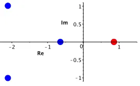
Example 1.1. Letf = 2x4+ 8x3+ 8x2−7x−6. The roots off are plotted in Figure 1.1. The largest positive root of f is .86. Hence, any number greater than or equal to .86 is a positive
root bound.
Figure 1.1: Roots of f(x). The largest positive root is highlighted.
Note that the numbers greater than or equal to .86 are not all of equal quality. In this
first place.
We now consider a well known due to Hong (BH). The value of this positive root bound is BH(f) = 1.63. This bound over-estimates the largest positive root by a factor of 1.9. Clearly,
1.63 is a positive root bound of higher quality than 1×1026. This bound also has an advantage over the exact bound. Unlike the exact bound, the Hong bound can be computed efficiently. So we have a positive root bound that can be computed efficiently and is of very high quality for this polynomial. Could we have known before computing the bound that it would be high quality (or at the very least least, not arbitrarily bad)? We will answer this question in Chapter 3.
Our main concern in Chapter 3 will be the quality of efficiently computable positive root bounds. Higher quality means that the relative over-estimation (the ratio of the bound and the largest positive root) is smaller. We report four findings.
1. Most known positive root bounds can bearbitrarily bad; that is, the relative over-estimation can approach infinity, even when the degree and the coefficient size are fixed.
2. When the number of sign variations is the same as the number of positive roots, the relative over-estimation of a positive root bound due to Hong (BH) is at most linear in
the degree, no matter what the coefficient size is.
3. When the number of sign variations is one, the relative over-estimation of BH is at most constant, in particular 4, no matter what the degree and the coefficient size are.
In the remainder of the thesis, we study root separation bounds. Consider the following example.
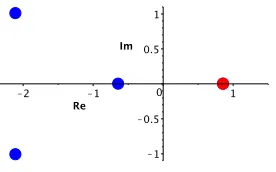
Example 1.2. Let f(x) = x4 −60x3 + 1000x2 −8000x. The roots of f(x) are plotted in
Figure 1.2. The lengths of the red line segments are the distances between the roots of f(x).
The root separation is the smallest of these distances. The root separation of f(x) is √200
(≈14.14), so any number≤√200 is a root separation bound.
As with positive root bounds, not all root separation bounds are of equal quality. For example, 1.00×10−100 is not a very good root separation bound. And also as with positive root
bounds, there exist a root separation bound of perfect quality: √200. But computing the exact root separation is not practical, since the computation of the exact root separation requires the computation of all of the roots of f.
We now consider the well known Mahler-Mignotte bound (BM M). The Mahler-Mignotte
bound can be computed efficiently, and has a similar form to all other known efficiently com-putable root separation bounds. We have
Figure 1.2: Roots of f(x) (left), distances between roots (center), minimum separation
high-lighted (right)
Note that this value is much smaller than the exact root separation bound.
Now consider the polynomial f(x/2 ). Clearly, the roots of f(x/2 ) are the doubled roots
of f. Hence the root separation of f(x/2 ) is doubled. Naturally, we expect a root separation
bound of f(x/2 ) to be doubled as well. Let us see what happens:
BM M(f(x/2) ) = 1.05×10⁻⁶
It is not doubled; in fact, it is smaller! If we triple the roots, it turns out the Mahler-Mignotte bound is even smaller. It appears that the Mahler-Mignotte bound is not compatible with the geometry of the roots off.
It is well known that current root separation bounds are very pessimistic. It is less well known that root separation bounds do not scale correctly (as we see in the above example). So we have a challenge. Namely, we want to find new root separation bounds such that
1. the new bounds are less pessimistic (or almost always less pessimistic) than known bounds 2. the new bounds scale correctly
3. and of course, the new bounds can be computed efficiently.
Chapter 2
Background
This thesis considers three topics: Positive Root Bounds (Chapter 3), Root Separation Bounds of Univariate Polynomials (Chapter 4), and Root Separation Bounds of Polynomial Systems (Chapter 5). In this chapter, we present background material for each topic. For all three topics, we define the category of bounds being considered. We then re-derive previously discovered results that are necessary in later chapters.
2.1
Positive Root Bounds of Univariate Polynomials
In this section, we discuss positive root bounds. A positive root bound of a polynomial is an up-per bound on the largest positive root. Positive root bounds play an important role in computer algebra and computational real algebraic geometry (see [53, 50, 47] for some applications). As a consequence, there has been intensive effort on finding such bounds [30, 10, 2, 27, 49, 2, 3, 22, 6]. First, we formally define a positive root bound. Let f = Pdi=0aixi ∈ R[x] with positive
leading coefficient and at least one positive root. Notation 2.1. x∗(f) = the largest positive root of f.
Definition 2.1. B∈R+ is apositive root bound if B≥x∗(f).
Example 2.1. Consider again the example from the introduction. Let f = 2x4+ 8x3+ 8x2− 7x−6. The roots of f are plotted in Figure 2.1. The largest positive root of f is x∗(f) = .86.
Hence, any number greater than or equal to .86 is a positive root bound.
Some well known positive root bounds are listed below. • Lagrange, 1798 [30]
BL(f) = 1 +
max
q aq<0
aq ad
1
Figure 2.1: Roots of f(x). The largest positive root is highlighted.
wherem= max{q:aq <0}.
• Cauchy, 1829 [10]
BC(f) = max q aq<0
λaq ad
1
d−q
whereλ= #{q :aq<0}.
• Kioustelidis, 1986 [27]
BK(f) = 2 maxq aq<0
aaqd
1
d−q
• Hong, 1998 [22]
BH(f) = 2 maxq aq<0
min
p ap>0
p>q
aqap
1
p−q
Stefanescu, Akritas, Strzebonksi, Vigklas, Batra and Sharma [49, 2, 6] extended the above bounds by splitting single monomials as sums of several monomials and considering different groupings of positive and negative monomials. Batra and Sharma [6] showed that the tightest bound in their framework improves on BH by at most a constant. It is not clear whether a
similar statement holds for the framework in [2], but we have not been able to find a counter example. Complex root bounds (upper bounds on the magnitude of the roots) are by definition positive root bound as well (see [28, 20, 29, 35, 25, 23, 24, 41, 4, 26, 16]).
Of the positive root bounds listed above, the Hong bound will feature most prominently in this thesis. To the best of the author’s knowledge, the Hong bound is the tightest linear complexity positive root bound. It is not obvious that the Hong bound can be computed in linear time, since it involves a max over a min. However, Melhorn and Ray [36] found an ingenious way to compute it in linear time. Their algorithm will be crucial to the complexity results in Chapter 4.
Hong bound using a similar argument to that of Hong in [22]. Then we discuss the algorithm of Melhorn and Ray.
2.1.1 Derivation of the Hong Bound
In this subsection, we re-derive the Hong bound. To the best of the author’s knowledge, every positive root bound is derived using the following strategy:
1. Partition the monomials off into a sum of the form
f =f1+∙ ∙ ∙+fr where every part has the form
fi(x) =apxp+
X
q∈Q aqxq
withaq<0 andq < pfor all q ∈Q.
2. Find a positive root bound for each partition.
3. Define B(f) as the maximum of the positive root bounds derived in Step 2.
We will use this strategy to re-derive the bound of Hong. We will utilize the following Lemma, which was first presented by Kioustelidis in [27].
Lemma 2.1 (Kioustelidis, 1986 [27]). Supposef has the form
f =apxp+
X
q∈Q aqxq
withap >0,aq<0 and q < pfor all q∈Q. Then
f(x)≥0 for all x≥B
where
B = 2 max q∈Q
aq ad
1
d−q
Proof. Let x≥B. We have
f(x) =apxp+X q∈Q
=apxp
1 +X
q∈Q aq ap
xq−p
=apxp
1−X q∈Q
aq ap xq−p
=apxp
1−X q∈Q
aq ap
xd−p
≥apxp
1−X q∈Q
aq ap
Bp−q
sincex≥B (2.1)
To complete the proof, we will show that right term in the right hand side of (2.1) is positive. We have
1−X q∈Q
aq ap
Bp−q = 1−
X
q∈Q
aq ap 2 max
q∈Q
aq ap 1
p−q
p−q
= 1−X
q∈Q
aq ap 2p−q max
q∈Q
aq ap
≥1−X
q∈Q
max
q∈Q
aq ap
2p−q max q∈Q
aq ap
= 1−X
q∈Q
1 2
p−q
≥1−X
q<p
1 2
p−q
≥2−X
q≤p
1 2
p−q
since the summand is 1 when q =p
>2−
∞ X i=0 1 2 i
= 0 (2.2)
Combining (2.1) and (2.2) we have
We have completed the proof of the Lemma.
To derive the Hong bound, we will partition f into a sum of polynomials of the form of
the polynomial in Lemma 2.1. There will be one part for every positive term of f. Negative
monomials will matched with the positive monomial that minimizes
aaqp
1
p−q
, p > q
This choice of partition is motivated by the simple observation that a smaller positive root bound is a tighter positive root bound.
Theorem 2.1 (Hong, 1998 [22]1).
x∗(f)≤BH(f) Proof. Let
μ(q) = arg min p>q
aaqp
1
p−q
Consider the following partition of f:
f = X
p ap>0
fp where fp =apxp+
X
q aq<0
μ(q)=p
aqxq (2.3)
Note that everyfp has the form of the polynomial in Lemma 2.1. Hence
fp(x)≥0 for all x≥Bp (2.4)
where
Bp = 2 maxq aq<0
μ(q)=p
aq ap 1
p−q
= 2 maxq
aq<0
μ(q)=p
aq aμ(q)
1
μ(q)−q
Combining (2.3) and (2.4) we have
f(x)≥0 for all x≥ max p ap>0
Bp (2.5)
1In [22],B
H(f) is derived in a more general setting: absolute positivity of multivariate polynomials. Here we
To complete the proof, we will simplify the right inequality of (2.5). We have
max
p ap>0
Bp= 2 maxp ap>0
max
q aq<0
μ(q)=p
aq aμ(q)
1
μ(q)−q
= 2 max
q aq<0
aaμ(qq)
1
μ(q)−q
= 2 max
q aq<0
min
p ap>0
p>q
aaqp
1
p−q
sinceμ(q) = arg min p>q
aapq
1
p−q
=BH(f) (2.6)
Combining (2.5), (2.6), and the fact that f has positive leading coefficient, we have
x∗(f)≤BH(f)
2.1.2 Computing the Hong Bound in Linear Time
In this subsection, we discuss Melhorn and Ray’s algorithm [36] for computing BH. To derive
the algorithm, they interpret BH geometrically. Then, using a strategy inspired by the Fast
Convex Hull algorithm, they compute BH in O(d) algebraic operations and comparisons.
Consider the following rewrite:
BH(f) = 2H(f), where H(f) = maxq aq<0
min
p ap>0
p>q
aqap
1
p−q
We will compute
log (H(f)) = max q aq<0
min
p ap>0
p>q
log(|aq|)−log(|ap|)
p−q = maxq aq<0
min
p ap>0
p>q
bp−bq p−q
where bi =−log(|ai|). The current problem is interpreted as a geometric problem by viewing
(bp −bq)/(p−q) as the slope of the line between the points vp = (p, bp) and vq = (q, bq). We
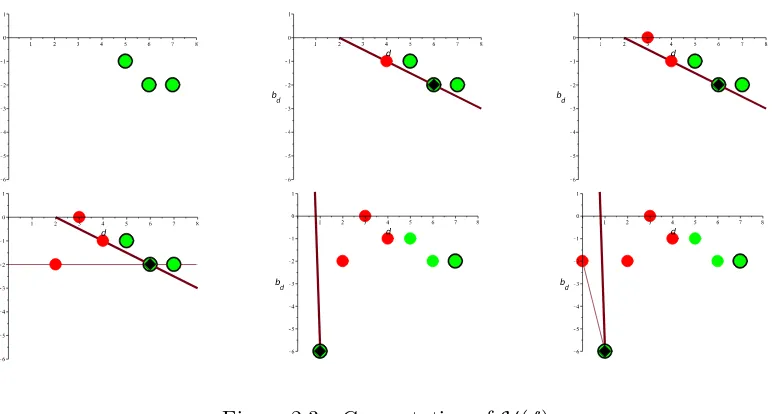
Figure 2.2: All positive and negative points (left), computation of s4 (middle), computation of
s0 (right)
a negative point if ai <0. Under this interpretation, we observe that the quantity
sq = minp ap>0
p>q
bp−bq p−q
is the slope of the tangent line of vq and the set of positive points Pq ={vp :ap > 0, p > q}.
Equivalently,sq is the slope of the tangent line ofvq and theLower Hull ofPq. We want to find
the maximum value ofsq over all of the negative points.
Example 2.2. We illustrate the concepts above with a simple example. Let f = 4x7+ 4x6+ 2x5−2x4−x3−4x2+ 64x−4. The positive points are
(7,−log(4)),(6,−log(4)),(5,−log(2)),(1,−log(64)) = (7,−2),(6,−2),(5,−1),(1,−6)
and the negative points are
(4,−log(2)),(3,−log(1)), (2,−log(4)),(0,−log(4)) = (4,−1),(3,0), (2,−2),(0,−2).
In the left hand plot of Figure 2.2, the positive points are plotted in green and the negative points are plotted in red.
Consider the negative point v4 = (4,−1). The value of s4 is the minimum of the slopes of the lines in the middle plot of Figure 2.2. The line which achieves the minimum slope is highlighted.
Consider the negative point v1 = (0,−2).The value of s0 is the minimum of the slopes of every line between v1 and a positive point. Clearly this minimum is attained by a line between
minimum of the slopes of the two lines.
To compute the quantity log(H(f)) in O(d) algebraic operations and comparisons, we use
an algorithm inspired by the Fast Convex Hull algorithm of computational geometry. At each step of the algorithm, we store and potentially update the following:
sq∗ = the maximum value of sq over the set of negative points L = the lower hull of the set of positive points
We process the points vi from right to left (equivalently: from the points of the highest degree
coefficients to lower degree coefficients).
• If vi is a positive point, we update L using the standard update from the Fast Convex
Hull algorithm.
• Ifvi is a negative point, we update sq∗ (if necessary).
The total work done processing the positive points isO(d), since the Fast Convex Hull algorithm
is O(d)2. It is not obvious that we can process the negative points in a total of O(d) algebraic operations and comparisons. In a naive algorithm, we would calculate si for every negative
point. Furthermore, in a naive calculation of si we would iterate through L starting from the
leftmost (or rightmost) point until we find the point of tangency, then use the point of tangency to calculatesi. This naive strategy would require O(d) operations for every negative point.
To speed up the processing of the negative coefficients, we make the following observations. Observation 2.1. Letvq1 andvq2 be two negative points withq1 < q2. Note that by definition
vq1 lies to the left of vq2 and Pq1 ⊇ Pq2. Let
Lq2 = the Lower Hull ofPq2
Lq1 = the Lower Hull ofPq1
T = the tangent point ofvq2 and Lq2
l= the line from vq2 toT
Then
1. IfT ∈ Lq1 and vq1 lies abovel, then sq1 ≤sq2.
2. IfT ∈ Lq1 and vq1 lies below l, then the tangent point of vq1 and Lq1 lies to the right of
T, and sq1 ≥sq2.
Figure 2.3: Computation of H(f)
3. IfT ∈ L/ q1, then every point to the left of T inLq2 is not in Lq1.
Example 2.3. We illustrate the above observations and the main ideas behind the algorithm
ComputeH with the same example as before. We will process the points from right to left and
at the end of the computation we will have found H(f). We will use Observation 2.1 to avoid
unnecessary computations.
v7: Since v7 is a positive point, we add the point to the (currently empty) lower hull L.
v6: Since v6 is a positive point, we compute the lower hull of L ∪v6. Since the lower hull of two (non vertical) points is simply the same two points, we have L= (v6, v7) .
v5: Sincev5 is a positive point, we compute the lower hull of L ∪v5. We use the standard fast convex hull update. We first set
L= (v5, v6, v7)
then check if we need to delete points from L. We consider the first three points of L.
Since a right turn is made on the path v7→v6 →v5, we do not have to delete any points from L. See the top left of Figure 2.3.
v4: Since v4 is a negative point and we have yet to compute a value of sq∗, we compute s4.
To do so we search through L from the left until we find the tangent line with smallest
slope. We store the current maximum sq∗ =s4, the linelwhose slope is s4 (the line from
v3: Since v3 is a negative point, we potentially have to update sq∗. However, v3 lies above
the line l. Hence s3 will clearly be smaller than s4, and there is no need to compute s3 (Observation 2.1.1). See the top right of Figure 2.3.
v2: Sincev2is a negative point, we potentially have to update sq∗. We notice thatv2lies below
l. Hence we cannot use Observation 2.1.1 to avoid the computation of s2. However, we
can use Observation 2.1.2 to speed up the computation. We search through Lto the right
starting at T =v6 to find the value of s3. In this manner, we avoid having to calculate the slope of the line connecting v3 andv5. We note thats2 is larger thans4, hence we set
sq∗=s2 . See the bottom left of Figure 2.3.
v1: Since v1 is a positive point, we update L. We calculate the lower hull of
L ∪v1 = (v5, v6, v7)∪(v1)
We first set
L= (v1, v5, v6, v7)
Then consider the first three points inL. Since a left turn is made on the pathv6→v5 →
v1, we deletev5 fromL. We now have
L= (v1, v6, v7)
Again, we consider the first three points in L. Since a left turn is made on the path
v7 → v6 →v1, we delete v6 from L. Note that T =v6 was deleted from L, as was every point to the left of T in L (in this case, the only point to the left was v5), confirming
Observation 2.1.3.
Since the current tangent point (v6) was deleted from L, we will reset l and T:
T =v1
l= the line from v1 to (0,∞) See the bottom middle of Figure 2.3.
v0: Since v0 is a negative point, we potentially update sq∗. We notice that v0 lies below l.
Hence we cannot use Observation 2.1.1 to avoid the computation of s0. We search for
Finally, all of the points have been processed, and we return sq∗=H(f).
Let us summarize the strategy in the above example. We use Observation 2.1 to efficiently process the points from right to left. For a negative pointvi, we first check ifviabovel. Ifvilies
abovel, then there is no need to calculatesi(Observation 2.1.1). Ifvi lies belowl, we will search
through Lto the right starting at T (Observation 2.1.2). We use the new point of tangency to
calculatesi. Once the point of tangency is found, we set T to be the new point of tangency and l to the line from vi to T. When processing a positive point, we potentially remove T from L.
IfT is removed fromLwe setT to be the left-most point inL. When later negative points are
processed, no iteration to the right in L will traverse an edge that has already been traversed
(Observation 2.1.3). WhenT is reset, we setlto be the line fromT to (0,∞), so that the next
negative point is guaranteed to be below l.
We are now ready to present the algorithm ComputeH (Algorithm 3) and discuss its
com-plexity (Theorem 2.2). We make the crucial observation that no logarithms are necessary for the computation ofH(f). By taking advantage of the simple fact that
log(A)≤log(B)≤A≤B
we can modify the algorithm discussed above to avoid logarithm computations. For the following algorithms:
• We represent points (i,−log(|ai|) with the pair (i,|ai|).
• ForP1 and P2 represented by (p1,|ap1|) and (p2,|ap2|) respectively, let
SP1,P2 =
|ap2|
|ap1|
1
p1−p2
• For P1 and P2 represented by (p1,|ap1|) and (p2,|ap2|) respectively, the line from P1 to
P2 is represented by
Algorithm 1:LowerHullU pdate
Input :L= a list of points which form a lower hull, sorted from left to right. P = a point to the left of L.T = a point inL. l = a line.
Output: (L0,T0, l0) whereL0 = the lower hull of P ∪ L.T0 =T if T ∈ L0. Otherwise
T =P.l0 =lif T ∈ L0. Otherwisel=the line from P to (0,∞). begin
1
L0 ←(P,L); 2
T0 ← T; 3
l0 ←l;
4
P1,P2,P3← the first 3 elements of L0; 5
while size(L0)>2 and S
P1,P2 >SP2,P3// A right hand turn is made on the
6
path P1 → P2 → P3 do
7
RemoveP2 from L0; 8
if P2 =T then 9
T0 ← P;
10
l0 ←the line fromP to (0,∞);
11
P1,P2,P3 ← the first 3 elements of L; 12
end 13
Algorithm 2:T angentP oint
Input :L= a list of points which form a lower hull, sorted from left to right. P = a point to the left of L.
T = a point in L.
Output:T0: The tangent point ofP and the points to the right ofT inL.
begin 1
T0 ← T; 2
if T0 is not the right most point in L then
3
Y ←the point to the right of T0 inL; 4
whileT0 is not the rightmost point in L and S
P,T0 >SP,Y// The slope of the
5
line from P to T0 is greater than the slope of the line from P
to Y
do 6
T0 ← Y;
Algorithm 3:ComputeH
Input :f =Pdi=0aixi∈R[x]
Output:H(f)
begin 1
T ←(d,|ad|);
2
L ←[T];
3
l ←LineT hrough(T, (0,∞) );
4
H ← −∞;
5
fori from d−1 to 0 by −1 do do 6
P ←(i,|ai|);
7
if ai is positive then
8
(L,T, l)←LowerHullU pdate(L,P,T, l);
9
else 10
if SP,l[2]<Sl[1],l[2] // P lies below l 11
then 12
T ←T angentP oint(L,P,T);
13
l ←LineT hrough(P, T);
14
H ←max{H,Sl[1],l[2]}; 15
Remark 2.1. In [36], the point T and linel are not reset when T is removed from L (as we
did when processing v1 in the previous example, and as we do in Algorithm 1). This appears to a minor oversight which we correct here.
Theorem 2.2(Melhorn, Ray, 2010 [36]). BH(f) can be computed inO(d) algebraic operations
and comparisons using
BH(f) = 2∙ComputeH(f) (Algorithm 3)
Proof. We have already argued that that the total number of algebraic operations and com-parisons required to process the positive points is O(d), since the Fast Convex Hull algorithm
requires O(d) algebraic operations and comparisons. We also already argued that no edge can
be traversed twice when processing negative points, due to Observation 2.1.3. In the Fast Con-vex Hull algorithm, O(d) total edges appear in the lower hull. Hence the negative points are
2.2
Root Separation Bounds of Univariate Polynomials
In this section, we discuss root separation bounds of univariate polynomials. The root separa-tion of a polynomial is the minimum distance between every pair of roots. A root separasepara-tion bound is a lower bound on the root separation. Root separation bounds are a fundamental tool in algorithmic mathematics, with numerous applications in science and engineering. For instance, they are employed in the study of topological properties of curves [31], exact geomet-ric computation [32], algebraic number theory [19], sign evaluation of algebraic expressions [8], quantifier elimination [46], and real root isolation [52, 51].
First, we provide a formal definition of a root separation bound. Let f = Pdi=0aixi = adQdi=1
Q(
x−αi)∈C[x].
Notation 2.2. Δ(f) = mini6=j|αi−αj|is the root separation of f.
Definition 2.2. B∈R+ is aroot separation bound if B ≤Δ(f).
Example 2.4. Consider again the example from the introduction. Let f(x) = x4 −60x3+
1000x2−8000x. The roots of f(x) are plotted in Figure 2.4. The lengths of the red line seg-ments are the distances between the roots of f(x). The root separation is the smallest of these
distances. The root separation of f(x) is √200, so any number ≤ √200 is a root separation
bound.
Figure 2.4: Roots of f(x) (left), distances between roots (center), minimum separation
high-lighted (right)
Most root separation bounds are functions of the discriminant and polynomial norms. Definition 2.3. Thediscriminant of f is
dis(f) =a2dd−2Y i6=j
Some well known root separation bounds are listed below.
• Mahler-Mignotte, 1964 [33, 37]
BM M(f) =
p
3|dis(f)| dd/2+1||f||d−1
2 • Rump, 1979 [43]
BRum(f) =
min(1,|ad|)d(ln(d)+1)|dis(f)|
2d−1dd−1||f||d(ln(d)+3) 1
• Mignotte, 1995 [40]
BM ig(f) =
p
6|dis(f)|
dd/2((d−2)(2d−1))1/2||f||d−1 2
• The DM M1 bound [52]3
BDM M1(f) =
|a0|2 p
|dis(f)|
2d(d−1)/2−2||f||d−1 2
There are many more root separation bounds in the literature (see [14, 5, 8, 37, 7, 44, 42, 39, 17] for more examples). Most have a structure similar to the bounds above.
In Chapter 4 of this thesis, we will present a framework for transforming a known root separation bound into a new improved root separation bound. We will choose to transform the Mahler bound. In the remainder of this section, we will re-derive the Mahler-Mignotte bound.
2.2.1 Derivation of the Mahler-Mignotte Bound
In this subsection, we re-derive the Mahler-Mignotte bound. We follow the commonly used convention of combining Mahler’s original result from [33] and a result due to Mignotte [37]. Mignotte derived a bound on the Mahler Measure of a polynomial. This result is combined with Mahler’s root separation bound (which depends on the Mahler measure of a polynomial) to derive a new root separation bound which depends on the discriminant, degree, and norm of a polynomial.
3In [52], anaggregate separation bound is presented. Aggregate separation bounds are generalizations of root
separation bounds. An aggregate separation bound is a lower bound on products of factors of the form |αi−αj|.
Here, we specialize the bound to the case when the product has a single factor. We also generalize the bound to the case whenf has complex coefficients. This is done by using the lower bound |αi| ≥ |a0|/M(f), instead of
Definition 2.4. TheMahler Measure off is
M(f) =|ad| d
Y
i=1
max{1,|αi|}
We first re-derive Mignotte’s bound on the Mahler measure. We require the following Lemma.
Lemma 2.2. Let γ ∈C. Then
||(x+γ)f||2 =|γ| ∙ ||
x+ 1
ˉ
γ
f||2
Proof. Leta−1=ad+1= 0. To prove the claim, we will expand the squares of both sides of the above equation and observe that they are equal. Consider the following chain of equalities:
||(x+γ)f||22=
d+1 X
i=0
|ai−1+γai|2
=
d+1 X
i=0
(ai−1+γai)(ai−1+γai)
=
d+1 X
i=0
(|ai−1|2+γaiai−1+γai−1ai+|γ|2|ai|2) (2.7)
Similarly, we have
|γ|2∙ ||
x+ 1 γ
f||22 =γγ∙ d+1 X i=0 ai−1+
ai γ 2 =γγ∙ d+1 X i=0
ai−1+aγi ai−1+ aγi
=
d+1 X
i=0
(γai−1+ai) (γai−1+ai)
=
d+1 X
i=0
(|γ|2|ai−1|2+γaiai−1+γai−1ai+|ai|2)
=
d+1 X
i=0
Combining (2.7) and (2.8) yields
||(x+γ)f||22=|γ|2∙ ||
x+ 1 γ
f||22
Taking the square root of both sides completes the proof. Theorem 2.3 (Mignotte, 1974 [37]). We have
M(f)≤ ||f||2
Proof. Without loss of generality, suppose that 0 ≤ |α1| ≤ . . .|αk| ≤ 1 < |αk+1 ≤ . . .|αd|.
Define h(x) =Qki=1(x−αi).We have
||f||2 =|ad| ∙ || d
Y
j=k+1
(x−αj)h||2
=|ad||αk+1| ∙ ||
x− 1
αk+1 Yd
j=k+2
(x−αj)h||2 from Lemma 2.2
=|ad||αk+1| ∙ ∙ ∙ |αd| ∙ || d
Y
j=k+1
x− 1 αj
h||2 from Lemma 2
=|ad| d
Y
i=1
max{1,|αi|} ∙ || d
Y
j=k+1
x− 1 αj
h||2
=M(f)∙ || d
Y
j=k+1
x− 1 αj
h||2 (2.9)
Since h is monic, the polynomial Qdj=k+1x−α1
j
his monic as well. Hence
|| d
Y
j=k+1
x− 1 αj
h||2 ≥1 (2.10)
Combining (2.9) and (2.10) yields
M(f)≤ ||f||2 We have completed the proof of the Lemma.
Theorem 2.4 (Mahler, 1964 [33]). We have
Δ(f)≥
p
3|dis(f)| d(d+2)/2M(f)d−1
Proof. Without loss of generality, suppose that |α1 − α2| = Δ(f), with |α1| ≥ |α2|. We will expand the expression for |dis(f)| using the determinant of the Vandermonde matrix of {α1, . . . , αd}.
|dis(f)| |ad|2d−2
=
1 1 ∙ ∙ ∙ 1
α1 α2 ∙ ∙ ∙ αd
... ... ∙ ∙ ∙ ... αd1−1 αd2−1 ∙ ∙ ∙ αdd−1
2
We can subtract the second column from the first without changing the value of the determinant:
|dis(f)| |ad|2d−2
=
0 1 ∙ ∙ ∙ 1
α1−α2 α2 ∙ ∙ ∙ αd
... ... ∙ ∙ ∙ ...
αd1−1−αd2−1 αd2−1 ∙ ∙ ∙ αdd−1
2 Hence
|dis(f)| |ad|2d−2
=|α1−α2|2
q0 1 ∙ ∙ ∙ 1
q1 α2 ∙ ∙ ∙ αd
... ... ∙ ∙ ∙ ... qd−1 αd2−1 ∙ ∙ ∙ αdd−1
2 (2.11)
whereq0= 0 and
qh= αh
1−αh2
α1−α2 =
h−1 X
j=0
αj1αh2−j. (2.12)
Applying Hadamard’s inequality to the right hand side of (2.11), we have
|dis(f)| |ad|2d−2 ≤ |
α1−α2|2(|q0|2+|q1|2+∙ ∙ ∙+|qd−1|2)
d Y i=2 pi (2.13) where pi = d−1 X
j=0
Dividing both sides of (2.13) by M(f)2d−2/|a
d|2d−2 yields |dis(f)|
M(f)2d−2 ≤ |α1−α2|
2(|q0|2+|q1|2+∙ ∙ ∙+|qd−1|2) max{1,|α1|}2d−2
d
Y
i=2
pi
max{1,|αi|}2d−2
(2.14)
Fori= 2, . . . , dwe have
pi
max{1,|αi|}2d−2 =
d−1 X j=0
α2ij
max{1,|αi|}d−1 2 ≤ d−1 X
j=0
1 =d (2.15)
We also have
(|q0|2+|q1|2+∙ ∙ ∙+|qd−1|2) max{1,|α1|}2d−2
=
d−1 X
h=0
max{1,q|hα1|}d−1 2 =
d−1 X h=0
Ph−1
j=0α
j
1αh2−j max{1,|α1|}d−1
2 from (2.12) ≤ d−1 X h=0
h−1 X j=0 1 2
since |α1| ≥ |α2|and h≤d
=
d−1 X
h=0
h2 (2.16)
Combining (2.14),(2.15), and (2.16), we have
|dis(f)|
M(f)2d−2 ≤ |αr−αs| 2dd−1
d−1 X
h=0
h2 (2.17)
Note that
d−1 X
h=0
h2 = d(d−1)(2d−1)
6 <
d3
3 (2.18)
Combining (2.17) and (2.18), we have
|dis(f)|
M(f)2d−2 ≤ |α1−α2|
2dd−1d3
3 =|α1−α2|2dd+2 1 3 Solving for |α1−α2|and recalling that |α1−α2|= Δ(f), we have
Δ(f)≥
p
We now complete the derivation of the Mahler-Mignotte bound. Note that we present a separation bound which has a slightly different form than those at the beginning of this section. The bound in Proposition 2.1 depends on a parameter k≥2, and is a function of thek−norm
of f.
Proposition 2.1. Letk∈R+, k≥2 and
BM M(f) =
p
|dis(f)| ||f||dk−1
Pk(d)
where
Pk(d) =
√
3
dd/2+1(d+ 1)(1
2−1k)(d−1)
Then Δ(f)≥BM M,k.
Proof. When k = 2, we apply Theorem 2.3 to the expression in Theorem 2.4. For k ≥ 2, we
then apply the well known norm inequality
||f||2 ≤(d+ 1)(
1 2−
1
2.3
Root Separation Bounds of Polynomial Systems
In this section, we discuss root separation bounds of polynomial systems. The root separation of a polynomial system is the minimum distance between every pair of roots. A root sepa-ration bound is a lower bound on the root sepasepa-ration. The study of root sepasepa-ration bounds on polynomial systems is more recent than root separation bounds on univariate polynomials. Many applications arise when generalizing algorithms for univariate polynomials; for example, subdivision algorithms of polynomials systems can be analyzed with root separation bounds [18, 34].
First, we will extend the definition of a root separation bound from the previous section to polynomial systems. Let F = (f1, . . . , fn) ∈ Cn[x1, . . . , xn] be a zero dimensional polynomial
system with no multiple roots. Let {αi} denote the roots of F.
Notation 2.3. Δ(F) = mini6=j||αi−αj||2 is the root separation of F. Definition 2.5. B∈R+ is aroot separation bound if B ≤Δ(F). Example 2.5. Let F = (f1, f2), where
f1 =x21+x22−100
f2 =x21−x22−25
The roots of F are plotted in Figure 2.5. Note that the root separation Δ(F) is √150. Hence,
any number less than or equal to √150 is a root separation bound.
Figure 2.5: The curves f1= 0 and f2= 0 (Left), the roots of F (center), with root separation highlighted (right).
• Emiris, Mourrain, and Tsigaridas, 2010 [18] 4
BEM T(F) =
p
|dis(Tf0)|
(Qn
i=1||fi||Mi)D−1
P(d1, . . . , dn, n)
where
P(d1, . . . , dn, n) =
√
3
DD/2+1∙n1/2C∙√D+ 1(n+ 1)DCDQn
i=1 did+in
Mi D−1
Tf0 = the resultant of (f0, f1, . . . , fn) which eliminates {x1, . . . , xn}
f0 = a separating element in the set
u−x1−ix2− ∙ ∙ ∙ −in−1xn: 0≤i≤(n−1)
D
2
Mi =
Y
j6=i dj
C =
(n−1)
D
2
n−1
In Chapter 5 of this thesis, we extend the framework of the previous chapter to transform a known root separation bound on polynomial systems. We will choose to transform the Tsigaridas bound. In the remainder of this section, we re-derive the Emiris-Mourrain-Tsigaridas bound.
2.3.1 Derivation of the Emiris-Mourrain-Tsigaridas Bound
In this section, we re-derive the Emiris-Mourrain-Tsigaridas bound. We will use the following overall strategy:
1. Construct a u−resultant T(u). This is the resultant of F and a specially chosen f0 ∈
C[u, x1, . . . , xn] which eliminates {x1, . . . , xn}We choose f0 so thatT(u) is square-free. 2. Relate the root separation of F and the root separation of T.
3. Apply the Mahler bound to T.
4. Combine steps 2 and 3 to construct the new root separation bound.
In [18], the authors apply the univariate root separation bound DM M1 (Theorem 1 in that paper) in Step 3. Unfortunately Theorem 1 as stated has a slight error; it cannot be applied to
4The bound presented here is a slight modification of the bound in [18]. We perform the modification to
non-integer polynomials. To derive the multivariate root separation bound, we need to apply a univariate root separation bound which can be applied to complex polynomials. One strategy is to modifyDM M1 so that it applies to complex polynomials. Another strategy is to apply a different bound; here, we simply apply BM ah,∞ toT.
Before constructing the u−resultantT(u), we require the following definition.
Definition 2.6. Let f0 =u−r1x1 − ∙ ∙ ∙ −rnxn ∈ C[u, x1, . . . , xn]. We say f0 is a separating
element ofF if the mapping
V(F)→C
β 7→r1β1+∙ ∙ ∙+rnβn
is injective.
If f0 is a separating element of F, then the polynomial T(u) is square-free. We illustrate the definition and square-free property by a simple example.
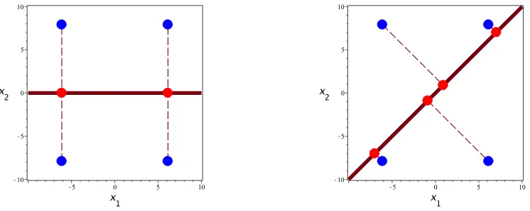
Example 2.6. Let F be the same as in Example 2.5. Consider
f0 =u−x1
In the left plot Figure 2.6, we project every point in R2 onto its x1 coordinate (the red line). The projections of the four roots are the red dots. We can clearly see from this projection that the mappingβ 7→β1 is not injective on the roots of F. Hence f0 is not a separating element of
F. Now consider the u-resultant
T(u) =res(f0, f1, f2) which eliminates x1 and x2
It is simple to verify that T(u) = (2u2−5)2. Clearly this polynomial is not square-free. Hence
any root separation on T(u) will trivially be zero.
Now consider the polynomial
f0 =u−x1−x2
In the right plot of Figure 2.6, we project every point inR2 onto itsx1+x2 value (the red line). The projections of the four roots are the red dots. We can clearly see from this projection that the mappingβ 7→β1+β2 is injective on the roots of F. Hencef0 is a separating element of F. Now consider the same u−resultant construction as before, with the new choice of f0. We have
We compute
dis(T) = 5.76×10¹⁶ 6= 0
Hence T(u) is square-free, and a root separation bound on T(u) will not be trivially 0.
Figure 2.6: Not a separating element (left), separating element (right)
Following [18], we will now present a well known set which has at least one separating element.
Lemma 2.3 (Proposition 6 in [18]). The set
u−x1−ix2− ∙ ∙ ∙ −in−1xn: 0≤i≤(n−1)
D
2
has at least one separating element.
The construction of the set above is motivated by the simple observation that there can be at most (n−1) D2directions (r1, . . . , rn) which yield a non-injective projection. The set is also
chosen so that all polynomials in the set have integer coefficients.
Example 2.7. In the above example, f0 is the element ofF defined by i= 1.
To relate the root separation of F and the univariate polynomialT, we require the
Cauchy-Schwartz inequality.
Lemma 2.5. Letf0 =u−r1x1− ∙ ∙ ∙ −rnxn∈R[u, x1, . . . , xn]. LetTf0(u) denote the resultant
of F and f0 which eliminates x1, . . . , xn. Then
Δ(F)≥ Δ(T) r2
1+∙ ∙ ∙+r2n
1/2
Proof. Let {γ}D
i=1 denote the roots of T. Without loss of generality, assume that
γi =r1αi,1+∙ ∙ ∙+rnαi,n (2.19)
Δ(F) =||α1−α2||2 (2.20)
We have
|γ1−γ2|2=|(r1α1,1+∙ ∙ ∙+rnα1,n)−(r1α2,1+∙ ∙ ∙+rnα2,n)| from (2.19)
=|r1(α1,1−α2,1) +∙ ∙ ∙+rn(α1,n−α2,n)|
≤ r12+∙ ∙ ∙+rn2 (α1,1−α2,1)2+∙ ∙ ∙+ (α1,n−α2,n)2 from Lemma 2.4
= r12+∙ ∙ ∙+rn2||α1−α2||22
= r12+∙ ∙ ∙+rn22Δ(F)2 from (2.20)
Rearranging and solving for Δ(F) yields
Δ(F)≥ |γ1−γ2| r2
1+∙ ∙ ∙+r2n
1/2
≥ Δ(T)
r21+∙ ∙ ∙+r2
n
1/2
We have completed the proof of the Lemma.
Lemma 2.6. Let f0∈ F and Tf0 the resultant of (f0, F) which eliminates x1, . . . , xn. Then
||Tf0||∞≤
n
Y
i=1
||fi||M∞iCD(n+ 1)D n
Y
i=1
n+di di
Mi
Proof. For i= 0, . . . , n,Tf0(u) is homogeneous of degree
d0d1d2. . . di−1di+1∙ ∙ ∙dn=d1d2. . . di−1di+1∙ ∙ ∙dn sinced0 = 1 =Mi
coefficients of (F, f0) with degree D inu. We can write
Tf0(u) =∙ ∙ ∙+ ρkr
D−k k
n
Y
i=1
cMi
i,k
!
∙uk+∙ ∙ ∙ (2.21)
where ρk ∈ Z, cMi,ki is a monomial in the coefficients of fi of total degree Mi, and rkD−k is a
monomial in the coefficients of f0 with total degreeD−k. Since
cMi
i,k =a e1
1 ∙ ∙ ∙aerr
with all aj coefficients offi and e1+∙ ∙ ∙+er=Mi, we have
cMi
i,k = a e1
1 ∙ ∙ ∙aerr ≤ ||fi||e∞1 ∙ ∙ ∙ ||fi||e∞r
= ||fi||e∞1+∙∙∙+rr
= ||fi||Mi
∞
Hence
n
Y
i=1
cMi
i,k ≤ n
Y
i=1
||fi||M∞i (2.22)
Under identical reasoning, we have
|rk|D−k≤ ||f0||D∞−k ≤CD−k (2.23) From Theorem 1.1 of [48], we have
max|ρk| ≤ n
Y
i=0
(# of monomials of degreedi)Mi (2.24)
Sincef0 ∈ F, the number of monomials of degreed0is (n+1). Note also thatM0=d1∙ ∙ ∙dn=D.
Hence
(# of monomials of degree d0)M0 = (n+ 1)D (2.25)
Fori≥0, we have
(# of monomials of degree di)Mi ≤
n+di di
Mi
Combining (2.24), (2.25), and (2.26), we have
max|ρk| ≤(n+ 1)D n
Y
i=1
n+di di
Mi
(2.27)
Now we bound the norm ofTf0. We have
||Tf0||∞= max
0≤k≤D
ρkr
D−k k
n
Y
i=1
cMi
i,k ≤ max
0≤k≤D
ρkr
D−k k
n
Y
i=1
||fi||M∞i
from (2.22) = n Y i=1
||fi||M∞i max
0≤k≤D
ρkrkD−k
≤ n Y i=1
||fi||M∞i max
0≤k≤D
ρkCD−k
from (2.23) = n Y i=1
||fi||M∞iCD max
0≤k≤D|ρk|
≤ n
Y
i=1
||fi||M∞iCD max
0≤k≤D
(n+ 1)
D n
Y
i=1
n+di di Mi from (2.27) = n Y i=1
||fi||M∞iCD(n+ 1)D n
Y
i=1
n+di di
Mi
We have proved the Lemma.
Theorem 2.5 (Emiris, Mourrain, and Tsigaridas, 2010 [18]). Let
B(F) =
p
|dis(Tf0)|
(Qn
i=1||fi||Mi)D−1
P(d1, . . . , dn, n)
where
P(d1, . . . , dn, n) =
√
3
DD/2+1∙n1/2C∙√D+ 1(n+ 1)DCDQn
i=1 did+in
Mi D−1
Tf0 = the resultant of (f0, f1, . . . , fn) which eliminates {x1, . . . , xn}
f0= a separating element in the set
u−x1−ix2− ∙ ∙ ∙ −in−1xn: 0≤i≤(n−1)
D
Mi=
Y
j6=i dj
C=
(n−1)
D
2
n−1
Then Δ(F)≥B(F).
Proof. Clearly, we can write
f0=u−r1x1− ∙ ∙ ∙ −rnxn (2.28)
Since f0∈ F, we have
|rk| ≤C, k = 1∙ ∙ ∙ , n (2.29)
Combining (2.28), (2.29), and Lemma 2.5, we have
Δ(F)≥ Δ(Tf0)
r21+∙ ∙ ∙+r2
n
1/2 ≥
Δ(Tf0)
(n∙C2)1/2 =
Δ(Tf0)
n1/2∙C (2.30) We now apply the bound BM ah,∞ toTf0. Recall that the degree of Tf0 isD. We have
Δ(Tf0)≥BM ah,∞(Tf0)
=
p
3|dis(Tf0)|
DD/2+1√D+ 1D−1||T
f0||
D−1 ∞
≥
p
3|dis(Tf0)|
DD/2+1√D+ 1D−1Qn
i=1||fi||M∞iCD(n+ 1)DQni=1 n+didi
MiD−1
(2.31)
where the last inequality is from Lemma 2.6. Combining (2.30) and (2.31) yields
Δ(F)≥
p
3|dis(Tf0)|
DD/2+1√D+ 1D−1∙n1/2C∙Qn
i=1||fi||
Mi
∞CD(n+ 1)DQni=1 n+didi
MiD−1
= p
|dis(Tf0)|
(Qn
i=1||fi||Mi)D−1
P(d1, . . . , dn, n)
=B(F)
Chapter 3
Positive Root Bounds of Univariate
Polynomials
Introduction
In this chapter, we investigate the quality of known positive root bounds. Of course, every positive root bound over-estimates the largest real root. Higher quality means that the relative over-estimation (the ratio of the positive root bound and the largest positive root) is smaller. We report three findings.
1. We show that most known positive root bounds can bearbitrarily bad; that is, the relative over-estimation can approach infinity, even when the degree and the coefficient size are fixed. A precise statement is given in Theorem 3.1. Contrast this result with similar results on root bounds (upper bounds on the magnitude of the roots): it has been shown that a root bound due to Fujiwara over-estimates the largest magnitude by at most twice the degree [54].
In fact, we prove a more general result: we show that every positive root bound which is also anabsolute positiveness bound (a bound on the largest positive root and the positive roots of the derivatives, see Definition 3.1) can be arbitrarily bad. All positive root bounds listed in Chapter 2 are absolute positiveness bounds, as well as every positive root bound derived in the framework in [6]. It also appears that every positive root bound derived in the framework in [2] is an absolute positiveness bound, although we do not have a proof.
2. We show that when the number of sign variations is the same as the number of positive roots, the relative over-estimation of the Hong Bound (BH) is at mostlinear in the degree,
The motivation for considering number of sign variations is as follows. Theorem 3.1 is a consequence of the fact that for fixed degree and coefficient size, the largest positive root of a polynomial can be arbitrarily smaller than the largest root of its derivatives. Therefore one might wonder if the quality is better when the largest positive root bounds the roots of the derivatives also. One natural case when this happens is when Descartes Rule of Signs is exact (Lemma 3.5).
It is immediate from an example in Theorem 5.3 of [22] that the relative over-estimations
ofBL,BC,andBK (presented in Chapter 2) can approach infinity, even when the degree
is fixed and when the number of sign variations is the same as the number of positive roots. The proof strategy for Theorem 3.2 can be easily adapted to show that the relative over-estimation of every positive root bound in the framework in [6] is at most linear in the degree. It also immediate that there exists at least one positive root bound (namely
BK) in the framework from [2] whose relative over-estimation can approach infinity.
3. We show that when the number of sign variations is one, the relative over-estimation of
BH is at most constant, in particular 4, no matter what the degree and the coefficient
size are. A precise statement is given in Theorem 3.3.
It is again immediate from an example in Theorem 5.3 of [22] that the relative
over-estimations of BL,BC,and BK can approach infinity, even when the degree is fixed and
when the number of sign variations is one. It is not clear if there exists a constant bound on the relative over-estimation for every positive root bound in the framework from [6]. It also immediate that there exists at least one positive root bound (namely BK) in the
framework from [2] whose relative over-estimation can approach infinity.
3.1
Main Results
In this section, we will precisely state the main results of this chapter. Let f =Pdi=0aixi ∈R[x].
We will assume the following throughout the chapter. Assumption 3.1.
1. f has a positive leading coefficient.
2. f has at least one positive root.
Notation 3.1.
||f||= max
0≤i<d−1
|ai| |ad|
V(f) = the number of sign variations of f
C(f) = the number of positive roots of f, counting multiplicities x∗(f) = the largest positive root of f
B(f) = an upper bound on x∗(f) RB(f) =
B(f) x∗(f)
Remark 3.1. From Descartes Rule of Signs, we have V(f) ≥ C(f) and V(f) ≡ C(f) mod 2.
The symbol B stands for a positive root bound. The symbol R stands for “relative
over-estimation”. For every positive root bound B, we obviously have RB(f)≥1.
Definition 3.1 (Absolute positiveness bound [22]). B:R[x]→R+ is anabsolute positiveness
bound if
B(f) ≥ a∗(f)
wherea∗(f) is the threshold of absolute positiveness
a∗(f) = maxnα∈R:∃i∈[0, . . . , d−1] f(i)(α) = 0o
First we show that every absolute positiveness bound can be arbitrarily bad.
Theorem 3.1(Over-Estimation is unbounded). LetB :R[x]→R+be an absolute positiveness bound. Letd≥4 andb >0. Then
sup deg(f)=d
||f||=b
RB(f) =∞
Next we show that when the number of sign variations is equal to the number of positive roots, the relative over-estimation of BH is at most linear in the degree.
Theorem 3.2 (Over-Estimation when Descartes Rule of Signs is exact). We have
sup deg(f)=d
V(f)=C(f)
RBH(f)≤
2d
ln(2)
Theorem 3.3 (Over-Estimation when there is a single sign variation). We have
sup V(f)=1 RBH
(f) = 4
Example 3.1. We will illustrate the result by a simple example.
f =x3+ 9x2−3x−6 V(f) = 1
x∗(f)≈0.94
BH(f) = 2 max
q∈{0,1}p∈{min2,3} aaqp
1
p−q
= 2 max (
min(6 9
1 2−0
,
6 1
1 3−0)
,min
(3 9
1 2−1
,
3 1
1 3−1))
≈1.63 RBH(f) =
B(f)
x∗(f) ≈1.73 Thus we have
RBH(f)≈1.73 ≤ 4,
confirming Theorem 3.3.
Remark 3.2. It turns out that when the sign variation is fixed at 1, the index at which the sign variation occurs affects the average value of the relative over-estimation. We discuss this phenomena in Appendix 3.B.
Remark 3.3. What if the number of sign variations is greater than one and not the same as the number of positive roots? It turns out that the relative over-estimation of every absolute positiveness bound can approach infinity even when the degree is fixed. Precisely, for every absolute positiveness bound B andk >1, one can show that
sup deg(f)=d
V(f)=k
C(f)6=V(f)
RB(f) =∞
3.2
Proof of Theorem “Over-Estimation is unbounded”
In this section, we will prove Theorem 3.1. Let B be an absolute positiveness bound. Let d≥4, b >0 be fixed. We will exploit the following polynomial parameterized by c:
fc =
xd−4(x−c)(x+c) (x−b
2)2+c2
b <4 xd−4(x−c)(x+c)(x−√b)2+c2 b≥4
=
xd−bxd−1+b2
4xd−2+c2bxd−3−c2
b2
4 +c2
xd−4 b <4
xd−2√bxd−1+bxd−2+c22√bxd−3−c2 b+c2xd−4 b≥4
Figure 3.1: Plot offc forb= 5 and c= 1 (left), c=.5 (middle), c=.2 (right)
We will use two key Lemmas. Lemma 3.1. We have
1. fc satisfies Assumption 3.1.
2. deg(fc) =d.
3. ∃c >0 ∀c∈(0, c) ||fc||=b.
Proof. We prove them one by one.
2. Obvious.
3. Suppose b <4. Letc be any positive number such that
c <1 (3.1)
and
c2
b2
4 +c2
< b (3.2)
Such a cexists because the left hand side of (3.2) can be made arbitrarily small for fixed b. Then for allc∈(0, c), we have
||fc||= max
b,b
2
4, c2b, c2
b2
4 +c2
= max
b, c2b, c2
b2
4 +c2
since b 4 <1 = max
b, c2
b2 4 +c2
from (3.1)
=b from (3.2)
Supposeb≥4. Letc be any positive number such that
c <1 (3.3)
and
c2∙(b+c2)< b (3.4)
Such acexists because the right hand side of (3.4) can be made arbitrarily small for fixed b. Then for all 0< c < c, we have
||fc||= max
n
2√b, b, c2∙2√b, c2∙(b+c2)o
= maxn2√b, b, c2∙(b+c2)o from (3.3)
= maxb, c2∙(b+c2) since 2<√b
=b from (3.4)
We have proved the Lemma.
Lemma 3.2. There exists ω >0 such that for allc >0
2. B(fc)≥ω
Proof. We prove them one by one.
1. Obvious.
2. Suppose b <4. Letω = bd andc >0. We have
fc(d−1) = (d)(d−1)∙ ∙ ∙(2)∙x−(d−1)(d−2)∙ ∙ ∙(1)∙b
Hence x∗(fc)(d−1) = db =ω. Since B is an absolute positiveness bound, we have
B(fc)≥x∗(fc)(d−1) =ω
Supposeb≥4. Letω = 2√db and c >0. We have
fc(d−1) = (d)(d−1)∙ ∙ ∙(2)∙x−(d−1)(d−2)∙ ∙ ∙(1)∙2√b
Hence x∗(fc)(d−1) = 2
√
b
d =ω. SinceB is an absolute positiveness bound, we have B(fc)≥x∗(fc)(d−1) =ω
We have proved the Lemma.
Proof of Theorem 3.1. Letc, ω be defined as in Lemmas 3.1 and 3.2. We have
sup deg(f)=d
||f||=b
RB(f) = sup
deg(f)=d
||f||=b B(f) x∗(f)
≥ sup fc
0<c<c B(fc)
x∗(fc) from Lemma 3.1
≥lim c→0
B(fc) x∗(fc) = lim
c→0
B(fc)
c from Lemma 3.2
≥lim c→0
ω
c from Lemma 3.2
=∞
3.3
Proof of Theorem “Over-Estimation when Descartes Rule
of Signs is exact”
In this section, we prove Theorem 3.2. Essentially, we prove Theorem 3.2 by showing that if
V(f) =C(f), then a∗(f) =x∗(f). We then use Theorem 2.3 of [22] to complete the proof. We
break the proof into several Lemmas for clarity. Lemma 3.3. If
V(f) =C(f)
then
V(f0) =C(f0) Proof. From Descartes Rule of Signs
C(f0)≤ V(f0) (3.5)
and
C(f0) =V(f0) mod 2 (3.6)
From repeated application of Rolle’s Theorem, f0 has at least C(f)−1 positive roots. Hence
C(f0)≥ C(f)−1
=V(f)−1 sinceC(f) =V(f) (3.7)
Combining (3.5) and (3.7), we have
V(f)−1≤ C(f0)≤ V(f0) (3.8)
Clearly,
V(f0)≤ V(f) (3.9)
Combining (3.8) and (3.9), we have
V(f)−1≤ C(f0)≤ V(f0)≤ V(f) (3.10)
Combining (3.6) and (3.10), we have
C(f0) =V(f0)
Lemma 3.4. If
V(f) =C(f)
and f0 has a positive root, then
x∗(f0)≤x∗(f)
Proof. Letk =V(f). Without loss of generality, suppose that the positive roots off are ordered
so that
α1≤ ∙ ∙ ∙ ≤ αk
Suppose that x∗(f0) > x∗(f) =αk. We will derive a contradiction. From repeated application
of Rolle’s Theorem, f0 hask−1 roots in the interval [α1, . . . , αk]. Sincef0 has at most k roots
by Descartes Rule of Signs and x∗(f0)> αk,f0 hask roots
β1≤. . . βk−1≤βk
whereβk−1 ≤αk< βk. Since f has positive leading coefficient and αk is the largest root of f,
f is strictly positive on (αk,∞) (3.11)
By identical reasoning
f0 is strictly positive on (βk,∞) (3.12)
Sinceβkis not a double root off0, it follows thatf0 is strictly negative on the interval (βk−1, βk).
In particular,
f0 is strictly negative on the interval (αk, βk) (3.13)
Since f(αk) = 0, from (3.13) we have
f is strictly negative on the interval (αk, βk) (3.14)
Combining (3.11) and (3.14) yields the desired contradiction. We have proved the Lemma.
Lemma 3.5. If C(f) =V(f), then a∗(f) =x∗(f). Proof. Suppose that
V(f) =C(f)
From Lemma 3.3, we have
Hence we can repeatedly apply Lemma 3.4 to show that
x∗(f(r))≤ ∙ ∙ ∙ ≤x∗(f(1))≤x∗(f)
wherer is the largest index such that f(r) has a positive root. Hence
x∗(f) =a∗(f)
We have proved the Lemma.
Proof of Theorem 3.2. From Theorem 2.3 of [22], we have BH(f)
a∗(f) ≤ 2d
ln(2) if deg(f) =d (3.15)
Hence
sup deg(f)=d
V(f)=C(f)
RBH(f) = sup
deg(f)=d
V(f)=C(f)
BH(f) x∗(f)
= sup
deg(f)=d
V(f)=C(f)
BH(f)
a∗(f) from Lemma 3.5
≤ sup
deg(f)=d
V(f)=C(f) 2d
ln(2) from (3.15)
= 2d ln(2) We have proved Theorem 3.2.
3.4
Proof of Theorem “Over-Estimation when there is a single
sign variation”
In this section, we will prove Theorem 3.3. Letfbe a polynomial with positive leading coefficient
and V(f) = 1. Note that ad > 0 and at < 0, where at is the trailing coefficient of f. We will
crucially exploit the following polynomial
g = −xdf
1
x
.
Lemma 3.6. 1
BH(g) ≥
1
4BH(f).
Proof. Repeatedly rewriting g,we have
g = −xdf
1
x
= −xd d
X
i=0
aix−i = d
X
i=0
−aixd−i= d
X
j=0
−ad−jxj = d
X
j=0
bjxj
wherebj =−ad−j. Note thatg has a positive leading coefficient (namely, −at) and at least one
negative coefficient. Recalling the definition of BH, we have
BH(g) = 2 max q bq<0
min
p bp>0
p>q bq bp 1
p−q
= 2 max
q
−ad−q<0
min
p
−ad−p>0
p>q
−
ad−q −ad−p
1
p−q
= 2 max
q ad−q>0
min
p ad−p<0
p>q
ad−q ad−p
1
p−q
For later convenience, we carry out the somewhat unusual re-indexing d−q→pandd−p→q,
obtaining
BH(g) = 2 maxp ap>0
min
q aq<0
d−q>d−p
aapq
1 (d−q)−(d−p)
= 2 max
p ap>0
min
q aq<0
p>q
aapq
1
p−q
SinceV(f) = 1 andf has positive leading coefficient, the conditionp > qis redundant. Dropping
the condition, we have
BH(g) = 2 max p ap>0
min
q aq<0
ap aq 1
p−q
(3.16)
Note that the reciprocal of the maximum of a set of positive numbers is the minimum of the set of the reciprocals. Likewise, the reciprocal of the minimum is the maximum of the reciprocals. Thus we have
1
BH(g)
= 1 2minp
ap>0
max
q aq<0
aaqp
1
p−q
Using the well known min-max inequality, we have
1
BH(g) ≥
1 2maxq
aq<0
min
p ap>0
aq ap 1
p−q
By adding back the redundant the condition p > q, we have
1
BH(g) ≥
1 2maxq
aq<0
min
p ap>0
p>q
aqap
1
p−q
By combining the (3.17) and the definition of BH(f), we finally have
1
BH(g) ≥
1
4BH(f).
We have proved the lemma.
Proof of Theorem 3.3. We will first show that RBH(f) ≤ 4, using the previous Lemma. Note
that the polynomial g has a positive leading coefficient, namely −at. It also has single sign
variation. Thus from [22], we have
RBH(g)≥1 (3.18)
From Descartes’ rule of sign,x∗(f) is the unique positive root off. Likewisex∗(g) is the unique
positive root of g. Thus, we have
1
x∗(g) =x∗(f) (3.19)
By combining Lemma 3.6 and Equations (3.19) and (3.18), we have
RBH(f) =
BH(f) x∗(f) ≤
4/BH(g)
1/x∗(g) = 4
x∗(g) BH(g)
= 4/R(g) ≤ 4.
We will now show that the over-estimation bound is optimal. More precisely, we will show that there exist polynomials with positive leading coefficient, V(f) = 1, and relative
over-estimation arbitrarily close to 4. We will use the following family of polynomials paramterized by d as a “witness” for optimality.
hd(x) =xd+xd−1+∙ ∙ ∙+x−1.
Note that hd has a positive leading coefficient and V(hd) = 1. Since every coefficient of hd is ±1, we have
BH(hd) = 2 (3.20)
It is easy to verify that
lim
d→∞x ∗(h
d) = 1/2 (3.21)
(In Appendix 3.A we include a detailed proof). Combining (3.20) and (3.21), we have
lim
d→∞R(hd) = 2 1/2 = 4