Analysis of Variability in Estimates of Cell Proliferation Parameters for Cyton-Based Models Using CFSE-Based Flow Cytometry

(1)

Analysis of Variability in Estimates of Cell Proliferation Parameters

for Cyton-Based Models Using CFSE-Based Flow Cytometry Data

H.T. Banks, D.F. Kapraun, Kathryn G. Link, and W. Clayton Thompson

Center for Research in Scientific Computation

North Carolina State University, Raleigh, NC 27695-8212

Cristina Peligero, Jordi Argilaguet, and Andreas Meyerhans

ICREA Infection Biology Lab, Department of Experimental and Health Sciences

Universitat Pompeu Fabra, 08003 Barcelona, Spain

November 4, 2013

Abstract

In this article we assess variability in cell proliferation dynamics observed for CD4+ and CD8+ T cells collected from two healthy donors. We review a recently developed class of models that incorporates the so-called “cyton model” for cell numbers into a conservation-based PDE model for cell population dynamics and describe a statistical model that relates CFSE-based flow cytometry data to such models. A parameter estimation scheme is summarized and then applied to a large body of data to assess experi-mental variability (variation in parameter estimates as identical experiments are replicated) and biological variability (differences in parameter estimates obtained for different donors and cell types) in the context of these models. Variability in the data obtained from replicated experiments is also discussed. The results of this study indicate that many of the cyton model parameters for describing cell proliferation can be reliably estimated using our approach; however, they also show that substantial changes to our mathematical model and/or experimental procedures may be required to ensure identifiability of the remaining cell proliferation parameters.

1 Introduction

The adaptive immune response is a major component of the human immune system’s defense against invading pathogens. The adaptive immune system consists of B and T lymphocytes, which recognize invaders by specific cell surface receptors and exert their responses by soluble and cellular effector mechanisms. As the success of this system depends on the lymphocytes’ capacity to proliferate in response to an infection, the ability to accurately predict this behavior in the presence of specific environmental stimuli has important implications for human health research in areas such as the treatment and prevention of infectious disease and immunosuppression for organ and tissue transplants. Such predictions can be made through the use of mathematical models.

(2)

In this study, we consider a mathematical model that incorporates the “cyton model” for cell numbers into a partial differential equation model for cell proliferation dynamics that is based upon the conservation of CFSE mass within a population of proliferating cells. Utilizing a weighted least squares parameter estimation scheme, we fit this model to CFSE-based flow cytometry data obtained for CD4+ and CD8+ T cells collected from two healthy donors. Measurements were made in triplicate on each of five days, making it possible to construct a considerable number of five-day data sets for each donor and cell type. In theory, each such data set should be very similar, so one might expect that a set of parameters for describing cell proliferation dynamics observed in one of the data sets should be essentially equivalent to those describing observations made using another of the data sets. By applying our parameter estimation scheme to each five-day data set, we are able to assess experimental variability in the estimates of the parameters characterizing a specific cyton-based mathematical model. Also, by collecting data from two different human donors and considering two specific cell types, we are able to make some observations concerning biological variablility in the cell proliferation parameters.

2 Data Collection Procedure

As discussed above, the goal of this study is to assess the experimental and biological variability in parameter estimates produced using CFSE-based flow cytometry data and cyton-based mathematical models. To obtain such data, we collected blood samples from two human donors and isolated peripheral blood mononuclear cells (PBMCs) from these samples. The PBMCs (hereafter referred to as just “cells”) were then passed through a strainer to remove clumps of cells and stained with CFSE according to the standard protocol [15]. Forty-five minutes after CFSE staining, the cells were stimulated to divide by exposing them to phytohaemagglutinin (PHA), a nonspecific T cell mitogen. Then, approximately 1 million cells were placed into each of several “wells”, which are typical containers for cell culture experiments. Each well contained approximately 1 mL of RPMI-1640/10% fetal calf serum (FCS), which is a typical nutrient medium for such experiments. For each one of the donors, three wells were “seeded” in this way for each of five measurement times in order to allow for measurements to be obtained in triplicate at each time point; thus, 15 wells were seeded per donor. Since two donors were considered, a total of 30 wells were seeded at the beginning of the experiment.

(3)

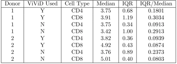
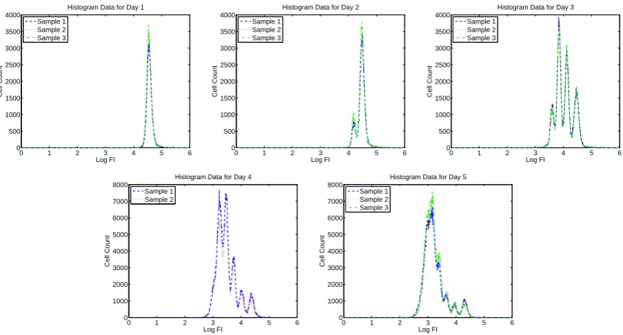
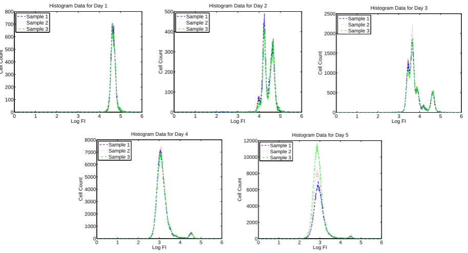
cells acquire more “peaks” as the cells divide asynchronously. In Figures 1 through 8, we present summary histograms for the data collected in our study. Each of these ﬁgures illustrates the preceding point.

As described in the preceding paragraph, the FI emitted in the “CFSE range” by a given cell may be taken to be synonymous with the mass of CFSE contained in that cell. Therefore, CFSE data can be used to validate a mathematical model describing cell population dynamics that is based upon mass conservation principles. Such a model is described in detail in Section 3. Furthermore, when cells have been labeled with other markers (as is the case for the experiments in this study), information about FI at other wavelengths can be used to distinguish between diﬀerent types of cells (e.g., CD4+ versus CD8+ T cells, or living versus dead cells) [15].

In order to ascertain variability in parameters and measured data, we require a considerable number of data sets. To this end, we use various combinations of the triplicate samples collected on Days 1 through 5 to form a large number of time series data sets. Since three samples were collected on each of ﬁve days, there should be 35_{= 243 possible ways to form a ﬁve-day “longitudinal” data set for each donor. However,}

data for one of the samples corresponding to Donor 1 and Day 4 was not available due to an instrument problem; therefore, there are in fact only 34_×_{2 = 162 possible ways to form a ﬁve-day data set for Donor 1.}

It should explicitly noted that data sets formed in this waydo not represent truly longitudinal data because measurements corresponding to each time point were made using distinct cell cultures (wells). In this type

ofin vitro experiment (see, for example, [15], [13], [17], and [2])it is tacitly assumed that the populations of

cells in each well are identical (up until the moment cells are harvested from a particular well) in that they

include the same numbers of total cells in the same proportions (according to cell type). This assumption allows one to interpret time series data sets formed as described above as having come from longitudinal observations. In reality, however, there can be considerable variation in the cell cultures in the various wells due to experimental error in the initial seeding of the wells. This issue will be discussed further in Section 5.

3 Mathematical Model

Here, we summarize a class of models originally proposed in [20] and further developed in [6] and [2]. We then identify the speciﬁc model to be considered for the purposes of our variability study.

3.1 Basic Label-Structured Model for Cell Densities

Letni(t, x) be a structured density (in cells per unit FI), whereiis a whole number representing a speciﬁc “generation” of cells (or number of divisions completed), t denotes the time elapsed (in hr) since some arbitrary starting time, and x denotes FI induced by CFSE. Also, let {αi(t)}, {βi(t)}, and v(t) denote exponential division rates, exponential death rates, and the CFSE exponential decay rate, respectively (all in hr−1). Then the dynamics of a population of cells are described by

∂n0(t, x)

∂t −v(t)

∂[xn0(t, x)]

∂x = −(α0(t) +β0(t))n0(t, x) fori= 0, ∂ni(t, x)

∂t −v(t)

∂[xni(t, x)]

∂x = −(αi(t) +βi(t))ni(t, x) +Ri(t, x) fori≥1,

(3.1)

wherex≥0 and the “recruitment” terms are given by

Ri(t, x) = 4αi−1(t)ni−1(t,2x) (3.2)

fori≥1. The initial conditions are given by

ni(t0, x) =

{

Φ(x) fori= 0,

0 fori≥1, (3.3)

wheret0indicates the time of the ﬁrst observation and Φ(x) is the structured density for cells in the initial

(4)

0 1 2 3 4 5 6 0 500 1000 1500 2000 2500 3000 3500 4000

Histogram Data for Day 1

Log FI

Cell Count

Sample 1 Sample 2 Sample 3

0 1 2 3 4 5 6

0 500 1000 1500 2000 2500 3000 3500 4000

Log FI

Cell Count

0 1 2 3 4 5 6

0 500 1000 1500 2000 2500 3000 3500 4000

Log FI

Cell Count

0 1 2 3 4 5 6

0 1000 2000 3000 4000 5000 6000 7000 8000

Log FI

Cell Count

Sample 1 Sample 2

0 1 2 3 4 5 6

0 1000 2000 3000 4000 5000 6000 7000 8000

Log FI

Cell Count

Figure 1: Summary histogram data for CD4+ T cells measured for Donor 1 using ViViD dye to exclude dead cells.

0 1 2 3 4 5 6

0 200 400 600 800 1000 1200 1400

Log FI

Cell Count

0 1 2 3 4 5 6

0 200 400 600 800 1000 1200 1400 1600 1800

Log FI

Cell Count

0 1 2 3 4 5 6

0 500 1000 1500 2000 2500 3000 3500

Log FI

Cell Count

0 1 2 3 4 5 6

0 1000 2000 3000 4000 5000 6000 7000 8000 9000

Log FI

Cell Count

Sample 1 Sample 2

0 1 2 3 4 5 6

0 2000 4000 6000 8000 10000 12000

Log FI

Cell Count

(5)

0 1 2 3 4 5 6 0 500 1000 1500 2000 2500 3000 3500 4000 4500

Log FI

Cell Count

0 1 2 3 4 5 6

0 500 1000 1500 2000 2500 3000 3500 4000 4500

Log FI

Cell Count

0 1 2 3 4 5 6

0 500 1000 1500 2000 2500 3000 3500 4000 4500

Log FI

Cell Count

0 1 2 3 4 5 6

0 1000 2000 3000 4000 5000 6000 7000 8000 9000

Log FI

Cell Count

Sample 1 Sample 2

0 1 2 3 4 5 6

0 1000 2000 3000 4000 5000 6000 7000 8000

Log FI

Cell Count

Figure 3: Summary histogram data for CD4+ T cells measured for Donor 1 without using ViViD dye to exclude dead cells.

0 1 2 3 4 5 6

0 200 400 600 800 1000 1200 1400

Log FI

Cell Count

0 1 2 3 4 5 6

0 500 1000 1500 2000 2500

Log FI

Cell Count

0 1 2 3 4 5 6

0 500 1000 1500 2000 2500 3000 3500 4000 4500

Log FI

Cell Count

0 1 2 3 4 5 6

0 2000 4000 6000 8000 10000

Log FI

Cell Count

Sample 1 Sample 2

0 1 2 3 4 5 6

0 2000 4000 6000 8000 10000 12000

Log FI

Cell Count

(6)

0 1 2 3 4 5 6 0 500 1000 1500 2000 2500

Log FI

Cell Count

0 1 2 3 4 5 6

0 500 1000 1500 2000

Log FI

Cell Count

0 1 2 3 4 5 6

0 500 1000 1500 2000 2500 3000

Log FI

Cell Count

0 1 2 3 4 5 6

0 1000 2000 3000 4000 5000 6000

Log FI

Cell Count

0 1 2 3 4 5 6

0 1000 2000 3000 4000 5000 6000 7000

Log FI

Cell Count

Figure 5: Summary histogram data for CD4+ T cells measured for Donor 2 using ViViD dye to exclude dead cells.

0 1 2 3 4 5 6

0 100 200 300 400 500 600 700 800

Log FI

Cell Count

0 1 2 3 4 5 6

0 100 200 300 400 500

Log FI

Cell Count

0 1 2 3 4 5 6

0 500 1000 1500 2000 2500

Log FI

Cell Count

0 1 2 3 4 5 6

0 1000 2000 3000 4000 5000 6000 7000 8000

Log FI

Cell Count

0 1 2 3 4 5 6

0 2000 4000 6000 8000 10000 12000

Log FI

Cell Count

(7)

0 1 2 3 4 5 6 0 500 1000 1500 2000 2500 3000

Log FI

Cell Count

0 1 2 3 4 5 6

0 500 1000 1500 2000 2500

Log FI

Cell Count

0 1 2 3 4 5 6

0 500 1000 1500 2000 2500 3000

Log FI

Cell Count

0 1 2 3 4 5 6

0 1000 2000 3000 4000 5000 6000

Log FI

Cell Count

0 1 2 3 4 5 6

0 1000 2000 3000 4000 5000 6000 7000

Log FI

Cell Count

Figure 7: Summary histogram data for CD4+ T cells measured for Donor 2 without using ViViD dye to exclude dead cells.

0 1 2 3 4 5 6

0 100 200 300 400 500 600 700 800

Log FI

Cell Count

0 1 2 3 4 5 6

0 100 200 300 400 500 600

Log FI

Cell Count

0 1 2 3 4 5 6

0 500 1000 1500 2000 2500 3000

Log FI

Cell Count

0 1 2 3 4 5 6

0 1000 2000 3000 4000 5000 6000 7000 8000

Log FI

Cell Count

0 1 2 3 4 5 6

0 2000 4000 6000 8000 10000 12000

Log FI

Cell Count

(8)

Chapter 3 of [20]. We remark here thatt0typically coincides with the time at which the cells were stimulated

to divide, but for the purposes of our experiment the ﬁrst observation actually occurred approximately 24 hours after stimulation. We also mention that the form of the recruitment terms (3.2) assumes an even partitioning of the CFSE in a mother cell between two daughter cells during cytokinesis; i.e.,we assume that

each daughter cell receives exactly one half of the CFSE that was present in the mother cell. Long-standing

results indicate that the partitioning of cytoplasm to two daughter cells during mitosis isnot even [21], and a recent review [9] suggests that incorporating the assumption of asymmetric cell division into mathematical models for cell proliferation will “improve assessment of T cell performance parameters from CFSE-based proliferation assays.” Nevertheless, we follow the convention of earlier work [2, 11, 15, 17, 18, 20] in making the simplifying assumption that CFSE is evenly distributed during cell division.

As proposed in [18], the solutions to the system of partial diﬀerential equations (PDEs) given in (3.1) can be factored as

ni(t, x) =Ni(t)¯ni(t, x),

where Ni(t) indicates the number of cells having completedi divisions at timet and ¯ni(t, x) describes the

distributionof CFSE within that generation of cells at timet; that is, ¯ni(t, x) is a probability density function

(pdf) in the variablex, so that for any ﬁxedt, ¯ni(t, x)≥0 for allxand ∫ _∞

0

¯

ni(t, x)dx= 1.

TheNi’s satisfy the system of ordinary diﬀerential equations (ODEs) given by

dN0(t)

dt = −(α0(t) +β0(t))N0(t) fori= 0, dNi(t)

dt = −(αi(t) +βi(t))Ni(t) + 2αi−1(t)Ni−1(t) fori≥1,

(3.4)

and have initial conditions given by

Ni(t0) =

{

N0=

∫_∞

0 Φ(x)dx fori= 0,

0 fori≥1. (3.5)

Each ¯ni satisﬁes the PDE

∂n¯i(t, x)

∂t −v(t)

∂[x¯ni(t, x)]

∂x = 0 (3.6)

and the initial condition

¯

ni(t0, x) =

2i_Φ(2i_x₎

N0

(3.7)

forx≥0.

It is worth noting that cells will only divide a ﬁnite number of times in the time frame of at typical

in vitro cell culturing experiment. Therefore, we typically compute solutions to (3.4) and (3.6) only for

i∈ {0,1, . . . , imax}, whereimaxis the largest number of divisions we expect a cell from the initial population to undergo during the period of observation. For a ﬁve-day experiment such as that presented in Section 2, it is rare for cells to undergo more than 12 divisions. In order to capture the behavior of all but a negligible number of cells, we use the conservative value ofimax= 16 for our purposes in this variability study.

3.2 Autofluorescence

Thus far, we have described a model that accounts only for FI induced by CFSE, but as noted in [20], the experimentally measured FI of a cell is actually the sum of CFSE-induced FI and the cell’s natural “autofluorescence”. Therefore, following the work of [11], we let ñi(t,x˜) be a structured density (in cells per unit FI), whereiagain denotes a specific generation of cells, t denotes time elapsed (in hr), and ˜xdenotes

measured FI. Here,

˜

(9)

wherexandxa represent the FI due to CFSE and autoﬂuorescence, respectively.

If we assume solutionsni(t, x) to (3.1) and (3.3) have already been computed and thatxais a realization of a random variableXa with pdffXa(xa;t), then the densities ˜ni(t,x˜) can be computed using the convolution

integral [11, 18]

˜

ni(t,x˜) = ∫ _∞

−∞

ni(t, x)fXa(˜x−x;t)dx=

∫ x˜

0

ni(t, x)fXa(˜x−x;t)dx. (3.8)

Under certain assumptions, this convolution integral can be computed quickly and eﬃciently as demonstrated in [11].

3.3 Cyton Model for Cell Numbers

We now turn our attention to the cyton model [12, 13], which is an alternative to (3.4) that arises from two simple assumptions. The ﬁrst, which is self-evident, is that any given cell must eventually either divide or die. The second, which is based upon experimental evidence, is that the processes of cell division and death operate independently of one another [13]. Thus, we can assume that the destiny of any particular cell is governed by two ﬁxed numbers: a “time until division” and a “time until death”. In particular, the actual fate of the cell (division or death) can be determined by observing which of these two numbers is smaller. For individual cells within a population of cells sharing similar characteristics (e.g., cells of the same type having undergone the same number of divisions), it is reasonable to assume that the “time until division” and “time until death” are realizations of independent random variables. These random variables are described by probability distributions, and so the cyton model requires parameters that can be used to uniquely determine the probability distributions for times until division and death of cells in a given population (e.g., CD4+ T cells having undergone 1 division). The authors of [13] chose the term “cyton” to denote the “combination of independent cellular machines governing times to divide and die” and represented a cyton mathematically using a pair of probability density functions. For example, ifϕi andψi are the pdfs for time until division and time until death, respectively, of cells in generation i, then the cyton for generation ican be denoted (ϕi, ψi). One additional consideration is that, in reality, not all cells in a given population will divide if they avoid death (at least not within the time frame of a typical in vitro cell culturing experiment) [13]. Therefore, the cyton model includes the notion of “progressor fraction”: for a given generation of cells, only a certain proportion have the potential to “progress” to the next generation via cell division.

Let Fi denote the progressor fraction for generation i; that is, Fi represents the proportion of cells in generationi that would (eventually) divide in the absence of any possibility of cell death. Then, deﬁne the random variableTdiv

i to be the time required for a cell in generation i (with the potential to progress) to complete its next division (measured in hours since the completion of theith_{division, or in the case of}_Tdiv

0 ,

hours sincet0). Similarly, deﬁne the random variableTidie to be the time required for a cell in generation i to die. Finally, let ϕi(t) andψi(t) be pdfs forTidiv andTidie, respectively. If we deﬁneNi(t) as before, the cyton model is then given by

N0(t) = N0−

∫ t

t0

(

ndiv₀ (s) +ndie₀ (s))ds fori= 0,

Ni(t) = ∫ t

t0

(

2ndiv_i₋₁(s)−ndiv_i (s)−ndie_i (s))ds fori≥1,

(3.9)

where ndiv_i (t) andndie_i (t) are rates (in cells/hr) at which cells in generationi divide and die, respectively. These rates are deﬁned as

ndivi (t) =       

F0N0

( 1−

∫ t

t0

ψ0(s)ds

)

ϕ0(t) fori= 0,

2Fi ∫ t

t0

ndiv_i₋₁(s) (

1− ∫ t−s

0

ψi(ξ)dξ )

ϕi(t−s)ds fori≥1.

(10)

and

ndie_i (t) =       

N0

( 1−F0

∫ t

t0

ϕ0(s)ds

)

ψ0(t) fori= 0,

2 ∫ t

t0

ndivi₋1(s)

( 1−Fi

∫ t−s

0

ϕi(ξ)dξ )

ψi(t−s)ds fori≥1.

(3.11)

There is considerable experimental evidence [7, 12, 13] that supports the cyton model, and it has an advantage over models such as (3.4) in that it directly connects cell population numbers to probablity distributions describing times at which cells in a given generation will divide or die. Identifying these distributions for populations of lymphocytes exposed to speciﬁc environmental stimuli allows for a detailed quantitative description of the adaptive immune response.

3.4 Label-Structured Cyton Model for Cell Densities

As in [2], we incorporate the cyton model for cell numbers into the division- and label-structured model framework described previously by replacing the sink and source terms in the right-hand sides of (3.1) with terms involving the cyton-based rates to obtain

∂n0(t, x)

∂t −v(t)

∂[xn0(t, x)]

∂x = −(n

div

0 (t) +ndie0 (t))¯n0(t, x) fori= 0,

∂ni(t, x)

∂t −v(t)

∂[xni(t, x)]

∂x = (2n

div

i₋1(t)−ndivi (t)−ndiei (t))¯ni(t, x) fori≥1.

(3.12)

Solutions of this system are then given byni(t, x) =Ni(t)¯ni(t, x), where theNi(t)’s satisfy the cyton model equations (3.9) and initial conditions (3.5) and each ¯ni(t, x) satisﬁes (3.6) and (3.7) as before.

Like (3.1), the model given by (3.12) may be properly described as a division- and label-structured population model, as it makes use of structure variables for division number (or generation) i and CFSE label content (which is proportional to CFSE-wavelength FI)x. Also, as described in [11, 18] and summarized in [2], the factorable form of the solutions{ni(t, x)}and the technique for converting these to corresponding solutions{n˜i(t,x˜)}via convolution integrals (cf. (3.8)) makes it possible to obtain numerical solutions very quickly when the model parameters are given [2, 11]. This model has been shown to yield a reasonably good ﬁt to summary histogram data such as that presented in Figures 1 through 8, provided that the model parameters are chosen “optimally” [2]. More will be said about optimal parameter estimation in Section 4. Finally, we remark that (3.12) actually describes an entire class of models. In order to specify a particular model for further investigation, we must decide on forms for the distribution of the autoﬂuorescenceXa, the (exponential) label decay ratev(t), the cytons{(ϕi(t), ψi(t))}, and the progressor fractions{Fi}.

3.5 Parameterization for a Specific Mathematical Model

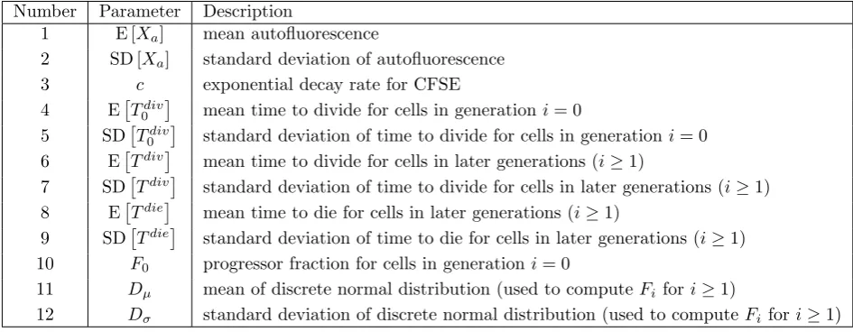
Here, we list the assumptions for the speciﬁc cyton-based mathematical model we consider and describe the parameters that we use to designate this model. All of the parameters for our speciﬁc mathematical model are provided in Table 1.

First, we assume that the random variable Xa is time-independent and has a lognormal distribution with mean and variance denoted E [Xa] and Var [Xa], respectively. Although experiments indicate that the distribution of autofluorescence does, in fact, vary with time, ignoring this time-dependence greatly reduces the number of parameters required to designate the model and still allows for a reasonable fit to summary histogram data [2]. We therefore have two parameters that completely describe the distribution of autofluorescence: E [Xa] and SD [Xa] = (Var [Xa])1/2, which are listed as parameters (1) and (2), respectively, in Table 1.

Next, we assume that the rate of decay in CFSE-induced FI is given by v(t) = c, where c > 0 is some constant. This follows the convention of [2], in which the authors assume that an exponential decay model is suﬃcient to describe decay of CFSE in experiments for whichthe ﬁrst data collection time occurs

after approximately 24 hours. We note that the decay of intracellular CFSE has been observed to occur

(11)

observation can be fully supported with molecular-level modeling [1]. Thus, when data are collected in the ﬁrst 24 hours, it is more accurate to describe the rate of loss of ﬂuorescence intensity with a time-varying rate, as in a Gompertz decay model. For our situation, however, we require only one parameter to completely describe the decay of CFSE:c, which is listed as parameter (3) in the aforementioned table.

We assume that each T_idiv has a lognormal distribution with mean and variance denoted E[T_idiv] and Var[Tdiv

i ]

, respectively. We further assume that, for i ≥ 1, all Tdiv

i are independent and identically dis-tributed (i.i.d.). Such assumptions are consistent with earlier work using the cyton model [2, 12, 13]. We therefore have four parameters that completely describe {Tdiv

i }: E [

Tdiv

0

]

, SD[Tdiv

0

]

= (Var[Tdiv

0

] )1/2_,

E[Tdiv] _{= E}[_Tdiv i

]

for i≥1, and SD[Tdiv] _{= SD}[_Tdiv i

]

= (Var[Tdiv i

]

)1/2 _for_i _≥_{1. These are listed as}

parameters (4) through (7), respectively.

We also assume that the random variables T_idiefori≥1 are i.i.d.with a lognormal distribution, in this case with mean and variance denoted E[Tdie] and Var[Tdie], respectively. Again such assumptions are consistent with earlier work [2, 12, 13]. We further assume that there is no death for undivided cells (i.e., those cells in generation i = 0). In reality, there tends to be a large die-off of cells following stimulation with PHA [6], but we reiterate that for this report the first data were collected approximately 24 hours post-stimulation. As a result,the initial conditions for our mathematical model only reflect those cells that

have not died in the ﬁrst 24 hours after stimulation. Therefore, as in [2], we work under the assumption

that the cells in our “initial population” (consisting of those undivided cells that are still alive 24 hours after stimulation) that do not go on to divide experience essentially no death for the duration of the experiment. Hence, we have two parameters that completely describe {Tdie

i }: E [

Tdie] _{= E}[_Tdie i

]

and SD[Tdie] ₌ SD[Tdie

i ]

= (Var[Tdie i

]

)1/2 _for_i_≥_{1, which are listed as parameters (7) and (8), respectively.}

The only remaining parameters that are required to characterize our model are the progressor fractions {Fi}. We allowF0 to be one of our required model parameters and assume that each progressor fractionFi withi≥1 is uniquely determined by the mean and standard deviation of a “discrete normal distribution”, denoted Dµ and Dσ, respectively. This is consistent with the “division destiny” approach for determining progressor fractions that was employed in [13] and [2], and we refer the interested reader to [2] for a complete discussion of the method by which the progressor fractions are computed. We therefore have three parameters that can be used to determine all the progressor fractions: F0,Dµ, andDσ, which are listed as parameters (10) through (12), respectively.

Thus, our speciﬁc model depends on exactly 12 parameters. We remark that parameters (1) through (3), while important for describing the data, are not considered to be “biologically relevant” parameters in the sense that they do not have any bearing on the proliferative behavior of a population of cells. Also, parameters (4), (6), (8), and (10) are perhaps the most important of the biologically relevant parameters

Number Parameter Description

1 E [Xa] mean autoﬂuorescence

2 SD [Xa] standard deviation of autoﬂuorescence

3 c exponential decay rate for CFSE

4 E[Tdiv

0

]

mean time to divide for cells in generation i= 0

5 SD[T0div

]

standard deviation of time to divide for cells in generation i= 0 6 E[Tdiv] mean time to divide for cells in later generations (i≥1)

7 SD[Tdiv] _{standard deviation of time to divide for cells in later generations (}_i_≥₁₎ 8 E[Tdie] _{mean time to die for cells in later generations (}_i_≥₁₎

9 SD[Tdie] standard deviation of time to die for cells in later generations (i≥1) 10 F0 progressor fraction for cells in generationi= 0

11 Dµ mean of discrete normal distribution (used to computeFi fori≥1)

12 Dσ standard deviation of discrete normal distribution (used to computeFi fori≥1)

(12)

because their interpretation in the context of cell proliferation is the most straightforward. Note that the speciﬁc cyton-based model described here is denoted Model 6 (with exponential label decay) in [2].

4 Parameter Estimation

In order to estimate the parameters in our specific mathematical model, we must first describe a statistical model that relates observable data to the mathematical model. As was previously explained, CFSE flow cytometry data are typically summarized in the form of histograms, and furthermore, measured FI is com-monly represented on a logarithmic scale (cf. Figures 1 through 8). Therefore, we begin by describing how our model can be used to obtain information on cell numbers in a form that can be compared directly with such summarized experimental data.

If we deﬁne the structured densities ˜ni(t,x˜) (in terms ofmeasured FI) as in Section 3, then the structured density for the entire population of cells is

˜

n(t,x˜) = ∞ ∑

i=0

˜

ni(t,x˜)≈ i∑max

i=0

˜

ni(t,x˜).

(See Section 3.1 for a discussion of how to chooseimax appropriately.) Now, because CFSE histogram data are most commonly reported using a base 10 logarithmic scale, we letz= log₁₀(˜x) so that

ˆ

n(t, z) = 10zlog(10) ˜n(t,10z)

gives the structured density in cells per base 10 log unit FI.

In the discussion that follows, we let ⃗q0 denote a hypothetical “true” parameter vector (so that, in the

case of our speciﬁc mathematical model,⃗q0∈R12) and let

I[ˆn](tj, zk;⃗q0) =

∫ zk+1

zk

ˆ

n(tj, z;⃗q0)dz (4.1)

denote the total number of cells with log (base 10) FI in the interval [zk, zk+1] at time tj. Also, we let B denote the (ﬁxed) total number of beads in each sample tube andbj denote the number of beads counted for the sample measured at timetj.

Now, letN_kj be a random variable representing the number of cells with log FI in the interval [zk, zk+1)

measured at timetj. Then it has been argued [2] that

N_kj ∼ N

(

I[ˆn](tj, zk;⃗q0),

B bj

I[ˆn](tj, zk;⃗q0)

)

; (4.2)

i.e., eachN_kj is normally distributed with meanI[ˆn](tj, zk;⃗q0) and variance _bB_jI[ˆn](tj, zk;⃗q0). Note that this

does not lead to either (1) a constant variance model or (2) a constant coeﬃcient of variance model. Though these latter two types of statistical models are commonly assumed to underly data-collection processes [8, 10, 19], modiﬁed residual plots indicate that (4.2) is a better choice in this case [4, 20].

Deﬁne the weighted least squares (WLS) parameter estimator

⃗

qW LS = arg min ⃗

q∈QJ(⃗q;{N j k}),

where

J(⃗q;{N_kj}) =∑ j,k

(I[ˆn](tj, zk;⃗q)−N j k)

2

wj_k ,

Qdenotes the space of allowable parameter vectors, and theweights (selected to match the variance of the

N_kj’s) are given by

wj_k = {_B

bjI[ˆn](tj, zk;⃗q0) forI[ˆn](tj, zk;⃗q0)> I

∗_,

B bjI

∗ _for_I_[ˆ_n_](_t

j, zk;⃗q0)≤I∗.

(13)

The value ofI∗ is positive to prevent division by zero, and in practice it is selected such that the modiﬁed residual plots produce uniform random patterns. We once again follow the convention of [2] and setI∗= 200. If we consider the measured data to be a set of realizations{njk} of the random variables{N_kj}, we can obtain the WLS parameterestimate

ˆ

qW LS = arg min ⃗

q∈QJ(⃗q;{n j

k}). (4.4)

Note that to compute the weights {w_kj} we need ⃗q0, but to estimate ⃗q0 we need the weights. In order to

overcome this obstacle, we use a conventional weighted least squares iterative estimation procedure [8] as described in Algorithm 4.1. In this algorithm, note that ε is a threshold tolerance that allows the user to specify a termination criterion,⃗qtyp is a vector with elements that reﬂect the relative sizes of the parameters to be estimated, and “./” denotes element-wise division.

Algorithm 4.1Parameter Estimation Procedure

1. Obtain initial estimate ˆq(0) _{using (4.4) with}_wj

k = 1 for allj, k.

2. Compute weightswj_k using (4.3) with⃗q0 replaced by ˆq(0).

3. Initialize the iteration counterℓwith the value 1.

4. Do each of the following:

• Compute ˆq(ℓ)_{using (4.4) with current weights} _wj k. • Update the weights using (4.3) with⃗q0 replaced by ˆq(ℓ).

• Store the value of [ˆq(ℓ)−qˆ(ℓ−1)]./[⃗qtyp]in ∆. • Incrementℓby 1.

5. If ∆> ε, return to Step 4. Otherwise, terminate the algorithm.

5 Results and Discussion

In this section, we discuss the results of our study. Since triplicate measurements were collected at each point in a five-day time series, we are able to analyze the variability that exists in the data itself. Also, since these triplicate measurements make it possible to construct a large number of five-day data sets, we are able to analyze variability in the corresponding sets of parameter estimates. We consider experimental variability in the estimates for individual parameters (for each specific combination of donor, ViViD dye status, and cell type) as well as biological variability (i.e., differences between the parameter estimates obtained for different donors and different cell types).

5.1 Variability in the Data

(14)

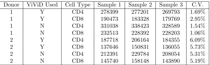
of Figures 1 through 8. Tables 2 through 6 also show an estimate of the coeﬃcient of variation based on each row of sample cell counts. The coeﬃcient of variation is a measure of the relative variation in the cell counts, and can be estimated as

ˆ

cv=

s

¯

x,

where ¯xdenotes the sample mean of the cell counts (in the relevant biological samples) ands denotes the sample standard deviation. We refer to ˆcv as an “estimate” because it is derived from a ﬁnite “sample” of data (in our case, from three cell counts derived from three biological samples). The true coeﬃcient of variation would be computed as

cv =

σ µ,

whereµ andσare the mean and standard deviation, respectively, of cell counts for the “population” of all possible biological samples for the speciﬁc time, donor, ViViD status, and cell type in question.

In order to understand how variation in the cell counts arises, recall from Section 2 that approximately

1 million cells were placed into each of several wells, and that each distinct sample was drawn from a distinct well. Because of the experimental error inherent in seeding the wells, we expect that each well actually started out with a different number of cells. We should remark here that the numbers in Tables 2 through 6 do not represent total cell counts, but rather they represent cell counts for specific types of cells (CD4+ or CD8+ T cells) under specific conditions (donor and ViViD dye status). So, for example, if we attempt to seed 1 million cells from Donor 1 into a well and the true proportion of CD4+ T cells is 15% for this donor, there should be about 150 thousand CD4+ T cells in the well at time t= 0; however, there will be some variation in this number (150 thousand) because of the variation in the total cell population number (1 million). We did not make any measurements at time t= 0, so we cannot directly assess the variation present in the numbers of cells initially seeded into the wells. Our best approximation of this initial variation comes from the cell counts observed on Day 1, which are shown in Table 2. Also, because the true proportion of cells (out of approximately 1 million) corresponding to a particular day, donor, ViViD dye status, and cell type varies, we cannot directly compare all 24 cell count numbers in one of the tables, and we cannot directly compare the 8 sample variances or sample standard deviations obtained for the 8 rows in any given table. To be clear, we cannot use such direct comparisons because themagnitudes of the cell count numbers tend to be different in each row of a given table. We can, however, compare some measure ofrelative variation for each of the rows of a given table. The coefficient of variation described previously is one such measure. So, the 8 numbers listed in the last column of Table 2 give some indication of the variability we expect when attempting to seed 1 million cells into a well, and, importantly, they can be compared with one another.

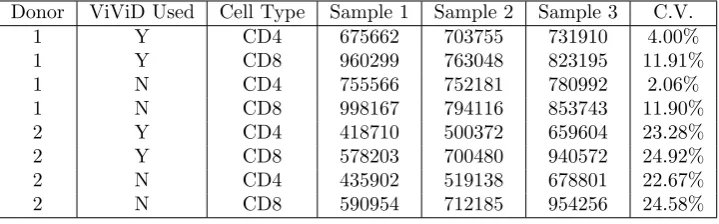
If we assume that the seeding of 1 million cells into a well is a process that is subject to random error, then the amount of error is a random variable with some well-defined probability distribution. For our purposes, the “amount of error in the initial seeding” is synonymous with the “amount of relative variation in the cell counts at Day 1”, which we choose to measure using the coefficients of variation described previously. One important question to consider, then, is whether or not the amount of relative variation in cell counts (or more precisely, the sampling distribution of this statistic) changes between measurement times (days). As was previously asserted, Figures 1 through 8 provide convincing evidence that the amount of relative variation in cell counts does change with respect to time. More specifically, these figures lead us to suspect that there is a significant difference between the relative variation observed in the earlier days of the experiment (1 through 3) and that observed in the later days (4 and 5). The coefficient of variation estimates in the last columns of Tables 2 through 6 can be used to demonstrate this claim conclusively through the use of formal statistical hypothesis testing.

(15)

Donor ViViD Used Cell Type Sample 1 Sample 2 Sample 3 C.V.

1 Y CD4 104124 117820 122408 8.29%

1 Y CD8 36778 38924 40190 4.47%

1 N CD4 128161 140770 146369 6.74%

1 N CD8 39899 42259 43478 4.34%

2 Y CD4 68651 68439 68680 0.19%

2 Y CD8 28699 28574 27387 2.57%

2 N CD4 91542 95914 90740 3.00%

2 N CD8 33983 34605 32692 2.89%

Table 2: Status of cell cultures at Day 1. The numbers in the columns corresponding to Samples 1, 2, and 3 represent cell counts after scaling (using bead counts). Each number in the C.V. column represents the coeﬃcient of variation for the cell counts in the corresponding row.

1 Y CD4 128535 139264 149408 7.51%

1 Y CD8 58115 61406 67116 7.32%

1 N CD4 156211 171078 181924 7.61%

1 N CD8 70147 75010 82658 8.31%

2 Y CD4 66884 63458 63162 3.21%

2 Y CD8 29242 28221 26734 4.49%

2 N CD4 82968 80701 80098 1.86%

2 N CD8 33223 33107 31048 3.77%

1 Y CD4 278399 277201 269793 1.69%

1 Y CD8 190473 183328 179769 2.95%

1 N CD4 331038 338423 328589 1.54%

1 N CD8 232513 228392 228203 1.06%

2 Y CD4 187718 206164 184355 6.09%

2 Y CD8 137646 150831 136055 5.73%

2 N CD4 212391 229784 208054 5.31%

2 N CD8 145740 158148 143890 5.19%

(16)

1 Y CD4 746988 611600 N/A 14.09%

1 Y CD8 778452 616165 N/A 16.46%

1 N CD4 813670 672320 N/A 13.45%

1 N CD8 845757 672287 N/A 16.16%

2 Y CD4 465445 495995 450620 4.92%

2 Y CD8 562295 596485 550758 4.17%

2 N CD4 483623 512917 466908 4.77%

2 N CD8 572560 606627 560635 4.12%

1 Y CD4 675662 703755 731910 4.00%

1 Y CD8 960299 763048 823195 11.91%

1 N CD4 755566 752181 780992 2.06%

1 N CD8 998167 794116 853743 11.90%

2 Y CD4 418710 500372 659604 23.28%

2 Y CD8 578203 700480 940572 24.92%

2 N CD4 435902 519138 678801 22.67%

2 N CD8 590954 712185 954256 24.58%

values (or, equivalently, from two populations with identical cdfs); i.e.,

H0: Fi(x) =Fj(x) for allx.

For the Wilcoxon test, the alternative hypothesis is that one of the two samples was drawn from a population that tends to have larger values than the population from which the other sample was drawn (or, equivalently, that one of the two corresponding distributions isstochastically larger than the other); i.e.,

HA: Fi(x)≤Fj(x) for all x, with strict inequality for at least somex,

or Fi(x)≥Fj(x) for allx, with strict inequality for at least somex.

As with any statistical hypothesis test, the Wilcoxon test produces a “test statistic” that can be converted into a “p-value”. Thep-value indicates the probability of obtaining a test statistic at least as extreme as the one which was actually observedassuming that the null hypothesis is true. If we use a “signiﬁcance level” of 0.05, then we are asserting that outcomes with probability less than 0.05 are unlikely to occur. Therefore, we should reject the null hypothesis whenever thep-value is less than 0.05.

Suppose, for example, that we want to test the claim that there is no diﬀerence between the distribution of relative variations in cell counts observed at Day 1 and that observed at Day 2. This null hypothesis can be formalized as

H0: F1(x) =F2(x) for allx,

(17)

The alternative hypothesis is that one of the two distributions isstochastically larger than the other; i.e.,

HA: F1(x)≤F2(x) for all x, with strict inequality for at least somex,

or F1(x)≥F2(x) for allx, with strict inequality for at least somex.

We can use the coefficient of variation estimates from Tables 2 and 3 to perform a Wilcoxon test for these hypotheses. That is, we can compare the eight coefficient of variation numbers from Table 2 with the eight coefficient of variation numbers from Table 3 using a Wilcoxon test. Based on the p-value of 0.2345 that results from performing this test, we fail to reject the null hypothesis (using a 0.05 significance level) and conclude that there is not a statistically significant difference between the relative variations in cell counts observed at Days 1 and 2, respectively. Similarly, we can perform Wilcoxon tests to conclude that there is not a statistically significant difference between the relative variations in cell counts observed at Days 1 and 3 (p= 0.8785) or the relative variations in cell counts observed at Days 2 and 3 (p= 0.1304). On the other hand, Wilcoxon tests lead us to conclude that thereisa statistically significant difference between the relative variations in cell counts observed at Days 1 and 4 (p= 0.03792) and between the relative variations in cell counts observed at Days 1 and 5 (p= 0.02813). Similarly, there appears to be a statistically significant difference between the relative variations in cell counts observed at Days 2 and 5 (p= 0.03792) and between the relative variations in cell counts observed at Days 3 and 5 (p= 0.01476). (Wilcoxon tests do not indicate a significant difference between relative variations in cell counts observed at Days 2 and 4 or Days 3 and 4, but recall that at least some of the Day 4 coefficients of variation are based on fewer cell counts because fewer biological samples were used for Donor 1 on Day 4; therefore, information concerning variation in cell counts for Day 4 is considerably less reliable.)

We propose that this change in the relative variation of the cell counts with respect to time cannot be explained by proliferation dynamics. In fact, if we assume that our mathematical model describing cell proliferation is correct, the relative variation in cell counts for distinct cultures proliferating with the same dynamics should not change in time. Relative variation can be measured in terms of percent differences or coefficients of variation and we offer proofs of the assertion in the preceding sentence with respect to both of these measures of relative variation in Appendix A of [3], but it is easy (and instructive) to understand the validity of the assertion under the assumption of a simple exponential growth model. So, consider two cultures of cells, “A” and “B”, that are proliferating at the same exponential growth rateα. IfA0 andB0

denote the initial numbers of cells present in cultures A and B, respectively, then

A(t) =A0eαt

and

B(t) =B0eαt

describe the numbers of cells in the respective cultures at time t. The initial percent diﬀerence in the cell counts is

2(A0−B0)

A0+B0

,

while the percent diﬀerence at any later timet is also

2(A0eαt−B0eαt)

A0eαt+B0eαt

=2(A0−B0)e αt

(A0+B0)eαt

=2(A0−B0)

A0+B0

.

Therefore, the percent diﬀerence in cell counts does not change with respect to time. Note that the amount of statistical variation (e.g., diﬀerence) in the cell counts does generally change in time, but the relative

variation (e.g., percent diﬀerence) must remain constant.

(18)

those wells. In fact, the very reason that the nutrient medium is replenished starting at Day 3 is that by

that time it has begun to change color, indicating that the nutrient levels have declined. So, in addition to

the changes in the amount of nutrient available to the cell cultures that occur at discrete points in time corresponding to nutrient medium exchange, we may infer that cells growing and dividing in the various cell cultures signiﬁcantly deplete nutrients in their respective wellsthroughout the experiment.

5.2 Variability in the Parameter Estimates

In order to assess variability in parameter estimates, we applied the parameter estimation technique described in Section 4 to the various five-day time series data sets described in Section 2. For each of the 12 parameters from our specific mathematical model and each of the eight combinations of donor (“Donor1” or “Donor2”), ViViD dye status (“Vivid” indicating that ViViD dye was used to exclude dead cells or “NoVivid” indicating otherwise), and cell type (“CD4” or “CD8”), this led to either 162 or 243 (depending on donor, cf. Section 2) parameter estimates. Each such set of parameter estimates can be represented by a box plot, so for each model parameter we can construct eight box plots. To illustrate this we provide Figure 9, which shows the parameter estimation results for the model parameterscand E[Tdie]for each combination of donor, ViViD dye status, and cell type. The box plots in this figure adhere to the following conventions: (i) the median value is indicated by a red line; (ii) the first and third quartiles (Q1 andQ3) are indicated by the lower and

upper boundaries of the blue box, respectively; (iii) any value that falls aboveQ3+ 1.5(Q3−Q1) or below

Q1−1.5(Q3−Q1) is considered to be an outlier, and is indicated by a “+”; and (iv) the black horizontal lines

above and below the box (which are in most cases connected to the box via dashed vertical lines) represent the maximimum and minimum values, respectively, excluding outliers.

Sets of box plots such as those described above can provide a wealth of information concerning the variability in parameter estimates and identifiability of the corresponding parameters. Individually, each box plot can be used to determine a median parameter estimate and to visualize the variation (spread) in parameter estimates for a given donor and cell type when multiple five-day data sets are considered. The amount of spread in each box plot can also be used to conclude whether or not a particular parameter is likely to be identifiable for any particular donor and cell type. For example, Figure 9 reveals extremely large spreads in many of the box plots corresponding to the parameter E[Tdie], indicating that this model parameter may not be identifiable. On the other hand, all of the box plots corresponding to the parameter

c have relatively small spreads, indicating that this model parameter can be estimated with relatively high reliability.

Taken together, all the box plots corresponding to a given parameter allow for useful comparisons of the parameter estimates that are obtained for different combinations of donor, vivid dye status, and cell type. For example, if we consider the box plots in Figure 9 corresponding to the parameter c, we can make a number of interesting conclusions. First, the use of ViViD dye does not appear to lead to a statistically significant difference in the estimate obtained for the parameter c(cf. box plots 1 and 3, 2 and 4, 5 and 7, and 6 and 8, numbering sequentially from left to right). Next, the estimate forcis larger for CD8+ T cells than for CD4+ T cells when considering data for Donor 1 (cf. box plots 1 and 2 or 3 and 4), but it is larger for CD4+ T cells than for CD8+ T cells when considering data for Donor 2 (cf. box plots 5 and 6 or 7 and 8). Finally, while there does not appear to be a statistically significant difference between Donor 1 and Donor 2 in the estimate obtained forc when considering CD4+ T cells (cf. box plots 1 and 5 or 3 and 7), the Donor 1 estimate is considerably larger than the Donor 2 estimate when considering CD8+ T cells (cf. box plots 2 and 6 or 4 and 8).

5.2.1 Remarks on Basic Parameter Estimates

(19)

3.5 4 4.5 5 5.5 6 6.5 7 7.5 8 8.5

x 10−3

Donor1/Vivid/CD4 Donor1/Vivid/CD8 Donor1/NoVivid/CD4 Donor1/NoVivid/CD8 Donor2/Vivid/CD4 Donor2/Vivid/CD8 Donor2/NoVivid/CD4 Donor2/NoVivid/CD8

Estimates for c

0 50 100 150

Donor1/Vivid/CD4 Donor1/Vivid/CD8 Donor1/NoVivid/CD4 Donor1/NoVivid/CD8 Donor2/Vivid/CD4 Donor2/Vivid/CD8 Donor2/NoVivid/CD4 Donor2/NoVivid/CD8

Estimates for E[Tdie]

(20)

Box plots summarizing estimates for the parameter E [Xa], which represents the mean autofluorescence, are shown in Figure 9 of [3]. The 3rd and 4th box plots in that figure indicate that there is a considerable difference in the mean autofluorescence of CD4+ T cells and CD8+ T cells obtained from Donor 1. (Note that the box plots do not “overlap”.) More specifically, CD8+ T cells appear to have a larger mean auto-fluorescence than CD4+ T cells for Donor 1. On the other hand, the 7th and 8th box plots indicate that CD4+ T cells have a larger mean autofluorescence than CD8+ T cells when considering cells obtained from Donor 2. When we compare CD4+ T cells obtained from the two distinct donors (compare 3rd and 7th box plots), it appears that E [Xa] is larger for Donor 2 than for Donor 1. When comparing CD8+ T cells from the two donors (compare 4th and 8th box plots), it appears that E [Xa] is larger for Donor 1 than for Donor 2.

In Figure 10 of [3], we provide box plots summarizing estimates for standard deviation of the auto-ﬂuorescence, SD [Xa]. As with the mean autoﬂuorescence, it appears that the value of this parameter is larger for CD8+ T cells than for CD4+ T cells in the case of Donor 1 and larger for CD4+ T cells than for CD8+ T cells in the case of Donor 2. Also, when comparing CD4+ T cells obtained from the two distinct donors, it appears that SD [Xa] is larger for Donor 2 than for Donor 1, and when comparing CD8+ T cells from the two donors, it appears that SD [Xa] is larger for Donor 1 than for Donor 2.

Box plots summarizing estimates for the parameter c, which describes exponential decay of CFSE, are shown in Figure 11 of [3]. It appears that the value of this parameter is larger for CD8+ T cells than for CD4+ T cells in the case of Donor 1 and larger for CD4+ T cells than for CD8+ T cells in the case of Donor 2. When we compare CD4+ T cells obtained from the two distinct donors, there does not appear to be a signiﬁcant diﬀerence in the parameterc; however, when comparing CD8+ T cells from the two donors, it appears thatcis larger for Donor 1 than for Donor 2.

In Figure 12 of [3], we provide box plots summarizing estimates for the parameter E[Tdiv

0

] , which represents the mean time to divide for undivided cells. It appears that the value of this parameter is larger for CD4+ T cells than for CD8+ T cells, regardless of which donor we consider. Also, there does not appear to be a signiﬁcant diﬀerence in E[Tdiv

0

]

when comparing CD4+ or CD8+ T cells obtained from the two distinct donors. Figure 13 of [3] indicates that similar statements hold true for SD[T0div

]

, which represents the standard deviation in the time to divide for undivided cells.

Box plots summarizing estimates for the parameter E[Tdiv]_{, which represents the mean time to divide} for cells that have divided at least once, are shown in Figure 14 of [3]. There does not appear to be a signiﬁcant diﬀerence in the value of this parameter for CD4+ and CD8+ T cells, whether we consider cells from Donor 1 or Donor 2. On the other hand, when we compare CD4+ or CD8+ T cells from the two distinct donors, it appears that E[Tdiv] _{is larger for Donor 1 than for Donor 2.}

In Figure 15 of [3], we provide box plots summarizing estimates for the parameter SD[Tdiv], which represents the standard deviation in the time to divide for cells that have divided at least once. For this parameter, there does not appear to be a significant difference in the estimated value when comparing the two cell types from a single donor, or when comparing two donors and a single cell type. Considering the widths of the relevant box plots, we see that there is larger variation in the parameter estimates obtained for CD8+ T cells than those obtained for CD4+ T cells. In fact, the variation in parameter estimates observed for Donor 1 CD8+ T cells is so large as to suggest that this parameter is not identifiable.

Box plots summarizing estimates for the parameter E[Tdie]_{, which represents the mean time to die for} cells that have divided at least once, are shown in Figure 16 of [3]. As was the case with the parameter SD[Tdiv]_{, there does not appear to be a significant difference in the estimated value of the parameter} E[Tdie]_{when comparing the two cell types from a single donor, or when comparing two donors and a single} cell type. For this parameter, we see that there is larger variation in the parameter estimates obtained for Donor 1 cells (of both types) than those obtained for Donor 2 cells. In fact, the variation in parameter estimates observed for Donor 1 cells is so large that it suggests that this parameter is not identifiable.

(21)

the estimates for SD[Tdie]_{obtained for Donor 1 cells (of both types) than those obtained for Donor 2 cells.} The variation in parameter estimates observed for Donor 1 cells is once again so large that it suggests that the parameter SD[Tdie] is also not identiﬁable.

Box plots summarizing estimates for the parameter F0, which represents the progressor fraction for

undivided cells, are shown in Figure 18 of [3]. It appears that the value of this parameter is larger for CD8+ T cells than for CD4+ T cells in the case of Donor 1 and larger for CD4+ T cells than for CD8+ T cells in the case of Donor 2. When we compare CD4+ T cells obtained from the two distinct donors, there does not appear to be a signiﬁcant diﬀerence in the parameterF0; however, when comparing CD8+ T cells from the

two donors, it appears thatF0 is larger for Donor 1 than for Donor 2.

In Figure 19 of [3], we provide box plots summarizing estimates for the parameterDµ. There does not appear to be a significant difference in the value of this parameter for CD4+ and CD8+ T cells in the case of Donor 1, but the parameter value is larger for CD8+ T cells in the case of Donor 2. When we compare CD4+ T cells obtained from the two distinct donors, there does not appear to be a significant difference in the parameterDµ; however, when comparing CD8+ T cells from the two donors, it appears thatDµ is larger for Donor 2 than for Donor 1.

Box plots summarizing estimates for the parameter Dσ are shown in Figure 20 of [3]. It appears that the parameter value is larger for CD8+ T cells than CD4+ T cells in the case of Donor 1, but there does not appear to be a significant difference in the parameter value for CD4+ and CD8+ T cells in the case of Donor 2. When we compare CD4+ T cells obtained from the two distinct donors, it appears that Dσ is larger for Donor 2 than for Donor 1. On the other hand, when comparing CD8+ T cells from the two donors, there does not appear to be a significant difference in the parameterDσ.

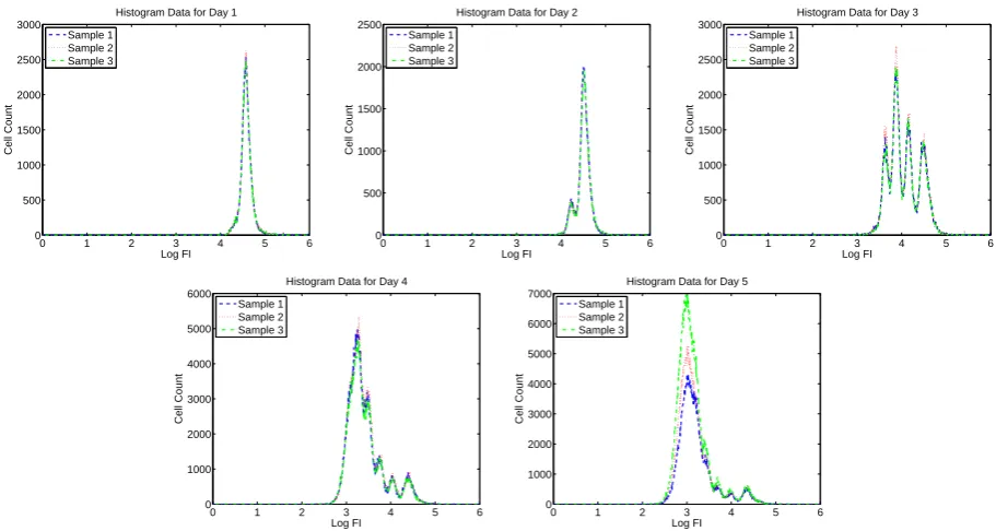
We have already noted that many of our model parameters can be estimated with relatively high re-liability, while others do not appear to be identifiable, but thus far all of our arguments have been based upon visual inspection of the box plots in Figures 9 through 20 of [3]. To allow for more careful quantita-tive analysis of the identifiability of parameters, we provide in Tables 7 through 18 some of the summary statistics used to generate the box plots in those figures. For example, in Table 7 we provide a median and an interquartile range (IQR) corresponding to each of the box plots in Figure 9 of [3]. Since the median and IQR indicate the “center” and “spread”, respectively, for a set of parameter estimates, the ratio of these two quantities provides a useful measure of “relative spread”. We therefore also include a column for the ratio of IQR to median in each of Tables 7 through 18. When the spread is greater than 50% of the central value for a particular set of parameter estimates (i.e., whenever the ratio of IQR to median is greater than 0.50), we consider the variability in that set of parameter estimates to be “relatively high” and conclude that the parameter may not be identifiable; therefore, the ratios meeting this criteria are emphasized in boldface in the tables. Note that the value 0.50 was chosen somewhat arbitrarily, but comparing Tables 7 through 18 with Figures 9 through 20 of [3] makes it clear that such a value for the ratio of IQR to median does, indeed, indicate a “large” relative spread in a set of parameter estimates.

Based on Tables 7 through 18, we conclude that the model parameters E [Xa], SD [Xa], c, E [

Tdiv

0

] , SD[Tdiv

0

]

, E[Tdiv]_,_F

0,Dµ, andDσcan all be estimated with fairly high reliability. On the other hand, the parameters SD[Tdiv]_{, E}[_Tdie]_{, and SD}[_Tdie] _{each have very high ratios of IQR to median in some cases,} indicating that they may not be identifiable. We conjecture that this could be because the mathematical model is not sensitive to these particular parameters. One might reason, for example, that the lack of model sensitivity to the parameters involving “time until death” occurs because divided cells (those cells for which i≥1) tend to divide much more often than they die (when considering stimulated T cells from healthy donors) and such behavior can be correctly incorporated into the model as long as the expected time until division, E[Tdiv]_{, is significantly smaller than the expected time until death, E}[_Tdie]_{. To be} more specific (and to reuse some terminology that was utilized in Section 5.1), as long as the distribution of the random variable Tdie tends to be stochastically larger (by a substantial margin) than that ofTdiv, the correct dynamical behavior of the system can probably be modeled adequately (at least over the first few days) even if the parameters describing the distribution of Tdie are not estimated very accurately. To illustrate this point, consider Figures 10 and 11, in which we plot the (lognormal) distributions of the random variables Tdiv _and _Tdie _{in two different cases. In both cases we use the same set of parameter values for}

(22)

larger than those of Tdiv _{in both cases, so in both situations cells should tend to divide more frequently} than they die. (Recall that the fate of any particular cell is determined by whichever of these two random variables produces a smaller realization.) We argue that, when all other parameters are fixed using some common set of values, the model output does not vary significantly (at least over the first few days) when the two different sets of parameter values forTdieindicated in Figures 10 and 11 are used. To demonstrate this claim, we show sample model output generated using these two different sets of parameter values forTdie in Figure 12. The complete sets of parameter values for “Model A” and “Model B” are provided in Table 19. Note that, despite the large discrepancy in the values used for E[Tdie] _{and SD}[_Tdie]_{, the output for the} two models is indistinguishable until at least Day 4. This simple exercise indicates that the accuracy of data collected in the later days of the experiment may be critical to the correct identification of the parameters E[Tdie]_{and SD}[_Tdie]_.

5.2.2 Parameter Estimates Obtained Using Fixed Values for Some Parameters

By examining scatter plots of various pairings of parameter estimates, we can determine whether or not any correlations might exist between some of the parameters. For example, Figures 13 and 14 indicate a strong

Donor ViViD Used Cell Type Median IQR IQR/Median

1 Y CD4 402.30 32.58 0.0810

1 Y CD8 680.44 79.29 0.1165

1 N CD4 388.45 25.33 0.0652

1 N CD8 678.97 81.78 0.1204

2 Y CD4 623.98 50.55 0.0810

2 Y CD8 542.52 21.49 0.0396

2 N CD4 630.26 82.19 0.1304

2 N CD8 536.94 24.43 0.0455

Table 7: Summary statistics for estimates of parameter E [Xa] (cf. Figure 9 of [3]).

1 Y CD4 227.87 17.03 0.0747

1 Y CD8 339.49 78.22 0.2304