R E S E A R C H
Open Access
Cooperative localization by dual foot-mounted
inertial sensors and inter-agent ranging
John-Olof Nilsson
*, Dave Zachariah, Isaac Skog and Peter Händel
Abstract
The implementation challenges of cooperative localization by dual foot-mounted inertial sensors and inter-agent ranging are discussed, and work on the subject is reviewed. System architecture and sensor fusion are identified as key challenges. A partially decentralized system architecture based on step-wise inertial navigation and step-wise dead reckoning is presented. This architecture is argued to reduce the computational cost and required
communication bandwidth by around two orders of magnitude while only giving negligible information loss in comparison with a naive centralized implementation. This makes a joint global state estimation feasible for up to a platoon-sized group of agents. Furthermore, robust and low-cost sensor fusion for the considered setup, based on state space transformation and marginalization, is presented. The transformation and marginalization are used to give the necessary flexibility for presented sampling-based updates for the inter-agent ranging and ranging free fusion of the two feet of an individual agent. Finally, the characteristics of the suggested implementation are demonstrated with simulations and a real-time system implementation.
Keywords: Cooperative localization; Pedestrian localization; Pedestrian dead reckoning; Inertial navigation; Infrastructure-free localization
1 Introduction
High accuracy, robust, and infrastructure-free pedestrian localization is a highly desired ability for, among oth-ers, military, security personnel, and first responders. Localization and communication are key capabilities to achieve situational awareness and to support, manage, and automatize individual’s or agent group actions and interactions. See [1-8] for reviews on the subject. The fundamental information sources for the localization are proprioception, exteroception, and motion models. With-out infrastructure, the exteroception must be dependent on prior or acquired knowledge about the environment [9]. Unfortunately, in general, little or no prior knowledge of the environment is available, and exploiting acquired knowledge without revisiting locations is difficult. There-fore, preferably the localization should primarily rely on proprioception and motion models. Proprioception can take place on the agent level, providing the possibil-ity to perform dead reckoning, or on inter-agent level,
*Correspondence: [email protected]
Signal Processing Department, ACCESS Linnaeus Centre, KTH Royal Institute of Technology, Osquldas väg 10, SE-100 44 Stockholm, Sweden
providing the means to perform cooperative localiza-tion. Pedestrian dead reckoning can be implemented in a number of different ways [10]. However, foot-mounted inertial navigation, with motion models providing zero-velocity updates, constitute a unique, robust, and high-accuracy pedestrian dead reckoning capability [11-14]. With open-source implementations [15-17] and several products appearing on the market [18-21], dead reckon-ing by foot-mounted inertial sensors is a readily avail-able technology. In turn, the most straightforward and well-studied inter-agent measurement, and mean of coop-erative localization, is ranging [22-25]. Also here, there are multiple (radio) ranging implementations available in the research literature [26-30] and as products on the market [31-33]. Finally, suitable infrastructure-free com-munication equipment for inter-agent comcom-munication is available off-the-shelf, e.g. [34-37], and processing plat-forms are available in abundance. Together, this suggests that the setup with foot-mounted inertial sensors and inter-agent ranging as illustrated in Figure 1 is suitably used as a base setup for any infrastructure-free pedestrian localization system. However, despite the mature compo-nents and the in principle straight-forward combination,
Dual foot-mounted inertial sensors Inter-agent
ranging
Inter-agent com. Com. and
proc. device
Ranging device
Local com. Local
com.
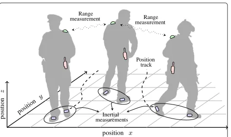
Figure 1Illustration of the considered localization setup.A group of agents are cooperatively localizing themselves without any infrastructure. For this purpose, each agent is equipped with dual foot-mounted inertial sensors, a ranging device, and a communication (com.) and processing (proc.) device.
cooperative localization with this sensor setup remains challenging, and only a few similar systems can be found in the literature [38-42], and no off-the-shelf products are available.
The challenges with the localization setup lie in the sys-tem architecture and the sensor fusion. The inter-agent ranging and lack of anchor nodes mean that some global state estimation is required with a potentially prohibitive large computational cost. The global state estimation, the distributed measurements, and the (required) high sam-pling rates of the inertial sensors mean that a potentially substantial communication is needed and that the system may be sensitive to incomplete or varying connectiv-ity. The feet are poor placements for inter-agent ranging devices and preferably inertial sensors are used on both feet, meaning that the sensors of an individual agent will not be collocated. This gives a high system state dimen-sionality and means that relating the sensory data from different sensors to each other is difficult and that local communication links on each agent are needed. Further, inter-agent ranging errors as well as sensor separations, often have far from white, stationary, and Gaussian char-acteristics. Together, this makes fusing ranging and dead reckoning in a high integrity and recursive Bayesian man-ner at a reasonable computational cost difficult.
Unfortunately, the mentioned challenges are inherent to the system setup. Therefore, they have to be addressed for any practical implementation. However, to our knowl-edge, the implementation issues have only been sparsely covered in isolation in the literature, and no complete sat-isfactory solution has been presented. Therefore, in this article, we present solutions to key challenges to the sys-tem setup and a complete localization syssys-tem implemen-tation. More specifically, the considered overall problem is tracking, i.e., recursively estimating, the positions of a
group of agents with the equipment setup of Figure 1. The available measurements for the tracking are iner-tial measurements from the dual foot-mounted ineriner-tial sensors and inter-agent range measurements. The posi-tion tracking is illustrated in Figure 2. The measurements will be treated as localized to the respective sensors, and the necessary communication will be handled as an inte-gral part of the overall problem. However, we will not consider specific communication technologies but only communication constraints that naturally arise in the cur-rent scenario (low bandwidth and varying connectivity). See [43-47] and references therein for treatment of related networking and communication technologies. Also, for brevity, the issues of initialization and time synchroniza-tion will not be considered. See [48,49] for the solusynchroniza-tions used in the system implementation.
position position
p
o
sition
Position track Range
measurement Range measurement
Inertial measurements
To arrive at the key challenges and the solutions, initially, in Section 2, the implementation challenges are discussed in more detail, and the related work is reviewed. Following this, we address the key challenges and present a cooperative localization system implemen-tation based on dual foot-mounted inertial sensors and inter-agent ranging. The implementation is based on a partially decentralized system architecture and statisti-cal marginalization, and sampling-based measurement updates. In Section 3, the architecture is presented and argued to reduce the computational cost and required communication by around two orders of magnitude, and to make the system robust to varying connectivity, while only giving negligible information loss. Thereafter, in Section 4, the sampling-based measurement updates with required state space transformation and marginalization are presented and shown to give a robust and low com-putational cost sensor fusion. Subsequently, in Section 5, the characteristic of the suggested implementation is illustrated via simulations and a real-time system imple-mentation. The cooperative localization is found to give a bounded relative position mean square error (MSE) and an absolute position MSE inversely proportional to the number of agents, in the worst case scenario, and a bounded position MSE in the best case scenario. Finally, Section 6 concludes the article.
2 Implementation challenges
The lack of anchor nodes, the distributed nature of the system, the error characteristics of the different sensors, and the non-collocated sensors of individual agents poses a number of implementation challenges for the coop-erative localization. Broadly speaking, these challenges can be divided into those related to designing an overall system architecture to minimize the required communi-cation and computational cost, while making it robust to varying connectivity and retaining sufficient information about the coupling of non-collocated parts of the sys-tem, and fusing the information of different parts of the system given the constraints imposed by the system archi-tecture and a finite computational power, while retaining performance and a high system integrity. In the following two subsections, these two overall challenges are dis-cussed in more detail, and the related previous work is reviewed.
2.1 System architecture and state estimation
The system architecture has a strong connection to the position/state estimation and the required communica-tion. The range of potential system architectures and estimation solutions goes from the completely decentral-ized, in which each agent only estimates its own states, to the completely centralized, in which all states of all agents are estimated jointly.
A completely decentralized architecture is often used in combination with some inherently decentralized belief propagation estimation techniques [38,50,51]. The advan-tage of this is that it makes the localization scalable and robust to varying and incomplete connectivity between the agents. Unfortunately, belief propagation discards information about the coupling between agents, lead-ing to reduced performance [51-54]. See [52] for an explicit treatment of the subject. Unfortunately, as will be shown in Section 5, in a system with dead reckon-ing, inter-agent rangreckon-ing, and no anchor nodes, the errors in the position estimates of the different agents may become almost perfectly correlated. Consequently, dis-carding these couplings/correlations between agents can significantly deteriorate the localization performance and integrity.
In contrast, with a centralized architecture and esti-mation, all correlations can be considered, but instead the state dimensionality of all the agents will add up. Unfortunately, due to the lack of collocation of the sen-sors of the individual agents, the state dimensionality of the individual agents will be high. Together, this means computationally expensive filter updates. Further, the distributed nature of the system means that informa-tion needs to be gathered to perform the sensor fusion. Therefore, communication links are needed, both locally on each agent as well as on a group level. Inter-agent communication links are naturally wireless. However, the foot-mounting of the inertial sensors makes cabled connections impractical, opting for battery powering and local wireless links for the sensors as well [55,56]. Unfor-tunately, the expensive filter updates, the wireless com-munication links, and the battery powering combines poorly with the required high sampling rates of the inertial sensors. With increasing number of agents, the compu-tational cost and the required communication bandwidth will eventually become a problem. Moreover, an agent which loses contact with the fusion center cannot, unless state statistics are continually provided, easily carry on the estimation of its own states by itself. Also, to recover from an outage when the contact is restored, a significant amount of data would have to be stored, transferred, and processed.
or required guaranteed and high bandwidth communi-cation, and are not adapted to the considered sensor setup with high update rates, local communication links, and lack of sensor collocation. Therefore, in Section 3, we suggest and motivate a system architecture with par-tially decentralized estimation based on a division of the foot-mounted inertial navigation into a step-wise inertial navigation and dead reckoning. This architec-ture does not completely solve the computational cost issue but makes it manageable for up to a platoon-sized group of agents. For larger groups, some cellular structure is needed [39,58]. However, the architecture is largely independent of how the global state estima-tion is implemented and a distributed implementaestima-tion is conceivable.
The idea of dividing the filtering is not completely new. A similar division is presented in an application specific context in [60] and used to fuse data from foot-mounted inertial sensors with maps, or to build the maps themselves, in [61-63]. However, the described divi-sion is heuristically motivated, and the statistical relation between the different parts is not clear. Also, no physical processing decentralization is exploited to give reduced communication requirements.
2.2 Robust and low computational cost sensor fusion
The sensor fusion firstly poses the problem of how to model the relation between the tracked inertial sensors and the range measurements. Secondly, it poses the prob-lem of how to condition the state statistic estimates on provided information while retaining reasonable compu-tational costs.
The easiest solution to the non-collocated sensors of individual agents is to make the assumption that they are collocated (or have a fixed relation) [38,64-66]. While simple, this method can clearly introduce mod-eling errors, resulting in suboptimal performance and questionable integrity. Instead, explicitly modeling the relative motion of the feet has been suggested in [67]. However, making an accurate and general model of the human motion is difficult, to say the least. As an alter-native, multiple publications suggest explicitly measur-ing the relation between the sensors [14,68-70]. The added information can improve the localization perfor-mance but unfortunately introduces the need for addi-tional hardware and measurement models. Also, it works best for situations with line-of-sight between measure-ment points, and therefore, it is probably only a viable solution for foot-to-foot ranging on clear, not too rough, and vegetation/obstacle-free ground [71]. Instead of mod-eling or measuring the relation between navigation points of an individual agent, the constraint that the spatial sep-aration between them has an upper limit may be used. This side information obviously has an almost perfect
integrity, and results in [72] indicate that the perfor-mance loss in comparison to ranging is transitory. For inertial navigation, it has been demonstrated that a range constraint can be used to fuse the information from two foot-mounted systems, while only propagating the mean and the covariance [73,74]. Unfortunately, the sug-gested methods depend on numerical solvers and only apply the constraint on the mean, giving questionable statistical properties. Therefore, in Section 4, based on the work in [72], we suggest a simpler and numerically more attractive solution to using range constraints to per-form the sensor fusion, based on marginalization and sampling.
The naive solution to the sensor fusion of the foot-mounted inertial navigation and the inter-agent ranging is simply using traditional Kalman filter measurement updates for the ranging [38]. However, the radio rang-ing errors are often far from Gaussian, often with heavy tails and non-stationary and spatially correlated errors [75-80]. This can cause unexpected behavior of many localization algorithms, and therefore, statistically more robust methods are desirable [79-81]. See [82] and ref-erences therein for a general treatment of the statistical robustness concept. The heavy tails and spatially corre-lated errors could potentially be solved by a flat likelihood function as suggested in [75,83]. However, while giving a high integrity, this also ignores a substantial amount of information and requires multi-hypothesis filtering (a particle filter) with unacceptable high computational cost. Using a more informative likelihood function is not hard to imagine. Unfortunately, only a small set of like-lihood functions can easily be used without resorting to multi-hypothesis filtering methods. Some low-cost fusion techniques for special classes of heavy-tailed distributions and H∞ criteria have been suggested in the literature [84-88]. However, ideally, we would like more flexibility to handle measurement errors and non-collocated sensors. Therefore, in Section 4, we propose a marginalization and sample based measurement update for the inter-agent ranging, providing the necessary flexibility to handle an arbitrary likelihood function. A suitable likelihood func-tion is proposed, taking lack of collocafunc-tion, statistical robustness, and correlated errors into account, and shows to provide a robust and low computational cost sensor fusion.
3 Decentralized estimation architecture
with computational cost, communication bandwidth, and robustness to varying connectivity. In the following sub-sections, it is shown how this can be achieved by dividing the filtering associated with foot-mounted inertial sen-sors into a step-wise inertial navigation and step-wise dead reckoning. Pseudo-code for the related processing is found in Algorithm 1.
3.1 Zero-velocity-update-aided inertial navigation
To track the position of an agent equipped with foot-mounted inertial sensors, the sensors are used to imple-ment an inertial navigation system aided by so called zero-velocity updates (ZUPTs). The inertial navigation essentially consists of the inertial sensors combined with mechanization equations. In the simplest form, the mech-anization equations are
wherekis a time index,dtis the time difference between measurement instances,pkis the position,vkis the veloc-ity,fk is the specific force,g =[0, 0,g] is the gravity, and
ωkis the angular rate (all inR3). Further,qkis the quater-nion describing the orientation of the system, the triple productqk−1fkqk−1denotes the rotation offk byqk, and
(·)is the quaternion update matrix. For a detailed treat-ment of the inertial navigation, see [89,90]. For analytical convenience, we will interchangeably represent the orien-tationqkwith the equivalent Euler angles (roll, pitch, yaw)
θk =[φk,θk,ψk]. Note that [·,. . .] is used to denote a column vector.
The mechanization equations (1) together with mea-surements of the specific force ˜fk and the angular rates
˜
ωk, provided by the inertial sensors, are used to propagate positionpˆk, velocityvˆk, and orientationqˆkstate estimates. Unfortunately, due to its integrative nature, small mea-surement errors in˜fk andω˜k accumulate, giving rapidly growing estimation errors. Fortunately, these errors can be modeled and estimated with ZUPTs. A first-order error model of (1) is given by and zero matrices, respectively, and [·]× is the cross-product matrix. As argued in [91], one should be cautious about estimating systematic sensor errors in the current setup. Indeed, remarkable dead reckoning performance has been demonstrated, exploiting dual foot-mounted sensors without any sensor error state estimation [92].
Therefore, in contrast to many publications, no additional sensor bias states are used.
Together with statistical models for the errors in˜fkand ˜
ωk, (2) is used to propagate statistics of the error states. To estimate the error states, stationary time instances are detected based on the condition Z({˜fκ,ω˜κ}Wk) < γZ,
whereZ(·)is some zero-velocity test statistic,{˜fκ,ω˜κ}Wk
is the inertial measurements over some time windowWk, andγZis a zero-velocity detection threshold. See [93,94]
for further details. The implied zero-velocities are used as pseudo-measurements
˜
yk = ˆvk∀k:Z({˜fκ,ω˜κ}Wk) < γZ, (3)
which are modeled in terms of the error states as
˜ is also used to lock the system when completely stationary. See [95] for further details. Given the error model (2) and the measurements model (4), the measurements (3) can be used to estimate the error states with a Kalman type of filter. See [11,94,96,97] for further details and variations. See [98] for a general treatment of aided navigation. Since there is no reason to propagate errors, as soon as there are any non-zero estimatesδpˆk,δvˆk, orδθˆk, they are fed back and consequently, the error state estimates are set to zero, i.e.,δpˆk := 03×1,δvˆk :=03×1, andδθˆk :=03×1, where :=
indicates assignment.
Unfortunately, all (error) states are not observable based on the ZUPTs. During periods of consecutive ZUPTs, the system (2) becomes essentially linear and time invariant. Zero-velocity for consecutive time instances means no acceleration and ideallyfk =qkgqk. This gives the system
the roll and pitch are observable, while the heading (yaw) of the system is not. Ignoring the process noise, this implies that the covariances of the observable states decay as one over the number of consecutive ZUPTs. Note that there is no difference between the covariances of the error states and the states themselves. Consequently, during standstill, after a reasonable number of ZUPTs, the state estimate covariance becomes
cov(pˆk,vˆk,θˆk)
≈ ⎡
⎣0P5p×k3 0053××55 P0p5k×,ψ1k Pp
k,ψk 01×5 Pψk,ψk,
⎤
⎦ (6)
wherePx,y=cov(x,y),Px=cov(x)=cov(x,x),(·)denotes the transpose, and 0n×m denotes a zero matrix of size
n×m.
3.2 Step-wise dead reckoning
The covariance matrix (6) tells us that the errors of pˆk and ψˆk are uncorrelated with those of vˆk and [φˆk,θˆk]. Together with the Markovian assumption of the state space models and the translational and in-plan rotation invariance of (1) to (4), this means that future errors of
ˆ
vk and [φˆk,θˆk] are uncorrelated with those of the current ˆ
pk andψˆk. Consequently, future ZUPTs cannot be used to deduce information about the current position and heading errors. In turn, this means that, considering only the ZUPTs, it makes no difference if we reset the system and add the new relative position and heading to those before the reset. However, for other information sources, we must keep track of the global (total) error covariance of the position and heading estimates.
Resetting the system means setting position pˆk and heading ψˆk, and corresponding covariances to zero. Denote the position and heading estimates at a reset
by dp and dψ. These values can be used to drive the
step-wise dead reckoning
x
χ
=
x−1
χ−1
+
R−1dp
dψ
+w, (7)
wherex andχ are the global position in three
dimen-sions and heading in the horizontal plan of the inertial navigation system relative to the navigation frame,
R= ⎡
⎣cossin(χ(χ)) −cossin(χ(χ)) 00
0 0 1
⎤ ⎦
is the rotation matrix from the local coordinate frame of the last reset to the navigation frame, and w is a (by
assumption) white noise with covariance,
cov(w)=cov([R−1dp,dψ]) =
R−1PpR−1 R−1Pp,ψ Pp
,ψR
−1 Pψ,ψ
. (8)
The noise w in (7) represents the accumulated
uncer-tainty in position and heading since the last reset, i.e., the essentially non-zero elements in (6) transformed to the navigation frame. The dead reckoning (7) can trivially be used to estimatex and χ, and their error covariances
from dp and dψ, and related covariances. The
rela-tion between the step-wise inertial navigarela-tion and dead reckoning is illustrated in Figure 3.
To get [dp,dψ] from the inertial navigation, reset
instances need to be determined, i.e., the decoupled sit-uation (6) needs to be detected. However, detecting it is not enough. If it holds for one time instancek, it is likely to hold for the next time instance. Resetting at nearby time instances is not desirable. Instead we want to reset once at every step or at some regular intervals if the sys-tem is stationary for a longer period of time. The latter requirement is necessary to distinguish between extended stationary periods and extended dynamic periods. Fur-ther, to allow for real-time processing, the detection needs to be done in a recursive manner. The longer the sta-tionary period, the smaller the cross-coupling terms in (6). This means that the system should be reset as late as possible in a stationary period. However, if the sta-tionary period is too short, we may not want to reset at all, since then the cross-terms in (6) may not have converged.
In summary, thenecessary conditionsfor a reset are low enough cross-coupling and minimum elapsed time since the last reset. If this holds, there is a pending reset. In principle, the cross-coupling terms in (6) should be used to determine the first requirement. However, in practice, all elements fall off together, and a thresholdγpon, e.g., the first velocity component, can be used. To assess the second requirement, a countercp which is incremented at each time instance is needed, giving the pending reset condition
(Pvxk < γp)∧(cp>cmin), (9)
wherecminis the minimum number of samples between
resets. A pending reset is to be performed if the stationary period comes to an end or a maximum time with a pend-ing reset has elapsed. To assess the latter condition, a counter cd is needed which is incremented if (9) holds. Then, a reset is performed if
Z({˜fκ,ω˜κ}Wk)≥γZ
∨(cd>cmax), (10)
wherecmaxis the maximum number of samples of a
pend-ing reset. Together, (9) and (10) make up the sufficient conditionsfor a reset. When the reset is performed, the counters are reset, cp := 0 and cd := 0. This gives a recursive step segmentation. Pseudo-code for the inertial navigation with recursive step segmentation (i.e., step-wise inertial navigation) and the step-step-wise dead reckoning is found in Algorithm 1.
Algorithm 1 Pseudo-code of the combined step-wise inertial navigation and step-wise dead reckoning. The ZUPT-aided inertial navigation and the step-wise dead reckoning refer to the effect of (1) to (5) and (7), respec-tively, combined with Kalman type of filtering. For nota-tional compactness, below Pk = P[pk,vk,qk] and P =
P[x,χ].
1: k:=:=cp:=cd :=0 2: pk :=vk :=03×1
3: qk := {Coarse self-initialization}(see, e.g., [98]) 4: Pk := {Initial velocity, roll, and pitch uncertainty} 5: (x,χ):= {Initial position and heading}
6: P(x,χ):= {Initial position and heading uncertainty}
7: loop 8: k:=k+1
9: ZUPT-aided inertial navigation
([pk,vk,qk] ,Pk)←([pk−1,vk−1,qk−1] ,Pk−1,˜fk,ω˜k) 10: cp:=cp+1
11: if(Pvk < γp)∧(cp>cmin)then
12: cd:=cd−1+1
13: if
Z({˜fκ,ω˜κ}Wk)≥γZ
∨(cd>cmax)then
14: :=+1
15: dp:= ˆpk, dψ:= ˆφk, Pw =. . . (see (8))
16: pk:=vk :=03×1, ψk:=0 17: Pk:=09×9
18: cp:=0, cd :=0
19: Step-wise dead reckoning
([x,χ] ,P) ←
([x−1,χ−1] ,P−1,dp,dψ,Pw)
20: end if
21: end if 22: end loop
Not to lose performance in comparison with a sen-sor fusion approach based on centralized estimation, the wise inertial navigation combined with the step-wise dead reckoning needs to reproduce the same state statistics (mean and covariance) as those of the indef-inite (no resets) ZUPT-aided inertial navigation. If the models (1), (2), and (7) had been linear with Gaussian noise and the cross-coupling terms of (6) were perfectly zero, then the divided filtering would reproduce the full filter behavior perfectly. Unfortunately, they are not. How-ever, as shown in the example trajectory in Figure 4, in practice, the differences are marginal, and the mean and covariance estimates of the position and heading can be reproduced by only [dp,dψ] and the
correspond-ing covariances. Due to linearization and modelcorrespond-ing errors of the ZUPTs, the step-wise dead reckoning can even be expected to improve performance since it will elim-inate these effects to single steps [91,99]. Indeed, reset-ting appropriate covariance elements (which has similar effects as of performing the step-wise dead reckoning) has empirically been found to improve performance [100].
3.3 Physical decentralization of state estimation
The step-wise inertial navigation and dead reckoning as described in Algorithm 1 can be used to implement a
decentralized architecture and state estimation. The rang-ing, as well as most additional information, is only depen-dent on position, not on the full state vector [pk,vk,θk]. Further, as argued in the previous subsection, the errors ofvkˆ and [φˆk,θˆk] are weakly correlated with those ofpkˆ and ψˆk. Therefore, only the states [x,χ] (for all feet)
have to be estimated jointly, and only line 19 needs to be executed centrally. The step-wise inertial navigation, i.e., Algorithm 1 apart from line 19, can be implemented locally in the foot-mounted units, and thereby, only [dp,dψ] and related covariances need to be
transmit-ted from the feet. This way, the required communication will be significantly lower compared to that in the case in which all inertial data would have to be transmitted. Also, since the computational cost of propagating (7) is marginal, this can be done both locally on the process-ing device of each agent and in a global state estimation. This way, if an agent loses contact with whomever who performs the global state estimation, it can still perform the dead reckoning and, thereby, keep an estimate of where it is. Since the amount of data in the displacement and heading changes is small, if contact is reestablished, all data can easily be transferred, and its states in the global state estimation updated. The other way around, if corrections to the estimates of [x,χ] are made in the
central state estimation, these corrections can be trans-ferred down to the agent. Since the recursion in (7) is pure dead reckoning (no statistical conditioning), these correc-tions can directly be used to correct the local estimates of [x,χ]. This way, the local and the global estimates can
be kept consistent.
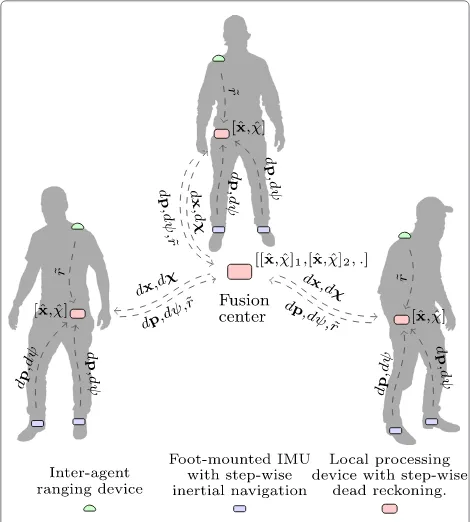
The straightforward way of implementing the global state estimation is by one (or multiple) central fusion center to which all dead reckoning data are transmitted (potentially by broadcasting). The fusion center may be carried by an agent or reside in a vehicle or something similar. Range measurements relative to other agents only have a meaning if the position estimate and its statis-tics are known. Therefore, all ranging information is transferred to the central fusion center. This process-ing architecture with its three layers of estimation (foot, processing device of agent, and common fusion cen-ter) is illustrated in Figure 5. However, the division in step-wise inertial navigation and dead reckoning is inde-pendent of the structure with a fusion center, and some decentralized global state estimation could potentially be used.
3.4 Computational cost and required communication
The step-wise dead reckoning is primarily motivated and justified by the reduction in computational cost and required communication bandwidth. With a completely centralized sensor fusion [˜fk,ω˜k], six measurement val-ues in total, needs to be transferred to the central fusion
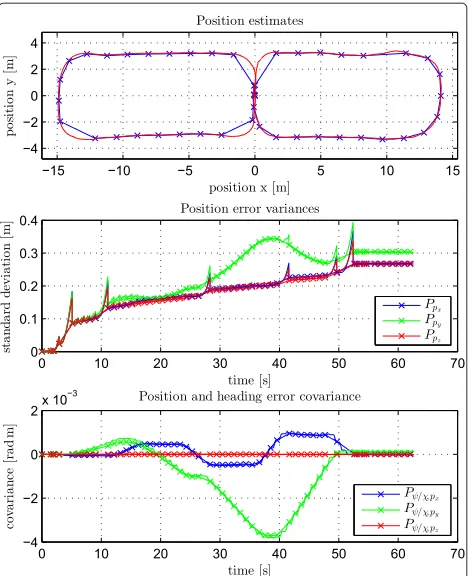
Figure 5Comparison of step-wise dead reckoning and indefinite ZUPT-aided inertial navigation.The plots show the trajectory (top), the position error covariances (middle), and the covariance between the position and heading errors (bottom) as estimated by an extended Kalman filter-based indefinite ZUPT-aided inertial navigation (solid lines) and a step-wise inertial navigation and dead reckoning (crossed lines). The agreement between the systems is far below the accuracy and integrity of the former system.
center at a sampling ratefIMU in the order of hundreds
of Hz, with each measurement value typically consisting of some 12 to 16 bits. With the step-wise dead reckon-ing, [dp,dψ],Pp,Pp,ψ, andPψ,ψ, in total 14 values, need to be transferred to the central fusion center at a rate offsw≈1 Hz (normal gait frequency [101]). In
prac-tice, the 14 values can be reduced to 8 values since cross-covariances may be ignored, and the numerical ranges are such that they can reasonably be fitted in some 12 to 16 bits each. The other way around, some four cor-rection values need to be transferred back to the agent. Together, this gives the ratio of the required communica-tion of(6·fIMU)/(12·fsw)≈102, a two-order magnitude
reduction. In turn, the computational cost scales linearly with the update ratesfIMUandfsw. In addition, the
practice, giving a reduction of again around two orders of magnitude.
4 Robust and low-cost sensor fusion
The step-wise dead reckoning provides a low-dimensional and low-update rate interface to the foot-mounted iner-tial navigation. With this interface, the global state of the localization system (the system state as conceived by the global state estimation) becomes
x=[xα,χα,xβ,χβ,xζ,χζ,. . .],
where xj and χj are the positions and headings of the agents’ feet with dropped time indices. Other auxiliary states may also be put in the state vector. Our desire is to fuse the provided dead reckoning with that of the other foot and that of the other agents via inter-agent ranging. This fusion is primarily challenging because of (1) the high dimensionality of the global system, (2) the non-collocated sensors of individual agents, and (3) the potentially malign error characteristic of the ranging. The high dimensionality is tackled by only propagating the mean and covariance estimates and by marginal-ization of the state space. The lack of collocation is handled by imposing range constraints between sensors. Finally, the error characteristic of the ranging is handled by sampling-based updates. In the following subsections, these approaches are described. The pseudo-code for the sensor fusion is found in Algorithms 2 and 3 in the final subsection.
4.1 Marginalization
New information (e.g., range measurements) introduced in the systems is only dependent on a small subset of the states. Assume that the state vector can be decomposed asz =[z1,z2], such that some introduced informationπ
is only dependent onz1. Then, with a Gaussian prior with
mean and covariance,
ˆ z=
ˆ z1 ˆ z2
and Pz=
Pz1 Pz1z2
Pz1z2 Pz2, , (11)
the conditional (with respect to π) mean of z2 and the
conditional covariance can be expressed as [72]
ˆ
z2|π= V+Uzˆ1|π
Pz1|π= Cz1|π− ˆz1|πzˆ1|π
Pz2|π= Pz2−UPz1z2+VV+Z+UCz1|πU−ˆz2|πzˆ2|π
Pz1z2|π= ˆz1|πV+Cz1|πU− ˆz1|πzˆ2|π,
(12)
whereU = Pz1z2P−z11,V = ˆz2−Uzˆ1,Z = Uzˆ1|πV+ Vzˆ1|πU, and Cz1|π is the conditional second order
moment ofz1. Note that this will hold for any information
πonly dependent onz1, not just range constraints as
stud-ied in [72]. Consequently, the relations (12) give a desired marginalization. To impose the information π on (11), only the first and second conditional moments,zˆ1|π and Cz1|π, need to be calculated. Ifπis linearly dependent on z1and with Gaussian errors, this will be equivalent with
a Kalman filter measurement update. This may trivially be used to introduce information about individual agents. However, as we will show in the following subsections, this can also be used to couple multiple navigation points of individual agents without any further measurement and to introduce non-Gaussian ranging between agents.
4.2 Fusing dead reckoning from dual foot-mounted units
The position of the feetxaandxbof an agent (in general two navigation points of an agent) has a bounded spatial separation. This can be used to fuse the related dead reck-oning without any further measurements. In practice, the constraint will often have different extents in the vertical and the horizontal directions. This can be expressed as a range constraint
Dγ(xa−xb) ≤γxy, (13)
whereDγis a diagonal scaling matrix withγ=[1,1,γxy/γz] on the diagonal, and γxy and γz are the constraints in the horizontal and vertical direction. Unfortunately, there is no standard way of imposing such a constraint in a Kalman-like framework [102]. Also, the position states being in arbitrary locations in the global state vector, i.e., x=[. . .,xa,. . .,xb,. . .], means that the state vector is not on the form ofz. Further, since the constraint (13) has unbounded support, the conditional means xˆa|γ,xˆb|γ
and covariances cov[xa|γ,xb|γ]
cannot easily be eval-uated. Moreover, since the states are updated asyn-chronously (steps occurring at different time instances), the state estimatesxaˆ andxˆb may not refer to the same time instance. The latter problem can be handled by adjusting the constraintγxy by the time difference of the states. In principle, this means that an upper limit on the speed by which an agent moves is imposed. The former problems can be solved with the state transformation
z=Tγx where Tγ =
Dγ −Dγ
Dγ Dγ
⊕Im−6
, (14)
whereIm−6is the identity matrix of sizem−6,mis the
dimension ofx,⊕denotes the direct sum of matrices,
is a permutation matrix fulfilling
andz1=Dγ(xa−xb). With the state transformationTγ,
the mean and covariance ofzbecomezˆ=TγxˆandPz= TγPxTγ. Inversely, sinceTγ is invertible, the conditional
mean and covariance ofxbecomexˆ|γ=Tγ−1zˆ|γandPx|γ= Tγ−1Pz|γT−γ . Therefore, ifzˆ1|γandCz1|γare evaluated, (12)
gives zˆ|γ and Pz|γ and thereby also xˆ|γ and Px|γ.
For-tunately, with z1 = Dγ(xa−xb), the constraint (13) becomes
z1 ≤γxy.
In contrast to (13), this constraint has a bounded sup-port. Therefore, as suggested in [72], the conditional means can be approximated by sampling and projecting sigma points.
ˆ z1|γ ≈
i
wiz(1i) and Cz1|γ ≈
i
wiz(1i)(z(1i)),
where≈denotes approximate equality and
z(1i)=
s(i), s(i) ≤γ xy
γxy
s(i)s(i), 1
. (15)
Heres(i)andw(i)are sigma points and weights
{s(i),w(i)} =
⎧ ⎪ ⎪ ⎨ ⎪ ⎪ ⎩
{ˆz1, 1−3/η}, i=0 {ˆz1+η1/2li, 1/2η}, i∈[ 1,. . ., 3]
{ˆz1−η1/2li−3,1/2η}, i∈[ 4,. . ., 6]
,
where li is theith column of the Cholesky decomposi-tionPz1 = LLand the scalarηreflects the portion of
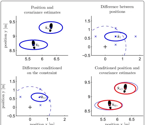
the prior to which the constraint is applied. See [72] for further details. The application of the constraint for the two-dimensional case is illustrated in Figure 6.
4.3 Inter-agent range measurement updates
Similar to the range constraint between the feet of an indi-vidual agent, the geometry of the inter-agent ranging gives the constraints
r−(γa+γb)≤ xa−xb ≤r+(γa+γb), (16) where r is the (true) range between agents’ ranging devices, andγa andγbare the maximum spatial separa-tion of respective ranging device and xa and xb, where in this case,xaandxbare the positions of a foot of each agent. The range only being dependent on xa − xb means that the state transformation z = T1x, where
1 =[1, 1, 1] and z1 = xa − xb, and the correspond-ing mean and covariance transformations as explained in the previous subsection can be used to let us exploit the marginalization (12).
Figure 6Illustration of the separation constraint update for two feet in the horizontal plane.The plots show (upper left) the prior position and covariance estimates, (upper right) the transformed system with the sigma points (blue crosses) and the constraint (dashed circle), (lower left) the projected sigma points and the conditional mean and covariance, and finally (lower-right) the conditioned result in the original domain with the prior covariances indicated with thinner lines.
The inter-agent ranging gives measurements r˜ of the ranger. As reviewed in Section 2.2, the malign attributes of r˜ which we have to deal with are potentially heavy-tailed error distributions and non-stationary spatially cor-related errors due to diffraction, multi-path, or similar. This can be done by using the model r˜ = r+ v+v, where vis a heavy-tailed error component, and v is a uniformly distributed component intended to cover the assumed bounded correlated errors in a manner sim-ilar to that of [75]. Combining the model with (16) and the state transformation T1 gives the measurement
model
˜
r−v−γr ≤ z1 ≤ ˜r−v+γr, (17)
whereγris chosen to cover the bounds in (16), the asyn-chrony betweenxˆaandxˆb, and the correlated errorsv. In practiceγrwill be a system parameter trading integrity for information.
To update the global state estimate with the the range measurement˜r, the statezˆ1and covariance estimatesPz1
must be conditioned on˜rvia (17). Due to the stochastic termv, we cannot use hard constraints as with the feet of a single agent. However, by assigning a uniform prior to the constraint in (17), the likelihood function ofr˜givenzˆ1
becomes
whereU(−γr,γr)is a uniform distribution over the inter-val [−γr,γr],V(ˆz1 − ˜r,σr)is the distribution ofvwith mean ˆz1 − ˜r and some scaleσr, and ∗denotes con-volution. Then, with the assumed Gaussian priorz1 ∼ N(zˆ1,Pz1), the conditional distribution ofz1 givenr˜,zˆ1,
andPz1is
f(z1|˜r)∝f(˜r|ˆz1)N(zˆ1,Pz1). (19)
Sincez1is low dimensional, the conditional moments ˆ
z1|˜r and Cz1|˜r can be evaluated by sampling. With
the marginalization (12) and the inverse transformation T−11, this will give the conditional mean and covariance ofx.
Since the likelihood function (18) is typically heavy tailed, it cannot easily be described by a set of sam-ples. However, since the prior is (assumed) Gaussian, the sampling of it can efficiently be implemented with the eigenvalue decomposition. With sample points u(i) of the standard Gaussian distribution, the corresponding sample points of the prior is given by
s(i)= ˆz1+Q1/2u(i),
where Pz1 = QQ is the eigenvalue decomposition
ofPz1. With the sample points s
(i), the associated prior
weights only become dependent onu(i)(apart from nor-malization) since
w(pri)∼e−12(s(i)−ˆz1)Pz−11(s(i)−ˆz1)=e−12u(i)2
and can therefore be precalculated. Reweighting with the likelihood function,w˜(poi) =wpr(i)·f(r˜|s(i))and normalizing
the weightsw(poi) = ˜w(poi)·(w˜(poi))−1, with suitable chosen u(i), the conditional moments can be approximated by
ˆ z1|˜r≈
i
w(poi)s(i) and Cz1|˜r ≈
i
w(poi)s(i)(s(i)).
Consequently, as long as the likelihood function can be efficiently evaluated, any likelihood function may be used. For analytical convenience, we have typically let V(·,·)
be Cauchy-distributed, giving the heavy-tailed likelihood function
f(r˜|s(i))∼atan
˜
r−s(i)+γr
σr
−atan
˜
r−s(i)−γr
σr
. (20)
The sampling-based range update with this likelihood function and u(i) from a square sampling lattice is
λ1/ 2 2 p2
λ1/ 2 1 p1
Prior
po
si
ti
o
n
y
[m]
position x [m]
0 5 10 0
5
10 Likelihood
position x [m]
0 5 10 0
5
10 Posterior
position x [m]
0 5 10 0
5 10
Figure 7Illustration of the suggested range update in two dimensions.From left to right, the plots show the Gaussian prior given by the meanzˆ1(blue dot) and the covariancePz1(blue ellipse), and with indicated samples (red dots) and eigenvectors/values, the (one-dimensional) likelihood function given by the range
measurement˜rand used to reweight the samples, and the resulting posterior with conditional meanzˆ1|rand covariancePz1|rcalculated
from the reweighted samples.
illustrated in Figure 7. Potential more elaborate tech-niques for choosing the sample points can be found in [103].
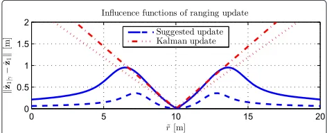
The presented ranging update gives a robustness to outliers in the measurement data. In Figure 8, the influ-ence functions for the sample-based update and the tra-ditional Kalman measurement update are shown for the ranging likelihood function (20) withγr =2 m andσr = 0.5 m, and position covariance values ofPz1 = Im2and Pz1 = 0.3I m2. By comparing the blue solid and the
red dashed-dotted lines, it is seen that when the posi-tion and ranging error covariances are of the same size, the suggested ranging update behaves like the Kalman update up to around three standard deviations, where it gracefully starts to neglect the range measurement. In addition, by comparing the blue dashed and the red dotted lines, it is seen that for smaller position error covari-ances, in contrast to the Kalman update, the suggested range update neglects ranging measurements with small errors (flat spot in the middle of the influence function).
Figure 8Influence functions for range updates forˆz1 =10m. The different functions correspond to the suggested method (blue solid/dashed lines) and a traditional Kalman measurement update (red dashed-dotted/dotted lines) withPz1=Im2andPz1=0.3Im2, respectively. For the suggested update,γr=2 m andv2were Cauchy distributed withσr=0.5 m, and for the Kalman measurement
0 100 200 300 400 500
Estimated trajectories from straigh-line march scenario
po
Figure 9Illustration of the gain of dual foot-mounted sensors and inter-agent ranging.The upper plot shows the step-wise dead reckoning of the individual feet (in blue and green) without any further information. The middle plot shows the step-wise dead reckoning with range constraints between the feet of the individual agents. The lower plot shows the complete cooperative localization with step-wise dead reckoning, range constraints, and inter-agent ranging.
This has the effect that multiple ranging updates will not make the position error covariance collapse, which captures the fact that due to correlated errors, during standstill, multiple range measurements will contain a diminishing amount of information; and during motion, the range measurements should only ‘herd’ the dead reckoning.
With slight modifications, the ranging updates can be used to incorporate information from many other infor-mation sources. Ranging to anchor nodes whose positions are not kept in x or position updates (from a GNSS
0 100 200 300 400 500
RMSE as a function of distance
RMSE absolute position RMSE relative position
Figure 10Absolute position RMSEs (blue lines) and relative position RMSEs (red lines) as functions of distance.The different blue lines correspond, in ascending order, to the increasing number of agents and are the results of 100 Monte Carlo runs. Clearly, the relative error is bounded by the inter-agent ranging while the absolute error grows slower the larger the number of agents. The final position RMSEs as a function of the number of agents are shown in Figure 11.
Figure 11Final position RMSEs as a function of the number of agents (blue crossed line).From the fit to 1/√N(dashed red line), the position error is seen to be decaying as the square root of the number of agents. The RMSEs are the results of 100 Monte Carlo runs.
receiver or similar) may trivially be implemented as range updates (zero range in the case of the position update) with z1 = xa −xb replaced withz1 = xa −xc, where xc is the position of the anchor node or the position
measurement. Fusion of pressure measurements may be implemented as range updates in the vertical direction, either relative to other agents or relative to a reference pressure.
4.4 Summary of sensor fusion
The central sensor fusion, as described in Section 3.3, keeps the position and heading of all feet in the global state vector x. From all agents, it receives dead reck-oning updates, [dp,dψ], Pp, Pp,ψ, and Pψ,ψ, and inter-agent range measurements r˜. The dead reckoning updates are used to propagate the corresponding states and covariances according to (7). At each dead reckon-ing update, the range constraint is imposed on the state space as described in subsection 4.2, and the correc-tions are sent back to the agent. The inter-agent range measurements are used to condition the state space as described in subsection 4.3. Pseudo-code for condition-ing the state mean and covariance estimates on the range constraint and range measurements is shown in Algorithms 2 and 3.
Algorithm 2 Pseudo-code for imposing the range con-straint (13), between navigation pointsxaandxb, on the global state estimatexˆ.
1: zˆ:=Tγxˆ and Pz:=TγPxTγ 2: L:=chol(Pz1)
3: Sample and project sigma points/weights
(z(1i),w(i))←(zˆ1,L)
4: zˆ1|γ :=iwiz(1i) and Cz1|γ :=
iwiz
(i)
1 (z
(i)
1 ) 5: Calculate conditional mean and covariance by
marginalization
(zˆ|γ,Pz|γ)←(zˆ1|γ,zˆ2,Cz1|γ,Pz)
6: xˆ|γ :=T−γ1zˆ|γ and Px|γ :=T−γ1Pz|γT−γ
Algorithm 3 Pseudo-code for conditioning the global state estimatexˆon the range measurements (17) between navigation pointsxaandxb.
1: zˆ:=T1xˆ and Pz:=T1PxT1 2: (Q,):=eig(Pz1)
3: s(i):= ˆz1+Q1/2u(i) ∀i 4: w˜(poi) :=wpr(i)·f(r˜|s(i)) ∀i 5: w(poi) := ˜w(poi)·(w˜(poi))−1 ∀i 6: zˆ1|˜r :=iw
(i)
pos(i) and Cz1|˜r:=
iw
(i)
pos(i)(s(i)) 7: Calculate conditional mean and covariance by
marginalization
(zˆ|˜r,Pz|˜r)←(zˆ1|˜r,zˆ2,Cz1|˜r,Pz)
8: xˆ|˜r:=T−11zˆ|˜r and Px|˜r:=T−11Pz|˜rT−1
−15 −10 −5 0 5 10 15 −10
−5 0 5 10
Estimated trajectory with 3 static agents
postion x [m]
po
st
io
n
y
[m
]
Figure 13Estimated trajectory from the scenario with three static agents and a fourth mobile agent.Clearly, the position estimation errors are bounded.
0 100 200 300 400 500 0
1
2 RMSE as a function of distance
distance [m]
er
ro
r
[m
]
Figure 14Position RMSEs of the mobile unit for the three static agents scenario.The RMSEs are the results of 100 Monter Carlo runs. Being static, the three stationary agents essentially become anchor nodes, and therefore, the RMSE is bounded.
5 Experimental results
To demonstrate the characteristics of the sensor fusion presented in the previous section, in the following subsec-tion, we first show numerical simulations giving a quanti-tative description of the fusion. Subsequently, to demon-strate the practical feasibility of the suggested architecture and sensor fusion, a real-time localization system imple-mentation is briefly presented.
5.1 Simulations
The cooperative localization by foot-mounted inertial sensors and inter-agent ranging is non-linear, and the behavior of the system will be highly dependent on the tra-jectories. Therefore, we cannot give an analytical expres-sion for the performance. Instead, to demonstrate the system characteristics, two extreme scenarios are simu-lated. For both scenarios, the agents move with 1 m steps at 1 Hz. Gaussian errors with standard deviation 0.01 m and 0.2° were added to the step displacements and the heading changes, respectively, and heavy-tailed Cauchy distributed errors of scale 1 m were added to the range measurements. The ranging is done time-multiplexed in a round-robin fashion at a total rate of 1 Hz.
OpenShoe units (foot-mounted inertial sensors)
USB hub
Ubisense radio tag (synthetic inter-agent ranging)
Android phone (proc. and com. device)
Figure 16Four agents with equipment displayed in Figure 15.The OpenShoe units are integrated in the soles of the shoes, and the radio tags are attached to the helmets. The cables and the USB hubs are not displayed.
5.1.1 Straight-line march
Nagents are marching beside each other in straight lines with agent separation of 10 m. The straight line is the worst case scenario for the dead reckoning, and the posi-tion errors will be dominated by errors induced by the heading errors. In Figure 9, examples of the estimated trajectories of the right (blue) and left (green) feet are shown from three agents without any further informa-tion, with range constraints between the feet and with range constraints and inter-agent ranging. The absolute and relative root-mean-square error (RMSE) as a function of the walked distance, and for different number of agents, are shown in Figure 10. The relative errors are naturally bounded by the inter-agent ranging. However, the heading
RMSE grows linearly with time/distance, and therefore, the absolute position error is seen to grow with distance. Similar behavior can be observed in the experimental data in [64,91]. Naturally, the heading error and therefore also the absolute position RMSE drop as 1/√N, where N is the number of agents. This is shown in Figure 11. We may also note that the position errors of the different agents become strongly correlated. The correlation coefficients for two agents as a function of distance are shown in Figure 12.
5.1.2 Three static agents
Three non-collinear agents are standing still. This will be perceived by the foot-mounted inertial navigation, and
therefore, they essentially become anchor nodes. This is obviously the best-case scenario. A fourth agent walks around them in a circle. An example of an estimated tra-jectory is shown in Figure 13, and the RMSE as a function of time is shown in Figure 14. Since anchor nodes are essentially present in the system, the errors are bounded. See [104] for further discussions. The non-zero RMSE reflects the range constraints in the system.
From the two scenarios, we can conclude that the rel-ative position errors are kept bounded by the inter-agent ranging, while the absolute position errors (relative start-ing location) are bounded in the best case (stationary agents) and that the error growth is reduced by a factor of 1/√Nin the worst case.
5.2 Real-time implementation
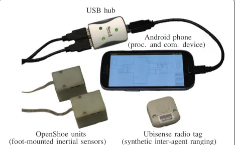
The decentralized system architecture has been realized with OpenShoe units [15] and Android smartphones and tablets (Samsung Galaxy S III and Tab 2 10.1, Samsung Electronics Co., Ltd., Suwon, Korea) in the in-house developed tactical locator system TOR. The communi-cation is done over an IEEE 802.11 WLAN. Synthetic inter-agent ranging is generated from position measure-ments from a Ubisense system (Ubisense Research & Development Package, Ubisense Group plc., Cambridge, UK), installed in the KTH R1 reactor hall [105]. The intension is to replace the Ubisense system with in-house developed UWB radios [26]. The equipment for a single agent is shown in Figure 15. The multi-agent setup with additional equipment for sensor mounting is shown in Figure 16.
The step-wise inertial navigation and the associated transfer of displacements and heading changes have been implemented in the OpenShoe units. The agent filtering has been implemented as Android applications together with graphical user interfaces. A screenshot of the graphi-cal user interface with trajectories from a∼10-min search in the reactor hall and adjacent rooms (built-up walls not displayed) by three smoked divers is shown in Figure 17. The central sensor fusion has been implemented as a separate Android application running on one agent’s Android platform. Recently, voice radio communication and 3D audio have been integrated into the localization system [106].
6 Conclusions
Key implementation challenges of cooperative localiza-tion by foot-mounted inertial sensors and inter-agent ranging are designing an overall system architecture to minimize the required communication and computa-tional cost while retaining the performance and making it robust to varying connectivity, and fusing the informa-tion from the system under the constraint of the system architecture while retaining high integrity and accuracy.
A solution to the former problem has been presented in the partially decentralized system architecture based on the division and physical separation of the step-wise inertial navigation and the step-wise dead reckoning. A solution to the latter problem has been presented in the marginalization and sample-based spatial separation con-straint and ranging updates. By simulations, it has been shown that in the worst case scenario, the absolute local-ization RMSE improves as the square root of the number of agents, and the relative errors are bounded. In the best case scenario, both the relative and the absolute errors are bounded. Finally, the feasibility of the suggested architec-ture and sensor fusion has been demonstrated with sim-ulations and a real-time system implementation featuring four agents and a meter-level accuracy for operation times of tenth of minutes in a harsh industrial environment.
Competing interests
The authors have no connection to any company whose products are referenced in the article. The authors declare that they have no competing interests.
Acknowledgements
Parts of this work have been funded by the Swedish Agency for Innovation Systems (VINNOVA).
Received: 30 May 2013 Accepted: 14 October 2013 Published: 29 October 2013
References
1. J Rantakokko, J Rydell, P Strömbäck, P Händel, J Callmer, D Törnqvist, F Gustafsson, M Jobs, M Grudén, Accurate and reliable soldier and first responder indoor positioning: multisensor systems and cooperative localization. IEEE Wireless Commun.18, 10–18 (2011)
2. C Fuchs, N Aschenbruck, P Martini, M Wieneke, Indoor tracking for mission critical scenarios: a survey. Pervasive and Mobile Comput.7, 1–15 (2011) 3. K Pahlavan, X Li, J Makela, Indoor geolocation science and technology.
IEEE Commun. Mag.40(2), 112–118 (2002)
4. V Renaudin, O Yalak, P Tomé, B Merminod, Indoor navigation of emergency agents. Eu. J. Navigation.5, 36–42 (2007)
5. G Glanzer, Personal and first-responder positioning: state of the art and future trends, inUbiquitous Positioning, Indoor Navigation, and Location Based Service (UPINLBS), (Helsinki, Finland, 3–4 Oct 2012)
6. C Fischer, H Gellersen, Location and navigation support for emergency responders: a survey. IEEE Pervasive Comput.9, 38–47 (2010) 7. J Hightower, G Borriello, Location systems for ubiquitous computing.
Computer.34(8), 57–66 (2001)
8. M Angermann, M Khider, P Robertson, Towards operational systems for continuous navigation of rescue teams, inIEEE/ION Position, Location and Navigation Symposium (PLANS), (5–8 May 2008)
9. A Mourikis, S Roumeliotis, On the treatment of relative-pose measurements for mobile robot localization, inIEEE International Conference on Robotics and Automation, (Orlando, FL, USA, 15–19 May 2006)
10. R Harle, A survey of indoor inertial positioning systems for pedestrians. IEEE Commun. Surv. Tutor.PP(99), 1–13 (2013)
11. E Foxlin, Pedestrian tracking with shoe-mounted inertial sensors. IEEE Comput. Graph. Appl.25, 38–46 (2005)
12. J Rantakokko, E Emilsson, P Strömbäck, J Rydell, Scenario-based evaluations of high-accuracy personal positioning systems, inIEEE/ION Position, Location and Navigation Symposium (PLANS), (Myrtle Beach, SC, USA, 23–26 Apr 2012)