R E S E A R C H
Open Access
mm-Wave channel estimation with
accelerated gradient descent algorithms
Hossein Soleimani
1, Danilo De Donno
2and Stefano Tomasin
1,3*Abstract
The availability of millimeter wave (mm-Wave) band in conjunction with massive multiple-input-multiple-output (MIMO) technology is expected to boost the data rates of the fifth-generation (5G) cellular systems. However, in order to achieve high spectral efficiencies, an accurate channel estimate is required, which is a challenging task in massive MIMO. By exploiting the small number of paths that characterize the mm-Wave channel, the estimation problem can be solved by compressed-sensing (CS) techniques. In this paper, we propose a novel CS channel estimation method based on the accelerated gradient descent with adaptive restart (AGDAR) algorithm exploiting a1-norm
approximation of the sparsity constraint. Moreover, a modified re-weighted compressed-sensing (RCS) technique is considered that iterates AGDAR using a weighted version of the1-norm term, where weights are adapted at each iteration. We also discuss the impact of cell sectorization and tracking on the channel estimation algorithm. We compare the proposed solutions with existing channel estimations with an extensive simulation campaign on downlink third-generation partnership project (3GPP) channel models.
Keywords: Compressed sensing, Estimation, mm-Wave
1 Introduction
Due to its huge spectrum availability, the millimeter wave (mm-Wave) band is currently considered for the fifth gen-eration (5G) of cellular networks [1–3]. The high atten-uation incurred at those frequencies imposes the use of multiple antennas at each device, typically resulting in massive multiple-input-multiple-output (MIMO) sys-tems, giving rise to various challenges. We focus here on channel estimation that is needed for proper transmit beamforming. In fact, the least square (LS) estimate using short training sequences and limited transmit power (to reduce overhead in massive MIMO systems) is not accu-rate enough for capacity achieving beamforming. How-ever, the mm-Wave MIMO channel comprises a small number of dominant clusters of paths and even with many antennas a small set of parameters characterizes the entire channel. This induces a sparsity of the mm-Wave channel matrix when transformed by a Fourier transform into the
*Correspondence:[email protected]
1Department of Information Engineering, University of Padova, via Gradenigo 6/A, Padua, Italy
3Consorzio Nazionale Interuniversitario per le Telecomunicazioni, Padua, Italy Full list of author information is available at the end of the article
so-called virtual channel, and compressed-sensing (CS) techniques can be used for channel estimation.
Various solutions have been proposed for channel esti-mation in mm-Wave communication systems, and the reader may refer to [4] for their survey. Part of the litera-ture has considered transceivers with hybrid beamformers (cascade of beamformers before and after the digital to analog converters): the joint optimization of both train-ing and estimation has been pursued in [5] for these structures using a feedback channel. Orthogonal match-ing pursuit (OMP) solutions have been considered with both single path [6,7] and multiple-path cancelation [8,9]. In [10], an enhanced approach for generating the beam-forming codebook has been proposed, using the contin-uous basis pursuit (CBP) method, while [11] considers a fast iterative shrinkage-thresholding algorithm (FISTA) approach.
For fully digital beamformers, [12] considers the sparse channel estimation as a least absolute shrinkage and selec-tion operator (LASSO) problem. In [13], OMP is used to estimate the channel by iteratively detecting and cancel-ing paths from the virtual channel estimate. In [14], a basis pursuit denoise (BPDN) approach is suggested where a weighted version of 1-norm term is considered in the
LASSO problem and weights are iteratively adapted. A sparsity adaptive matching pursuit (SSAMP) approach is instead used in [15], while in [16] the LASSO problem is solved by applying a generalized approximate mes-sage passing (GAMP) algorithm exploiting the Bernoulli-Gaussian distribution of paths in the virtual channel.
In this paper, we propose a novel sparse channel esti-mation method based on the accelerated gradient descent with adaptive restart (AGDAR) algorithm [17]. Focus-ing on a scenario where the receiver obtains first the LS estimate of the narrowband mm-Wave MIMO chan-nel, we relax the sparse optimization problem using LASSO, wherein the0-norm is replaced by the1-norm. We apply then the AGDAR algorithm [17] to solve the sparse channel estimation problem. In order to further enhance the channel estimation procedure, a re-weighted
1-norm problem is considered leading to the re-weighted compressed-sensing (RCS) algorithm [18], which iterates AGDAR with different weights of the1-norm term. We also discuss the impact of cell sectorization and chan-nel tracking on the chanchan-nel estimation algorithm. We compare the proposed solutions with OMP solutions [6, 8, 13]. With respect to the rest of the literature we reduce the complexity (with respect to the random search of A-LASSO in [12]), we swap the objective functions and the constraints with respect to [14], effectively minimiz-ing the mean square error (MSE) and providminimiz-ing details on the implementation of the optimization algorithm. Com-pared to [15], we use different algorithms (AGDAR and RCS instead of SSAMP) that trade-off between sparsity and noise reduction. Lastly, we consider a single user and a static pilot transmission for the initial estimate, while [16] considers the adaptation of the transmit and receive beamformers to allow channel estimation simulta-neously for more users. An extensive simulation campaign on third-generation partnership project (3GPP) channel models [3] for a downlink scenario has been conducted to show the merits of the proposed approach in terms of both estimate MSE and computational complexity.
The rest of the paper is organized as follows. We intro-duce the system model in Section2, providing the descrip-tion of both the mm-Wave channel model and the existing OMP solutions. The sparse channel estimation problem is introduced in Section3, together with a discussion on sec-torization and channel tracking. The proposed AGDAR technique is described in Section 4, together with the refined RCS approach. Numerical results are presented in Section5to assess the performance of the considered techniques in a 5G scenario, before conclusions are driven in Section6.
2 System model
We consider a massive MIMO narrowband communica-tion system withNt antennas at the transmitter andNr
antennas at the receiver. This models indifferently either the uplink or the downlink of a cellular communication system. LetH∈CNr×Ntbe the channel matrix with
com-plex entries. Antennas are organized into either uniform linear arrays (ULAs) [19] or uniform planar arrays (UPAs) [20] at both the transmitter and receiver: ULA antennas are uniformly spaced along thez axis while UPA anten-nas are uniformly tiled over the yz-plane1. For the sake of a clearer explanation in the main body of the paper, we only provide derivations for ULA, while we report in
AppendixAthe results for an UPA withD2×D3 = Nt
transmit antennas andD0×D1=Nrreceive antennas. We indicate withLthe number of paths for the signal from the transmitter to the receiver, so that the channel matrix entries can written as
[H]i1,i2= spacing, and αl is the l-path amplitude including path
loss, shadowing, and fading. Note that parametersηldare related to the angles of departure and arrival of the l -th pa-th. By assumingδ ≤ λ/2, we have ηld ∈ −12,12. The statistics of each parameter depend on the considered propagation scenario, and various relevant cases can be found for example in the 3GPP mm-Wave channel model [3] including channel models with clustered sub-paths [3], whereLbecomes the total number of (sub-)paths from all clusters. Typically, in mm-Wave systems, the number of paths (or sub-paths)Lis small [21].
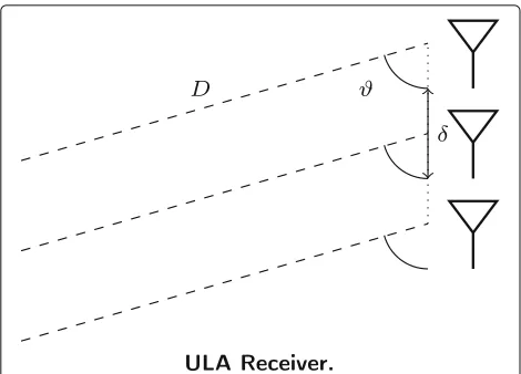
Figure 1 shows an example of receiver with Nr = 3
receive antennas and a single path arriving at the anten-nas with an angleϑfrom a distanceD: in this caseη11 =
The considered channel estimation techniques in this paper are all based on the LS channel estimate, briefly summarized here.
The set ofNttraining symbols2transmitted with theNt antennas are collected into theNt×NtmatrixS, assumed here to be unitary. The corresponding receivedNt×Nr matrix signal is
R=HS+N, (2)
whereN ∈ CNr×Nt is the noise matrix with independent
and identically distributed (iid) zero-mean complex Gaus-sian entries, each with powerσ2. The LS channel estimate at the receiver is obtained as [22]
Fig. 1ULA receiver. Single path received by ULA withNr=3 antennas at distanceDfrom the source. In this caseη1
1= δλcosϑand
α1=D12e−j2π
D
λ
whereNis a matrix with iid zero-mean complex Gaussian entries having power σ2 (thanks to the unitary prop-erty ofS). Note that this estimation procedure may yield a significant overhead for the transmission of training sequences only when the number of transmit antennas grows large [23], since the number of transmitted sym-bols (the columns ofS) isNt. We will further address this problem in Section3.
2.2 OMP methods
We will compare our channel estimation algorithm with two OMP techniques: single peak cancelation (SPC) [6] and joint peak cancelation (JPC) [8]. Both methods use the Fourier transform of the channel matrix, in what is usually denoted asvirtual channelorangular domain rep-resentation [24, Sec. 7.3.3]. With reference to ULA, let In(x)= nsinsin(π(πxx)
n)
be the 1D-periodic sinc function and let
[W
be the two-dimensional (2D) sampled periodic sinc
func-tion, whereM1 andM2 are the number of samples per
period in the 2D virtual channel domain, f = (f1,f2), discrete Fourier transform (DFT) ofHwith entries [6]
[V]f =
The SPC method [6] reported in Algorithm 1 (foralgo = SPC), iteratively estimates the amplitudeαland the
dis-cretepositions l of I paths in the virtual channel and cancels their corresponding periodic sinc functions in the virtual channel. After I iterations, the channel esti-mate H is obtained by taking the 2D-inverse discrete Fourier transform (IDFT) of the estimated virtual channel
V reconstructed by summing the contributions of all the detected paths.
Algorithm 1SPC and JPC channel estimation methods Input: H,I,algo
MSE of the channel estimate. Note that SPC provides an intrinsically approximated solution even in the absence of noise, since the peak positionslare estimated on a fixed discrete grid.
The JPC algorithm of [8] reported in Algorithm 1 (for algo=JPC) is a modification of SPC that at each iteration jointly estimates the amplitudes of all previously detected peaks by the LS approach and cancels the corresponding periodic sinc’s from the virtual channel. In particular,x=
vec(X)stacks the columns of matrix Xinto the column vector x; at iterationl, one peak is detected (line 3) and then the amplitudes of all previously detected peaks are jointly estimated (line 8), and the new virtual channel with removed peaks is obtained (lines 9–11). This is achieved by building matrixwthat contains in columnlthe vector version ofW
l(line 6).
This algorithm has the advantage over the SPC that each amplitude estimate is refined at each iteration thus taking advantage also of the peaks detected in further iterations.
3 Sparse dual channel estimation
In order to obtain an efficient and simple channel esti-mator, we exploit the specific channel structure described in the previous section. In particular, we use the fact that the channel is composed of a small number of paths with respect to the typically large number of transmit and receive antennas.
In this paper, we directly refer to the representation (1) and interpret it as 2D-IDFT of a sparse matrix having only Lnon-zero entries. First, the channelHis rearranged into the channel column vectorh = vec(H) ∈ CNrNt×1with entries
[h]i1+Nri2=[H]i1,i2, (6)
wherei1 = 0,. . .,Nr −1,i2 = 0,. . .,Nt−1, while the 2D-IDFT matrix isF ∈CNtNr×M2M1with entries
[F](i1+Nri2,f1+M1f2)=
column vectorvof lengthM1M2withLnon-zero entries at position¯l1+M1¯l2, forl=1,. . .,L, i.e., approximate the channel vector as
h≈Fv. (10)
We will denote withvas the dual channel in theM1×M2 domain. Note that the dual channel is sparse as it contains onlyLnon-zero entries.
Remark 1The approximation (10) stems from the rounding of (9), i.e., from approximatingld with¯ld. As Md → ∞, the approximation becomes more accurate.
Moreover, we have used DFTs with Mdpoints along
dimen-sion d, as for the dual channel representation, in order to make a simpler comparison among various channel esti-mation schemes. Lastly, note that v is not the vectorial representation of the virtual channel, since the DFT used to obtain the virtual channel does not invert the IDFT of (10): in fact, the DFT is taken on the reduced set of Nr×Nt samples, thus yielding the periodicsinc’s of (4).
Similarly to the vectorial representation of the channel, we define
h=vec(H)≈Fv+n, (11)
where indices ofH to obtainhare selected similarly to (6). From (11), we observe that the LS estimate is a noisy version of a linear transformation of the dual channelv.
We propose an algorithm that improves the LS channel estimate by exploiting the sparsity ofv. In particular, we define byvˆ the new estimate of the dual channelvand write the sparse channel estimation problem as
v=argmin
v
Fv−h22+ρv0, (12)
wherev0is the0-norm that counts the non-zero ele-ments invandρis a parameter that controls the sparsity of the solution. This problem formulation aims at mini-mizing the MSE between the estimated channel and the LS channel estimate, under a constraint on the sparsity of vectorvˆ, imposed by the norm-zero term.
Unfortunately, problem (12) is non-convex and NP-hard [25]. Thus, we relax the problem by replacing the0-norm with the1-norm obtaining the LASSO problem
v=argmin
4 Solution of the sparse channel estimation problem
A vast literature is available for the solution of the sparse channel estimation problem (13), see for example the sur-vey [26]. We propose here to use two recent and efficient methods based on the gradient descent algorithm with improved convergence speed, namely the AGDAR algo-rithm (also named FISTA with adaptive restart [27]) and the RCS algorithm [18].
4.1 Accelerated gradient descent with adaptive restart
The AGDAR algorithm [27] has been developed to solve problems where the objective function is the sum of a differentiable function and a general but simple closed convex function.
Here, we briefly summarize the motivation of the AGDAR algorithm. We first observe that the minimiza-tion problem minx∈RNf(x) when f(·) is convex and
smoothcan be solved by the gradient descent algorithm that iteratively updates the solution, computing at itera-tionp
xp=xp−1−t∇f(xp−1), (14)
where t is the step size and ∇f(x) is the gradient of f(·)computed inx. An alternative formulation of (14) is provided by theproximal form[28]
xp=argminx∇f(xp−1)T(x−xp−1)+ convex and smooth but g(·) convex, nondifferentiable, and lower semicontinuous, the proximal form must be modified as follows [28]
xp=argminx∇f(xp−1)T(x−xp−1)+
In general, this optimization problem may be hard to solve; however, when g(x) = ρ||x||1, problem (16) is efficiently solved by splitting it into N separate one-dimensional problems for each entry of x ∈ RN, i.e.,
[xp]n=argminxρ|x| +
obtaining the iterative shrinkage-thresholding algorithm (ISTA) algorithm. This solution can be made faster by applying the Nesterov acceleration principle [30]: instead
of using the gradient descent (14),xpis updated as a
lin-ear combination of the gradient descent terms (14) at the current and previous iterations, i.e.,
yp=xp−1−t∇f(xp−1), (19a)
xp=(1−γp−1)yp+γp−1yp−1. (19b)
Combining this approach with ISTA, we obtain the FISTA algorithm where [yp]n= Tρt(zn)andxpis updated using
(19b) It turns out that this approach fastens the conver-gence of the algorithm for example by choosing as linear combination coefficients [30]
γp=
The explanation of the Nesterov iteration is not very intuitive, and the interested reader can find more details in [30].
The parameter choice (20) is not in general optimal while its optimization is a difficult task. An alternative approach is theadaptive restarttechnique [27], in which
γpis set according to (20) (thus in a suboptimal way) but
the FISTA algorithm is restarted whenever the objective function is locally increasing (thus the iterative solution is moving in the wrong direction), i.e., when
∇f(xp−1)T(yp−yp−1) >0 , (22) From (19a) we obtain that the restarting condition (22) can be written as
(xp−1−yp)(yp−yp−1) >0 . (23) The restart consists in resettingθp = 1 and using as
initial point the last point produced by the algorithm.
4.2 Re-weighted compressed sensing
The RCS method is proposed [18] to improve the spar-sity of the gradient descent solution of (13). The algorithm weights the entries ofxpin the1-norm in (13) in order to better approximate the0-norm term in (12). Therefore, instead of solving (12), the RCS method aims at solving problem
Algorithm 2AGDAR algorithm
As the0-norm counts the non-zero entries, regardless of their amplitude, for non-zero weights, the two problems (12) and (25) have the same solutions.
About the choice of the weights, they are meant to provide a good approximation of the0-norm using the (weighted)1-norm. Therefore, imposing that at solution
Dvˆ1= ˆv0, (26)
we obtain the optimum weights (diagonal entries of matrixD)
where∗denotes any non-zero value. However, this choice requires the knowledge of the problem solutionvˆ, which is not available while solving the problem.
In [18], an iterative approach has been proposed, where the weights are adapted to converge to (27) without know-ing the optimal solution. In particular, RCS runsq2times the AGDAR algorithm, using at each iteration a differ-ent set of weights chosen according to (28). It has been shown by extensive simulations over a variety of examples that the following weight adaptation strategy is perform-ing well: startperform-ing fromD0 = diag{[ 1,. . ., 1]}, for which
small number. Note that at convergence (forζ ≈ 0) we obtain (27).
Algorithm 3RCS algorithm Input: h,ρ,,q1,q2,tandζ
The implementation of RCS is obtained by runningq2 times the AGDAR algorithm and computing the shrinkage function with a weighted parameter, i.e., Twnρt(zn). The resulting procedure is reported in Algorithm 3.
It has been shown [18] that the RCS algorithm is a majorization-minimization algorithm that iteratively min-imizes a simple surrogate function majoring the objective function, and indeed provides in general a better approxi-mation to the original0-norm problem.
4.3 Sectorization and channel tracking
When the antennas at either or both the transmitter and the receiver are transmitting/receiving in a focused direction (in what is known as cell sectorization), the departure and arrival angles are within sub-intervals of [ 0, 2π); therefore, alsoηldwill take value in sub-intervals
. Therefore, vector v can be reduced by eliminating the entries corresponding to val-ues ofηldthat are never taken by the channel realization. Correspondingly, the columns ofF are removed and the AGDAR algorithm is run over a reduced space, thus increasing its accuracy.
more effective by simply tracking its changes rather than starting from scratch its estimation. We propose to focus the search of the paths in the dual channel within inter-vals around the initial estimates of arrival and departure angles. Therefore, for both AGDAR and RCS approaches, we have a reduction of the dual channel vectorv. Indeed, this is similar to sectorization; however, for channel track-ing we must consider multiple angle intervals, one for each initially estimated path.
Sectorization or tracking are also possible for SPC and JPC, wherein the search of the peak positionslwill be done on a sub-grid of theM1×M2grid, according to the intervals ofηl1andηl2. Also in this case, the benefits for the channel estimation process will be a lower probability of periodic sinc misplacement, as the search space is smaller.
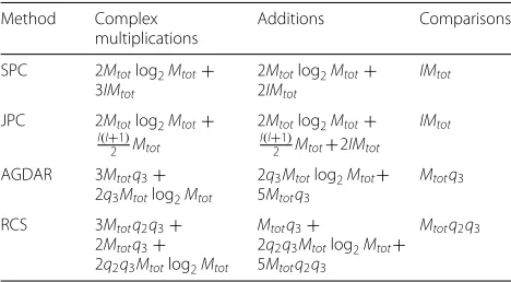
4.4 Computational complexity
The computational complexity of the considered algo-rithms is evaluated in terms of complex multiplications (CMUX), complex additions (CADD), and comparisons (COM). LetMtot = dMd, where the product is along
all dimensions, depending on the use of either UPA or ULA. Hence, using the fast Fourier transform algorithm, a (I)DFT ofMtotsamples requiresMtotlog2MtotCMUX,
Mtotlog2MtotCADD and no comparison. A summary of
the computational complexity of the various algorithms is reported in Table 1, where q3 denotes the effective number iterations over the variablepof the AGDAR and RCS algorithms. In the following section, we will present numerical results also for a complexity comparison among the various techniques.
5 Numerical results
In this section, we compare the proposed channel estima-tion techniques by evaluating the MSE in decibels (dB)
MSE=10 log10E||H−H||22, (29)
whereE[·] denotes the expectation operator andHˆ is the estimated channel matrix.
Table 1Computational complexity of the channel estimation methods
We consider the urban macro cell (UMa), urban micro cell (UMi), rural macro cell (RMa), and Indoor Hotspot (InH) 3GPP channel models [3], with both line-of-sight (LOS) and non-line-of-sight (NLOS). In these scenarios, the number of clusters (typically from 4 to 20) depends on the channel model and the number of sub-paths is 20 per cluster, thus totalingLin the range of tens to hundreds. Note that although the number of sub-paths is large, only three or four sub-paths have a notable power. Therefore de facto, we find the sparse channel model described in this paper and in many literature papers and measurement campaign results. Channels are obtained for a downlink, where the base station (BS) and user equipment (UE) are on the same plane, with parameters defined in Table2. The average channel gain is unitary, so we assume that transmit power has been adapted to compensate for the path loss; therefore, the average SNR is the reciprocal of the noise power. This also provides that the MSE for the LS estimate is simply the reciprocal of the SNR, which is then not reported in the figures.
For the proposed AGDAR and RCS algorithms, we use parameters as in Table2. In the following, we will always consider the same antenna geometry (either ULA or UPA) at both BS and UE, with a different number of antennas at the two ends.
5.1 Parameters setting
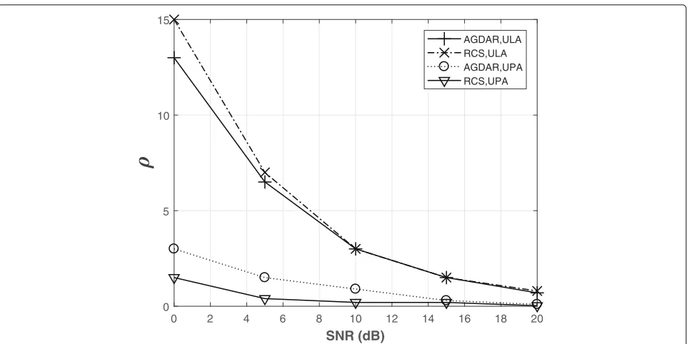
We first evaluate the impact of the parameters on the channel estimate MSE. The performance of both AGDAR and RCS is determined by the parameterρ that weights the1-norm term in the objective function and should be chosen according to the channel sparsity and the oper-ating signal to noise ratio (SNR). For each value of SNR, we have assessed the optimum value ofρthat minimizes the average MSE of the channel estimate. The results are reported in Fig. 2for both (at both devices) with Nr =
16 = 4 × 4 (D0 = D1 = 4) and Nt = 4 = 2 ×2
Table 2Simulation parameters
Parameter Value
number of sub-paths per cluster 20
BS position (0, 0)m
BS antenna altitude 25 m
UE position (90, 15)m
UE antenna altitude 1.5 m
Carrier frequency f=28 GHz
δ λ/2
Average channel gain 0 dB
10−6
q2 3
0 2 4 6 8 10 12 14 16 18 20
SNR (dB)
0 5 10 15
AGDAR,ULA RCS,ULA AGDAR,UPA RCS,UPA
Fig. 2Choice ofρ. Optimized value ofρvsSNR, for both UPA, withNr=16=4×4 (D0=D1=4) andNt=4=2×2 (D2=D3=2) and M0=M1=M2=M3=8, and ULAs withNr=16,Nt=4 andM1=M2=32. UMi LOS model
(D2 = D3 = 2) andM0 = M1 = M2 = M3 = 8, and
ULAs (at both devices) withNr = 16,Nt = 4 andM1 = M2= 32. In this case the channel model is UMi LOS for which the number of clusters is random, between 3 and 12, while the number of sub-paths per cluster is 20, for a
maximum total ofL = 240 paths. We can see a smooth
behavior ofρwith respect to the average SNR, that can be described with simple functions for its adaptation to oper-ating conditions. Moreover, as the average SNR increases, the optimalρdecreases, since the LS estimate is less noisy and a limited sparsification of the channel is required. We have optimized the value of this parameter also for other conditions (e.g., different number of antennas) and forthcoming results are obtained with the optimizedρ.
A second relevant parameter for both AGDAR and RCS is the maximum number of iterationsq1. Figure3shows the average MSE as a function of the number of maximum allowed iterationsq1for ULAs withNr=16,Nt=4, and various DFT sizes. We note that for all DFT sizes the MSE is flooring asq1increases: in particular, with log10q1 = 2.5, all algorithms converge to the minimum MSE. We also observe that the required number of iterations grows with
(M1,M2), and RCS achieves a lower asymptotic MSE and converges faster.
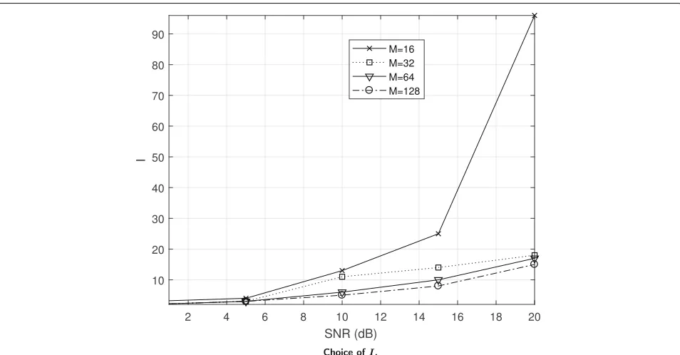
For a comparison with SPC and JPC, we have also opti-mized parameter I, i.e., the number of detected paths. Note that the existing literature typically assumes the knowledge ofLand setsI = L. We instead observe that Idoes not necessarily correspond to the number of paths,
since small paths can be neglected as may be easily con-fused with noise artifacts. This is particularly true in the 3GPP channel model, where many clusters and sub-paths are present, most of which however have a very limited power. Figure 4shows the value ofI that minimizes the average MSE versus the average SNR for various values of M = M1 = M2, using ULAs withNr = 16,Nt = 4 and SPC. The channel model is UMi LOS. We observe that we need a large value ofIwhen the SNR is high, as the con-sidered channel model has many (sub-)paths, and at high SNRs, they can be distinguished from the noise. Also, note that the optimal value ofIis decreasing as Mincreases: indeed, for higher M the approximation between posi-tionslandˆl becomes more accurate, thus fewer sinc
functions (closer to the actual number of paths) is enough (and better) for channel estimation. The results reported in the rest of this section are obtained with the optimized value ofI.
Lastly, we consider the optimization of the DFT size, i.e., the number of points used to approximateηld in all con-sidered channel estimation methods. In AppendixB, we provide the analytical derivation of the MSE as a func-tion ofM, for ULA and a Rayleigh fading channel with a small number of taps. Figure5shows the MSE as a func-tion ofM=M1=M2for ULA withNt=8,Nr =2 and the channel model described in AppendixB. As expected the MSE decreases for a higher value ofM, as the quan-tization error is reduced, flooring for high values of M.
Fig. 3Effects of iterationsq1. MSE vs the maximum number of iterationsq1for ULA withNr=32,Nt=4 using AGDAR (solid lines) and RCS (dotted lines). UMi LOS model
andNt = 4 and a DFT size multiple μ of the number
of antennas, i.e.,M1 = μNrandM2 = μNt. For a UMi LOS model, Fig.6shows the average MSE for an SNR of 0, 10, and 20 dB, and different channel estimation tech-niques. We observe that in all cases by increasingμ we obtain a better channel estimate, thanks to a better quan-tization precision of either the virtual channel domain (for
SPC and JPC) or the values ofηld (for both AGDAR and RCS). Moreover, both AGDAR and RCS methods achieve a lower MSE than SPC and JPC techniques at both low and high SNRs, thanks to their better exploitation of compact channel representation in the dual domain. The RCS has almost negligible performance improvement with respect to AGDAR, as both have a gain from 3 to 5 dB with respect
Fig. 5Analysis of choice ofM. MSE vsM=M1=M2for the scenario of AppendixB, withNt=16 andNr=4
to interference cancelation techniques. Note that the gain is more remarkable at a lower SNR, showing that the compressed-sensing techniques are able to better reject the noise. Lastly, note that JPC has an almost negligible improvement over SPC; thus, we can conclude that the detection of the peaks is already accurate when performed
sequentially rather than in parallel. Overall, we conclude thatμ=2 already provides close-to-optimal results for all methods. Similar observations can be drawn from Fig.7, where we report the MSE for a UPA configuration with 2×2 antennas at the UE and 6×6 antennas at BS in a UMa LOS channel model.
Fig. 7Choice ofMforNr=32 andNt=4. MSE vsμfor UPA withNr=36 andNt=4 at an SNR of 0 (dotted lines), 10 (solid lines) and 20 dB (dashed lines) andM1=μNrandM2=μNt. UMa LOS model
In order to show the performance of the proposed solution in a scenario with a large number of antennas, Fig. 8 shows the MSE as a function ofμ for ULA with
Nr = 128 and Nt = 16 and the UMi LOS model.
Also in this case, we can appreciate the advantage of all
techniques with respect to the LS method, as we recall that for LS the MSE is the reciprocal of the SNR, thus 0 dB in correspondence of the dotted lines, −10 dB for the solid lines and−20 dB for the dashed lines. Indeed, a higher number of antennas with respect to Fig.6increases
the gain of the other channel estimation techniques with respect to LS. About the comparison among the various methods, we can derive similar conclusions as those of Fig.6, confirming also that other results are representative of a massive MIMO scenario.
5.2 Sectorization and channel tracking
As we already discussed, sectorization provides a faster and more accurate search of the channel paths. Here, we consider a system where channel angles are uniformly dis-tributed in intervals of 6, 60, and 180 degrees. We have
L = 14 paths, with independent Gaussian-distributed
amplitudes αl: by this simple channel model, we better
capture the effects of sectorization and channel tracking. Figure9shows the resulting MSE as a function ofM= M1=M2for the various systems, when the average SNR is 10 dB. We observe that sectorization indeed reduces the MSE of all channel estimates, and sectors of 6◦ pro-vide a MSE of 10 to 16 dB smaller than that of 6◦sectors. Comparing the various techniques we observe that with large (180◦) and small (6◦) sectors all techniques take advantage of the sectorization in a similar way, while for intermediate values (60◦) the compressed-sensing meth-ods have a higher gains than interference cancelation methods.
We also consider channel tracking where, after an ini-tial channel estimation performed according to the var-ious considered techniques and with an angle span of
360◦, when channels are time-invariant. Estimators are run using an angle span of 6◦around the angles of each path. Figure10shows the MSE of the channel estimates at an average SNR of 10 dB, and for various values of M1andM2. We observe that, thanks to the search over a smaller angle span both SPC and JPC achieve similar performance to the proposed approaches, a phenomenon that we already observed with sectorization. Also, the dif-ference between RCS and AGDAR is further reduced, again because of the easier task of channel estimation in this case. We still note instead a high sensitivity to the DFT-size, which corresponds to an accuracy in the esti-mate of the angles of arrival and departure. Lastly, both sectorization and channel tracking reduce the complexity of the proposed solutions, as path search operations can be performed on a reduced space.
5.3 3GPP channel scenarios comparison
Until now, we considered only the UMi LOS channel model: in this section instead, we consider also the other 3GPP channel models. Figure11shows the average MSE for various algorithms and UPAs withNt = 8×8 at the
BS and Nr = 2 ×2 at the UE, and M0 = M1 = 10
andM2 = M3 = 4. We compare various channel
esti-mation techniques for an average SNR of 10 dB. At this intermediate SNR value, we observe that the proposed AGDAR and RCS significantly outperform both SPC and JPC for all the considered channel models, by 6 to 7 dB.
Fig. 10Effects of tracking. MSE for ULAs of various channel estimation techniques, when the average SNR is 10 dB with channel tracking at 6◦, and various values ofM.Nr=16 andNt=4
The indoor-office model (InH Mixed) has a few signifi-cant taps with reduced dispersion, a favorable condition for SPC and JPC, which exhibit a reduced gap with respect to the proposed (still better performing) techniques. On the other hand, dispersive channels with many low-power
taps (UMi Street Canyon NLOS) make the channel esti-mation more problematic for SPC and JPC, while can be handled very efficiently by the compressed-sensing techniques, thanks to their ability to better distinguish between noise and channel components. This provides a
gain of 7 dB between SPC and AGDAR. We also note that both AGDAR and RCS have comparable performance across all channel models. Similar results are obtained at low and high SNR (results are not reported here for the sake of conciseness).
5.4 Complexity comparison
In order to assess the complexity of the various chan-nel estimation methods, we first report in Fig. 12 the effective number of iterations q3 of AGDAR as a func-tion of the maximum allowed number of iterafunc-tions q1,
for ULAs with Nr = 32, Nt = 4, and average SNR
of 10 dB on a UMi LOS channel model. As expected, when the number of allowed iterations increases, also the number of effective iterations increases, until reaching a floor. Moreover, a higher value ofM1andM3requires a higher number of iterations. We also observe that RCS requires fewer iterations (while achieving a better perfor-mance in terms of MSE) as the reweighting fastens the convergence.
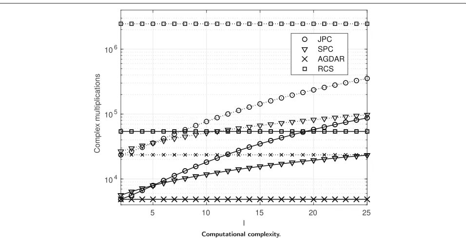
In Fig. 13, we compare the complexity of the various scenarios, by considering the number of complex multi-plications, as derived in Section4.4, as a function of the number of canceled pathsI. Parameters are those of Fig.3, so that we can compare the achieved MSE of the various schemes. We observe that the number of multiplications grows exponentially for the SPC and JPC techniques. We also report the number of complex multiplications for the
AGDAR and RCS methods that do not depend onI. We
note that the AGDAR has a remarkably lower complex-ity than other methods. However, we also notice that for M1 = 64 and M2 = 8, RCS has a significantly higher complexity with respect to the other methods. When comparing the MSE performance (Fig. 3), we see that AGDAR achieves a much lower MSE than SPC and JPC methods for a lower complexity (in terms of CMUX and CADD).
6 Conclusions
In this paper, we have proposed channel estimation tech-niques for mm-Wave massive MIMO systems, based on a CS approach, where we have exploited the sparse nature of the channel, considering in particular the small number of channel paths at those frequencies. Efficient innova-tive solutions based on the adapinnova-tive restart of the Nes-terov accelerated gradient algorithm have been explored. Numerical results have shown the superiority of the pro-posed approaches with respect to existing procedures, with similar or lower computational complexity. We have also considered the effects of sectorization and proposed a channel tracking technique that exploits slow channel variations.
Endnotes
1Note that other configurations (e.g., UPA on one side
and ULA on the other side) can be obtained with similar derivations.
Fig. 13Computational complexity. Average number of complex multiplications as function ofIfor various systems with (M1=32,M2=4) (solid lines) and (M1=64,M2=8) (dotted lines), ULA system with (Nr=32,Nt=4) and SNR of 10 dB
2In general, the number of symbols can be larges than
Ntbut we consider here this simpler case for the sake of conciseness.
Appendix A: CS channel estimation for UPA
For a UPA system, we denote asD2andD3the number of transmit antennas along they-andz-axes, respectively; therefore, Nt = D2× D3. Similarly D0 andD1 are the numbers of antennas at the receiver along the two axes; therefore,Nr=D0×D1. The channel matrix has entries
HUPA
i1+D1i0,i3+D3i2= L
l=1 αle2πη
l
0i0je2πηl1i1je2πη2li2je2πηl3i3j.
(30)
The channelHUPAis transformed into the channel col-umn vectorhUPA = vecHUPA ∈ CNrNt×1with entries
hUPA
i0+D0i1+D0D1i2+D2D1D0i3 =
HUPA
i1+D1i0,i3+D3i2.
(31)
We also define the 4D-DFT matrix as F4D ∈
CNrNt×(M0M1M2M3)with entries
F4D(i0+D0i1+D1D0i2+D2D1D0i3,f0+M0f1+M1M0f2+M2M1M0f3)
=
3
d=0 e−
2πidfdj
Md . (32)
Lastly, we define the column vector vUPA of length M0M1M2M3withLnon-zero entries, namely
vUPA
¯ l
0+M0¯l1+M1M0¯l2+M2M1M0¯l3
=αl (33)
where
¯
l
0=
ηl
0M0 ,¯l1=
ηl
1M1 ,¯l2=
ηl
3M3 ,¯l3=
ηl
3M3 .
(34)
From (30), we can approximate the channel as
hUPA≈F4DvUPA. (35)
Similarly, we can define hUPA and vUPA for the LS estimate of the channel and its dual representation. The AGDAR and RCS algorithms for UPA can be obtained as described in Section4, withF,h, andvreplaced byF4D,
hUPA, andvUPA, respectively.
Appendix B: On the choice ofMd
The choice of the number of DFT points per dimension Md is important to determine the performance of the channel estimation algorithm. From (34), we have that the AGDAR solution approximatesηldwith a quantized value taken overMdpossible points. Therefore, we can write the
quantization error on thel-th path as
l
d=ηld−
ηl dMd
Md
Focusing now on a scenario wherein ULAs are used at both transmitter and receiver, assuming that all other esti-mates (i.e., the amplitude angle estiesti-mates of each path) are correct and the only imperfection is the quantization error, from (36), the estimated channel can be written as (compared with (1)) of the channel estimate is
γ(q)= 1
Now, assuming that the amplitudes and angles are inde-pendent random variables, we have
γ(q)= 1
Let us assume that arrival and departure angles (ϑlrand
ϑt
l) are uniformly distributed in the interval [ 0, 2π)and
ηl
This MSE provides a guideline for the choice ofMd, as
we must have at leastγ(q)> σ2, so that quantization does not introduce more errors (in terms of its power) than noise already present.
Abbreviations
3GPP: Third-generation partnership project; AGDAR: Accelerated gradient descent with adaptive restart; AWGN: Additive white Gaussian noise; BPDN: Basis pursuit denoise; BS: Base station; CBP: Continuous basis pursuit; CS: Compressed sensing; DFT: Discrete Fourier transform; FISTA: Fast iterative shrinkage-thresholding algorithm; IDFT: Inverse discrete Fourier transform; InH: Indoor Hotspot; ISTA: Iterative shrinkage-thresholding algorithm; JPC: Joint peak cancelation; LASSO: Least absolute shrinkage and selection operator; LOS: Line-of-sight; LS: Least square; MIMO: Multiple-input-multiple-output; ML: Maximum likelihood; MSE: Mean square error; NLOS: Non-line-of-sight OMP: Orthogonal matching pursuit; RCS: Re-weighted compressed sensing; RF: Radio frequency; RMa: Rural macro cell; SNR: Signal to noise ratio; SPC: Single peak cancelation; SSAMP: Sparsity adaptive matching pursuit; UE: User equipment; ULA: Uniform linear array; UMa: Urban macro cell; UMi: Urban micro cell; UPA: Uniform planar array
Acknowledgements No acknowledgements.
Funding
This work has been supported by Huawei Technology, Italy.
Availability of data and materials No data is available.
Authors’ contributions
The ain contributions of this paper are as follows: The proposal of two new algorithms for the channel estimation in mm-wave systems and the performance evaluation of the proposed algorithms in a 5g scenario. All authors read and approved the final manuscript.
Competing interests
The authors declare that they have no competing interests.
Publisher’s Note
Springer Nature remains neutral with regard to jurisdictional claims in published maps and institutional affiliations.
Author details
1Department of Information Engineering, University of Padova, via Gradenigo
6/A, Padua, Italy.2Huawei Technologies Italia, Milan, Italy.3Consorzio
Nazionale Interuniversitario per le Telecomunicazioni, Padua, Italy.
Received: 1 August 2018 Accepted: 31 October 2018
References
1. T. S. Rappaport, J. N. Murdock, F. Gutierrez, State of the art in 60-ghz integrated circuits and systems for wireless communications. Proc. IEEE. 99(8), 1390–1436 (2011)
3. Tecnical report, 5G; study on channel model for frequencies from 0.5 to 100 GHz (3GPP TR 38.901 version 14.3.0 release 14) (2018)
4. R. W. Heath, N. González-Prelcic, S. Rangan, W. Roh, A. M. Sayeed, An overview of signal processing techniques for millimeter wave MIMO systems. IEEE J. Sel. Top. Sig. Proc.10(3), 436–453 (2016).https://doi.org/ 10.1109/JSTSP.2016.2523924
5. A. Alkhateeb, O. E. Ayach, G. Leus, R. W. Heath, Channel estimation and hybrid precoding for millimeter wave cellular systems. IEEE J. Sel. Top. Sig. Proc.8(5), 831–846 (2014).https://doi.org/10.1109/JSTSP.2014.2334278 6. S. Montagner, N. Benvenuto, S. Tomasin, inProc 2015 IEEE Int. Conf. on
Communication Workshop (ICCW). Taming the complexity of mm-wave massive MIMO systems: Efficient channel estimation and beamforming, (2015), pp. 1251–1256.https://doi.org/10.1109/ICCW.2015.7247349 7. D. De Donno, J. P. Beltrán, D. Giustiniano, J. Widmer, in2016 IEEE
International Conference on Communications Workshops (ICC), Kuala Lumpur. Hybrid analog-digital beam training for mmWave systems with low-resolution RF phase shifters, (2016), pp. 700–705.https://doi.org/10. 1109/ICCW.2016.7503869
8. J. Lee, G. T. Gil, Y. H. Lee, Channel estimation via orthogonal matching pursuit for hybrid MIMO systems in millimeter wave communications. IEEE Trans. Commun.64(6), 2370–2386 (2016).https://doi.org/10.1109/ TCOMM.2016.2557791
9. J. Palacios, D. De Donno, D. Giustiniano, J. Widmer, in2016 IEEE 27th Annual International Symposium on Personal, Indoor, and Mobile Radio Communications (PIMRC), Valencia. Speeding up mmWave beam training through low-complexity hybrid transceivers, (2016), pp. 1–7.https://doi. org/10.1109/PIMRC.2016.7794709
10. S. Sun, T. S. Rappaport, in2017 IEEE International Conference on
Communications Workshops (ICC Workshops), Paris. Millimeter Wave MIMO channel estimation based on adaptive compressed sensing, (2017), pp. 47–53.https://doi.org/10.1109/ICCW.2017.7962632
11. X. Li, J. Fang, H. Li, P. Wang, Millimeter wave channel estimation via exploiting joint sparse and low-rank structures. IEEE Trans. Wirel. Commun. 17(2), 1123–1133 (2018).https://doi.org/10.1109/TWC.2017.2776108 12. G. Destino, M. Juntti, S. Nagaraj, inProc 2015 IEEE Global Conference on
Signal and Information Processing (GlobalSIP). Leveraging sparsity into massive MIMO channel estimation with the adaptive-LASSO, (2015), pp. 166–170.https://doi.org/10.1109/GlobalSIP.2015.7418178
13. Z. Marzi, D. Ramasamy, U. Madhow, Compressive channel estimation and tracking for large arrays in mm-wave picocells. IEEE J. Sel. Top. Sig. Proc. 10(3), 514–527 (2016).https://doi.org/10.1109/JSTSP.2016.2520899 14. S. Malla, G. Abreu, inProc 2016 Int. Symposium on Wireless Comm. Systems
(ISWCS). Channel estimation in millimeter wave MIMO systems: Sparsity enhancement via reweighting, (2016), pp. 230–234.https://doi.org/10. 1109/ISWCS.2016.7600906
15. Z. Gao, L. Dai, Z. Wang, inProc 2016 IEEE Int. Conf. on Commun. (ICC). Channel estimation for mmwave massive MIMO based access and backhaul in ultra-dense network, (2016), pp. 1–6.https://doi.org/10.1109/ ICC.2016.7511578
16. M. Kokshoorn, H. Chen, Y. Li, B. Vucetic, Beam-on-graph: Simultaneous channel estimation for mmwave MIMO systems with multiple users. IEEE Trans. Commun.PP(99), 1–1 (2018).https://doi.org/10.1109/TCOMM. 2018.2791540
17. Y. Nesterov, Gradient methods for minimizing composite objective function. Math. Program. Ser. B.140, 125–161 (2007)
18. E. J. Candès, M. B. Wakin, S. P. Boyd, Enhancing sparsity by reweighted1
minimization. J. Fourier Anal. Appl.14(5), 877–905 (2008).https://doi.org/ 10.1007/s00041-008-9045-x
19. A. M. Sayeed, Deconstructing multiantenna fading channels. IEEE Trans. Sig. Process.50(10), 2563–2579 (2002).https://doi.org/10.1109/TSP.2002. 803324
20. J. Mo, P. Schniter, N. G. Prelcic, R. W. Heath, inProc 2014 48th Asilomar Conference on Signals, Systems and Computers. Channel estimation in millimeter wave MIMO systems with one-bit quantization, (2014), pp. 957–961.https://doi.org/10.1109/ACSSC.2014.7094595 21. C. A. Balanis,Antenna Theory: Analysis and Design. (Wiley-Interscience,
Hoboken, New Jersey, 2005)
22. Y. S. Cho, J. Kim, W. Y. Yang, C. G. Kang,MIMO-OFDM Wireless Communications with MATLAB. (Wiley, Hoboken, New Jersey, 2010)
23. E. Björnson, E. G. Larsson, T. L. Marzetta, Massive mimo: ten myths and one critical question. IEEE Commun. Mag.54(2), 114–123 (2016).https://doi. org/10.1109/MCOM.2016.7402270
24. D. Tse, P. Viswanath,Fundamentals of Wireless Communication. (Cambridge University Press, New York, 2005)
25. S. Boyd, L. Vandenberghe,Convex Optimization. (Cambridge university press, Cambridge, 2004)
26. M. A. T. Figueiredo, R. D. Nowak, S. J. Wright, Gradient projection for sparse reconstruction: Application to compressed sensing and other inverse problems. IEEE J. Sel. Top. Sig. Proc.1(4), 586–597 (2007).https://doi.org/ 10.1109/JSTSP.2007.910281
27. B. O’Donoghue, E. Candès, Adaptive restart for accelerated gradient schemes. Found. Comput. Math.15(3), 715–732 (2015).https://doi.org/ 10.1007/s10208-013-9150-3
28. N. Parikh, S. Boyd, Proximal algorithms. Found. Trends Optim.1(3), 127–239 (2014).https://doi.org/10.1561/2400000003
29. A. Chambolle, R. A. D. Vore, N.-Y. Lee, B. J. Lucier, Nonlinear wavelet image processing: variational problems, compression, and noise removal through wavelet shrinkage. IEEE Trans. Image Process.7(3), 319–335 (1998).https://doi.org/10.1109/83.661182