Trade-Growth Nexus in Developing and Developed Countries: An Application of Extreme Bounds Analysis

915 TRADE-GROWTH NEXUS IN DEVELOPING AND DEVELOPED COUNTRIES: AN APPLICATION OF EXTREME BOUNDS ANALYSIS

Mansour Zarra-Nezhad

Professor of Economics, Shahid Chamran University, Ahvaz, Iran

Fatimah Hosseinpour

Department of Economics, Faculty of Economics and Social Sciences, Shahid Chamran University, Ahvaz, Iran

Seyed Aziz Arman

Department of Economics, Faculty of Economics and Social Sciences, Shahid Chamran University, Ahvaz, Iran

ABSTRACT

In this study, we investigated the relationship between foreign trade and economic growth in the

developing and developed countries by using extreme bounds analysis approach. For this we used

unbalanced panel data of 103 variables of 94 countries (74 developing countries and 20 developed

countries) during 1990-2010. The estimation results of more than 1.6 million regressions show that

more foreign trade indices are robust determinants of economic growth and have robustly positive

effect on the economic growth of each country regardless of level of development. In the other

words, results of this study support views of free trade advocates.

Keywords:

1. INTRODUCTION

There are different and even inconsistent views about the relation between economic growth

and international trade in economic literature. Brilliant economists such as Hume, Smith, Ricardo,

Mill, Singer, Prebisch, Myrdal have different ideas about the relation between free trade and

economic growth. Theories about the impact of trade on economic growth could divide into two

different groups. The first are consistent with free trade. The idea is that international trade is an

engine of economic growth and accelerated it. The oldest view is Mercantilism’s. Advocates of this

doctrine believed that just positive trade balance cause economic growth. Smith (1776),Ricardo

(1817) presented absolute advantage and comparative advantage theories and pointed out that

Asian Economic and Financial Review

916 foreign trade increase production level and economic growth. John Stuart Mill believed that

international trade causes more efficiency of production factors that he named it direct advantage of

foreign trade. Heckscher, Ohlin and Samuelson likewise some other economists support free trade.

Endogenous theory of growth was considered trade policy and its rule on R & D activity.

International product cycle also has some implications for economic growth of both developed and

developing countries. As Shaw (1992) pointed out invention and new products take place in the

developed countries where R & D activity is well developed. After some time, technology transfers

to the less advanced country and they can produce these goods. Hence, trade in manufactured

products occurred on the basis of exchange between the newest innovative goods produced only in

the developed countries and the oldest goods that now produced predominantly by the developing

countries. Indeed the developed countries import the goods that initially they exported them.

According to this idea, international trade contributes in faster economic growth in both developed

and developing countries. In developed countries, process of the migration of production of old and

simple good to developing countries released resources for use R&D activity and produce of new

goods. In the developing countries also growth occurs faster, because the resources needed for

learning and adapting the techniques imported from the developing countries are less than those

needed for autonomous new product development. In both countries, the subsidization of learning

activities (innovation in developed countries, imitation in the developing) may be enhanced long

run growth rates. But against these ideas, some believed that trade decrease economic growth of

developing countries and increase international inequality. Among economist of this group, we can

refer to Myrdal (1957) and Singer (1982). They believed that just developed countries benefits

from international trade. In empirical aspect again, many studies have found a positive relation

between trade and economic growth (Balassa, 1985; Chow, 1987)),Krueger (1990), and Sengupta

and Espana (1994),Ekanayake (1999), Vamvakidis (1998)). Experiments of some countries, for

example East Asian countries, show that presence in global market and gain from foreign trade is

an important path for developing countries to improve their economies. In another hand, Krugman

(1994), Rodriguez and Rodrik (1999),Vamvakidis (2002), Madsen (2009) and Singh (2010) argue

that the effect of free trade on growth is questionable. Dowrick and Golley (2004) pointed out that

the impact of trade on growth varies in both sign and significance with change the level of

economic development.

As mentioned, there is consensus nor in theoretical views and not in empirical studies about

the effect of foreign trade on economic growth, special about developing countries. The reason of

difference in the results of empirical studies could be because of their specification of growth

regressions. Researchers know well that results of regressions are sensitive to change in

specification. For specification of empirical growth regressions, if we accept the variables that

introduced by theories and confirmed by empirical researches as determinants of growth,

multiplicity of theories and empirical studies cause to introduce large number of growth

determinants. For example, Durlauf et al. (2005) in their outstanding review introduced about 150

917 and its sign has been compatible with a growth theory. It is worthy to mention that economic

growth theories, as Brock and Durlauf (2001) mentioned, are open ended, in the sense that they are

compatible with each others. Hence, if there is a set of K theories that all of them are logically

compatible, there exist _- possible specifications of growth regressions that each regression is

based on a special combination of theories. Therefore selecting explanatory variables is often ad

hoc and the results are likely to be sensitive to the selected variables.

These issues along with measurement considerations persuaded economists to examine

variables between set of variables that are identified until now as determinants of growth, instead of

following solely theories. Many empirical studies tried to determine variables that influence

economic growth only using one or few regressions. Although the results of these studies might be

logical and compatible with the theories, but the results could differ when changing the

specification. Thus rely on these results might be diversionary. This weakness has been pointed

out, among others, by Leamer (1983) where he emphasized that under uncertainty of model

selection one must show how much the result depends on which variable are included in the

regression. Therefore one should subject regressions to change in specification. This sensitivity

analysis provides a convincing justification for removal or inclusion of individual variables in the

probably true regression. One of the best approaches for selecting main determinant among vast

potential determinants is extreme bounds analysis (EBA). This approach is attributed to Leamer

and Leonard (1983). Levine and Renelt (1992) applied Leamer’s extreme bounds test for the first

time to identify robust empirical relations discussed in the economic growth literature. Levine and

Zervos (1993) pointed out the EBA helps clarify the degree of confidence that can be placed to the

partial correlations between growth and individual variables. If an indicator is roboustly correlated

with long-run economic growth, then one should feel more confident about its association with

growth than an indicator that has a fragile link. Merikas et al. (2000) used extreme bound analysis

Levine and Renelt (1992) in the cross-countries framework (92 countries) to determine robustness

of relationship between 3 proxies of trade openness (average of export share of GDP, average rate

of export growth and the real exchange rate distortion) and economic growth. Their results show

positive and robust link between export share expansion and economic growth, and negative and

robust relation of the real exchange rate distortion and growth.

Hence, the purpose of this paper is to investigate the relationship between trade expansion and

economic growth and its robustness in the developed and developing countries to test two different

ideas about the effect of foreign trade on economic growth. Also this study for checking the

sensitivity of results to change in specification use extreme bounds analysis approaches of Levine

and Renelt (1992) and Sala-I-Martin (1997a). We implement these approaches with the unbalanced

panel data of 21 years to determine robustness of correlation of trade proxies on economic growth

in 74 developing countries and 20 developed countries. For checking the sensitivity of results to

change in specification we use 103 variables as potential determinants of growth. The paper is

918 presents the results from the extreme bounds analysis. Section four is allocated to concluding

remarks.

2. METHODOLOGY AND DATA

Leamer (1978) and Leamer (1983) suggested a solution for the problem of uncertainty in

model selection. They named it extreme bound analysis that essentially is an approach for reporting

sensitivity of result to variation in model specification. The EBA version of Levine and Renelt

(1992) employ a linear regression framework as follows:

(1)

where Y stands for growth rate of GDP per capita, I for a set of base variables always included in

the regression, M for a variable of interest (trade proxies) that we want to examine its fragility or

robustness and Z for a set of up to three variables that we choose from a set of variables that

identified as a potential determinants of economic growth.

The approach of the Levine and Renelt (1992) is as follows. First, one should choose the

variables were emphasized in previous empirical studies and then estimate a base regression that

includes only the I-variables and the variables of interest. Second, regressions including all possible

linear combinations of up to three Z-variables should be estimated to identify the highest and

lowest coefficient of the M-variable ( ). The extreme upper is defined as the maximum value of

, the lower bound as the minimum value of - , where is the estimated

coefficient of M-variable and is its standard deviation in jth model. If the extreme upper bound

and lower bound have same sign, then M-variable is referred to be robust, otherwise is fragile. As

(Sala-I-Martin, 1997b) pointed out one should note that “this amounts to say that if one finds a

single regression for which the sign of the coefficient change or becomes insignificant, then the

variables is not robust” (p. 178). In particular, if is consistently significant and of the same sign in all regressions, then the M-variable is robust; otherwise it is fragile.

Sala-I-Martin (1997b) criticized on Levine and Renelt approach and argued that their criteria

are very rigid and is really hard for any variable to pass it. He introduced the confidence level to

quit giving the label of one or zero to the variables, and considered the whole distribution of

coefficients of the M-variable, ( ). He computed the fraction of cumulative distribution function

lying on each side of zero and named the greatest area CDF(0). He also used the weighted approach

to give more importance to the regression that is more likely to be true. He used the goodness of fit

of model as a likelihood of being true. Sala-i-Martin pointed out even though each individual

follow a t student distribution, all estimates might be scattered in an unrecognized fashion. Hence,

one can operate under two different assumptions.

If the distribution of the estimates of s is normal, one can calculate a cumulative distribution

function (CDF) from the mean and the standard deviation of the distribution. The likelihood L for

each possible model based on goodness of fit is necessary to calculate weighted mean of and

919

̂ ∑ (2)

̂ ∑ (3)

⁄∑ (4)

where stands for likelihood of jth regression. If the distribution of the estimates of

across all models is not normal, one can compute individual CDF(0) for each regression, , then

compute the aggregate CDF(0) of as the weighted mean of all the individual CDF(0) that the

weights are similar to normal case (equation(4)).Variables that their CDF are larger than 0.95 are

labeled robust.

For more details suppose one wants to examine robustness of potential determinants of growth,

for example growth of export, within a set of 103 variables. Four variables leaved as I-variables,

one variable is the interested (growth of export) that is examined whether it significantly and

robustly affects economic growth and rest of them, 98 variables counted as Z-variables that allow

to combine in subset of up to three. Based on combination formula ( ( ) ( - ) ⁄ that

i=1,2,3) one have 98 single, 4753 binary, 152096 ternary combinations. So 156947 regressions, in

addition to a base regression are estimated. In Levin and Renelt procedure if all 156948 coefficients

of interest variable were statistically significant and of the same sign, it called robust determinant

of growth, otherwise it is fragile.

The rule of decision in Sala-i-Martin approach is different. In his procedure, one must consider

the distribution of estimated coefficients. Under normal assumption and by computing ̂ and ̂

(equation 2 and 3), one can standardize the distribution of estimated coefficients then based on

normal standard distribution table compute CDF(0). It should be noted that area under density

function divided into two areas by zero, the greater area regardless of whether it is below or above

zero, called CDF(0). But under non-normal assumption according to that we know each estimated

variables have t-student distribution and this distribution tend to normal distribution if observation

number is considerable, and under the assumption that ( ̂ ) one can standardize estimated

coefficients then based on normal standard distribution table compute individual CDF(0) for each

regression, then as we pointed above, compute the aggregate CDF(0) of as the weighted mean

of all the individual CDF(0). Therefore if aggregate CDF(0)>0.95, variable is significantly and

robustly correlated with growth rate. As Sala-I-Martin (1997b) pointed out if for variable 1,

CDF(0)=0.95 and for variable 2, CDF(0)=0.52, then variable 1 is more likely to be robustly

correlated with economic growth.

It is important to know that Levine and Renelt (1992) and Sala-I-Martin (1997a) and other

brilliant empirical researches (for example, Levine and Zervos (1993), (Hoover and Perez, 2004)

estimated their models with cross-section data. There is few work that use panel data with EBA in

economic growth literature, of which we can refer to Rao and Cooray (2010)who used panel data

for only 13 variables and 7 countries of South Asia and to Chain and lee (1999) who used panel

920 In this study, we apply EBA on 103 variables using random-effects model to estimate the

following equation:

(5)

Where terms are the random effects for country i. The random-effects model was used because

when some variables are constant for each individual, fixed-effects regression is not an effective

tool due to that such variables cannot be included (Dougherty, 2007). The panel data of the study is

composed of 74 developing countries and 20 developed countries over the period 1990-2010. The

countries are listed in table (1) and (2), respectively.

Levine and Renelt (1992) and Sala-I-Martin (1997b) used respectively 57 and 63 variables

which found to be statistically significant in the previous studies. Durlauf et al. (2005) also

collected 145 variables as the potential determinants of growth that at least were statistically

significant in one study.

As regard to the variables, it should be noted that we could collect data on 103 variables

considered as potential determinants of economic growth in the literature for the selected countries.

Most of Levine and Renelt, and Sala-i-Martin variables are included in the present study. The

dependent variable is growth rate of per capita GDP. The I-variables were chosen following the

Levine and Renelt (1992). The I-variables are composed of investment share of GDP (IR), the

initial level of real GDP per capita in 1990 (IN), the secondary school enrollment rate (ENSE) and

annual rate of population growth (POPG). These variables, as Levine and Renelt (1992) also

pointed out, have been selected on the base of large range of previous empirical studies and

economic theories that rely on constant returns to reproducible factors and endogenous

technological change. These I-variables are compatible with new economic growth (endogenous

growth theories). As Mankiw et al. (1992)mentioned, the I-variables are entered on the basis of

human capital-augmented neoclassical growth model. Barro (2003) for inclusion of investment

ratio pointed out that the effect of the saving rate in the neoclassical growth model is measured

empirically by investment ratio. The M variables are:

1. The export share of GDP (EXGDP)

2. The import share of GDP (IMGDP)

3. Fraction of primary products in total exports (PRIEX)

4. Growth of export share of GDP (GEXGDP)

5. Export growth (GEX)

6. Import growth (GIM)

7. Machinery and equipment imports (MACHIN)

8. Oil export (OILEX)

9. Trade share of GDP (OPEN)

921 The Z variables (89 rested variables) and their sources are described in detail in appendix A.

Like Levine and Renelt (1992) and Levine and Zervos (1993), when evaluating the robustness of

each M variable, we restrict this pool of Z-variables by excluding any variable which may measure

the same phenomenon.

3. RESULTS

The results Levine and Renelt approach for developing and developed countries are presented

respectively in table (3) and (5). The column (I) in these tables presents lowest and highest as well

as coefficient of base regression for each variable. The column (II) reports the t statistics and

column (III) reports p values. The column (IV) present the fraction of significant coefficients

divided to negative and positive. The columns (V) and (VI) respectively report fractions of positive

and negative coefficient from all coefficients (significant or insignificant). In the tables (4) and (6),

Sala-i-Martin approach results for both groups of countries are reported. The columns (I) and (II)

report the weighted mean of estimated coefficients of M-variables and weighted standard errors,

respectively. The columns (III), (IV) and (V) present the significant level or CDF(0) in weighted

normal, weighted non-normal and unweighted non-normal cases, respectively. The column (VI)

present result of skewness and kurtosis test for normality of coefficients. At the end in both

procedures, last column report status of robustness. As mentioned before, in Levine and Renelt

approach if is consistently significant and of the same sign in all regressions, then the

M-variable is robust; otherwise it is fragile. Also in Sala-i-Martin approach, if CDF(0) is more than

0.95, the variable is robust.

Results of regressions in developing countries show that growth of export share of GDP

(GEXGDP), export growth (GEX), import growth (GIM) and Growth of trade share of GDP

(OPENG) passed too strong test of Levine and Renelt and coefficients of these variables are

significant in all regressions, so introduced as robust determinants of growth. Although export

share of GDP (EXGDP) and Oil export (OILEX) could not earn robust label, they were found

significant respectively in 99.94 and 99.31 percent of specifications. The coefficients of machinery

and equipment imports (MACHIN) and fraction of primary products in total exports (PRIEX) were

positive and significant in more than half of regressions.

Results of Sala-i-Martin approach for developing countries in table (4) show that in addition to

4 robust determinants in Levine and Renelt procedure, three variables of export share of

GDP(EXGDP), fraction of primary products in total exports (PRIEX) and Oil export (OILEX) have

labeled as robust. The CDF(0) value for all of these three variables in three cases of normality and

weights, are more than 0.95. Judgment pertaining to machinery and equipment imports (MACHIN)

needs more considerations. According to the result of skewness and kurtosis test for normality,

coefficients distribution of MACHIN is non-normal. So the CDF(0) values in weighted an

unweighted non- normal cases are the judging criteria. CDF(0) in unweighted non- normal case is

less than 0.95 and in weighted non- normal case is more than 0.95, hence given at Sala-i-Martin

922 in this approach are fragile, too. The results indeed confirm positive effects of trade openness on

economic growth in developing countries.

Results of Levine and Renelt approach in developed countries show that just import growth

(GIM) and Growth of trade share of GDP (OPENG) passed too strong test of Levine and Renelt

and coefficients of these variables are significant in all regressions, so introduced as robust

determinants of growth, as observed in table (5). Although in developed countries growth of export

share of GDP (GEXGDP), export growth (GEX), export share of GDP (EXGDP), import share of

GDP (IMGDP) and fraction of primary products in total exports (PRIEX) could not receive robust

label but their coefficients were significant and positive respectively in 99.3, 99.92, 93.71, 92 and

86.76 percent of regressions. Results of Sala-i-Martin approach for developed countries in table (6)

show that for these countries 7 out of 10 indices are robust that in two cases are common with

results of Levine and Renelt approach. With judging procedure of Sala-i-Martin, growth of export

share of GDP (GEXGDP), export growth (GEX), export share of GDP (EXGDP), import share of

GDP (IMGDP) and fraction of primary products in total exports (PRIEX) are added to robust

determinants that identified in Levine and Renelt approach.

It is worth noting that export measurements in developing countries are more robust than

developed countries. In the developing countries 4 variables could past very rigid and strict test of

Levine and Renelt but in developed countries just two variables could pass this test. One of the 7

robust variables is different in two groups of countries. In the developing countries value of oil

exports is robust but in developed countries is not, also import share of GDP in developed countries

is robust but in developing countries is not. We totally estimate 1.6 million regressions that show

most of trade measurement in all countries, developing and developed, are robust determinants of

economic growth and enhance it.

4. CONCLUDING REMARK

Our empirical investigation between growth and trade measures has provided evidence that in

a large sample of developing and developed countries, higher rates of economic growth are

robustly correlated with higher rates of trade. So it seems that abroad-based economic growth is

essential to sustainable, long-term growth. 7 out of 10 indices of free trade in these countries are

robust determinants of economic growth. These variables, regardless of their level of development

have positive effect on economic growth of both groups of countries. Hence, these findings confirm

views that support free trade and are opposite with Myrdal idea, so policymakers of developing

countries should pay attention more in this part of economics.

REFERENCES

Balassa, B., 1985. Exports, policy choices, and economic growth in developing countries after the 1973 oil shock. Journal of Development Economics, 18(1): 23-35.

923 Brock, W. and S. Durlauf, 2001. Growth empirics and reality. World Bank Economic Review, 15(2): 229–

272.

Chain, W.M. and K.J. lee, 1999. Economic growth regressions for the American states: A sensitivity analysis. Economic Inquiry, 37(2): 242-257.

Chow, P.C.Y., 1987. Causality between export growth and industrial performance: Empirical evidence from the NICs. Journal of Development Economics, 23(1): 53-63.

Dougherty, C., 2007. Introduction to econometrics. 3rd Edn., Oxford University Press.

Dowrick, S. and J. Golley, 2004. Trade openness and growth: Who benefits? Oxford Review of Economic Policy, 20(1): 38-56.

Durlauf, S.N., P.A. Johnson and J.R.W. Temple, 2005. Growth econometrics, handbook of economic growth, chapter 8. Amsterdam: North-Holand. pp: 555-677.

Ekanayake, E.M., 1999. Exports and economic growth in Asian developing countries: Cointegration and error correction models. Journal of Economic Development, 24(2): 43-56.

Hoover, K.D. and S.J. Perez, 2004. Truth and robustness in cross-country growth. Oxford Bulletin of Economics and Statistics, 66(5): 765-798.

Krueger, A.O., 1990. Trends in trade policies of developing countries, In Charles S. Pearson and James Riedel, eds., The direction of trade policy. Cambridge, MA: Blackwell. pp: 87-107.

Krugman, P., 1994. The myth of Asia’s miracle, foreign affairs, 73(6): 62-78.

Leamer, E., 1978. Specification searches. New York: Wiley.

Leamer, E., 1983. Let’s take the con out of econometrics. American Economic Review, 73(1): 31–43.

Leamer, E. and H. Leonard, 1983. Reporting the fragility of regression estimates. Review of Economics and Statistics, 65(2): 306–317.

Levine, R. and D. Renelt, 1992. A sensitivity analysis of cross-country growth regressions. American Economic Review, 82(4): 942–963.

Levine, R. and S. Zervos, 1993. What we have learned about policy and growth from cross-country regressions. American Economic Review, 83(2): 426–430.

Madsen, J.B., 2009. Trade barriers, openness, and economic growth. Southern Economic Journal, 76(2): 397-418.

Mankiw, N.G., D. Romer and D.N. Weil, 1992. A contribution to the empirics of economic growth. Quarterly Journal of Economics, 107(2): 407–437.

Merikas, A., G.S. Vozikis and A. Merikas, 2000. Trade openness and economic growth revisited. The Journal of Applied Business Research, 16(3): 75-86.

Myrdal, G., 1957. Economic theory and underdeveloped regions. London: Duckworth.

Rao, B.B. and A. Cooray, 2010. Determinants of the long-run growth rate in the South-Asian countries. University Library of Munich, Germany, MPRA Paper No. 26493.

Ricardo, D., 1817. On the principles of political economy and taxation. Cambridge: Cambridge University Press, [1951].

Rodriguez, F. and D. Rodrik, 1999. Trade policy and economic growth: A skeptic’s guide to the cross-national

924 Sala-I-Martin, X., 1997a. I just ran 4 million regressions. National Bureau of Economic Research Working

Paper No. 6252.

Sala-I-Martin, X., 1997b. I just ran 2 million regressions. American Economic Review, 87(2): 178–183. Sengupta, J.K. and R. Espana, 1994. Exports and economic growth in Asian NICs: An econometric analysis

for Korea. Applied Economics, 26(1): 45-51.

Shaw, G.K., 1992. Policy implications of endogenous growth theory. Economic Journal, 102(412): 611–621. Singer, H.W., 1982. Terms of trade controversy and evolution of soft financing: Early years in the U.N.:

1947-51. IDS Discussion Paper, No. DP181, November, Sussex.

Singh, T., 2010. Does international trade cause economic growth? A survey. The World Economy, 33(11): 1517- 1564.

Smith, A., 1776. An Inquiry into the nature and causes of the wealth of nations. New York: Random House, [1937].

Vamvakidis, A., 1998. Regional integration and economic growth. The World Bank Economic Review, 12(2): 251-270.

Vamvakidis, A., 2002. How robust is the growth-openness connection? Historical evidence. Journal of Economic Growth, 7(1): 57-80.

Table-1. Developing countries names

Algeria Albania Kuwait United Arab Emirates

Argentina Latvia Oman Tanzania

Bangladesh Madagascar Gabon Thailand

Armenia Malawi Gambia, The Yemen, Rep

Bolivia Malaysia Guyana Ukraine

Botswana Mali Guatemala Tunisia

Brazil Moldova Honduras Turkey

Ethiopia Mongolia Qatar Uganda

Belarus Mexico India Uruguay

Cameroon Morocco Indonesia Venezuela

Bahrain Mozambique Iran Vietnam

Bulgaria Namibia Jordan Zimbabwe

Chile Nicaragua Kenya Romania

China Niger Russia Senegal

Colombia Nigeria Saudi Arabia Lithuania

Lebanon Pakistan Sudan Philippines

Ecuador Panama South Africa

Egypt Paraguay Sri Lanka

925 Table- 2. Developed countries names

Australia France Japan Spain

Austria Germany Netherlands Sweden

Canada Greece New Zealand Switzerland

Denmark Ireland Norway United Kingdom

Finland Italy Portugal United States

926 Table-4. Results of Sala-i-Martin approach in developing countries

927 Table- 6. Results of Sala-i-Martin approach in developed countries

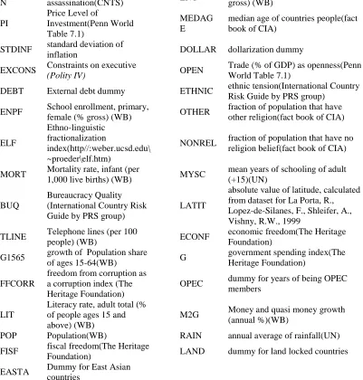
Appendix A

variable description variable description

EXGDPG growth of Fraction of export

in GDP(WTO) CREDVA variability of credit growth

EXG export growth(WTO) INVSTF investment freedom(The Heritage

Foundation)

IMG import growth (WTO) ENSF School enrollment, secondary,

female (% gross)

BM Broad money (% of

GDP)(WB) RELF religion fractionalization

INF inflation growth(WB) FERT Fertility rate(births per

woman)(WB)

CREDV O

volatility of domestic credit to private sector as a % gdp(WB)

BUD fraction of population that are buddhist

DEF deficit % of GDP (WEO

database of IMF) BRIT british colony dummy

HE Health expenditure, public

(% of GDP)(WB) SUR

survival rate of adult to age 60(per 1000)

PRIEX Fraction of primary products

in total exports(WTO) BUSSF

business freedom(The Heritage Foundation)

OPENG

Trade (% of GDP) growth as openness growth (Penn World Table 7.1)

CHRIS fraction of population that are chiristian(fact book of CIA)

IMG Fraction of import in

GDP(WTO) LDI

Linguistic diversity

index(www.ethnologue.com)

MSH

money shock, volatility component of m1(money supply)(WB)

MUS fraction of population that are muslim(fact book of CIA)

ENPM School enrollment, primary,

male (% gross)(WB) PRIGHT

property rights(The Heritage Foundation)

CORR

corruption

index(International Country Risk Guide by PRS group)

FINF financial freedom(The Heritage Foundation)

928 Heritage Foundation)

MING fraction of mining in

GDP(UN) LATIN Latin America dummy

GSTAB

Government

Stability(International Country Risk Guide by PRS group)

RULE rule of law (International Country Risk Guide by PRS group)

TRF trade freedom(The Heritage

Foundation) ARLAND Arable land (% of land area)(WB)

IR Investment Share of

GDP(Penn World Table 7.1) ENSM

School enrollment, secondary, male (% gross)(WB)

VOICE

Voice and Democratic Accountability

(International Country Risk Guide by PRS group)

GENDER

gender equality as a social development

index(http://www.indsocdev.org)

GIN

standard deviation of GDP growth as growth innovation (WB)

HINDU fraction of population that are hindu

URB Urban population (% of

total)(WB) ENSE

School enrollment, secondary (% gross)(WB)

POPG Population growth PC Price Level of Consumption(Penn

World Table 7.1)

WAR

dummy for war and duration(www.war-memorial.net)

GGC

growth of Government

Consumption Share of GDP (Penn World Table 7.1)

LPRATE

Labor participation rate, total (% of total population ages 15+)(WB)

AREA Surface area (sq. km)(WB)

STDMSH standard deviation of money

shock LTOTAL total Labor force,(WB)

ENP School enrollment, primary

(gross)(WB) MILIT military expenditure %GDP(WB)

SAFRIC Sub-Saharan Africa dummy DENS Population density (WB)

EXG Fraction of export in GDP CIVIC

civic activism as a social development

index(http://www.indsocdev.org)

IN

GDP per capita in 1990 as initial income GDP (Penn World Table 7.1)

DEM

democratic countries

dummy(Torsten Persson and Guido Tabellini :2009)

LIFE Life expectancy at

birth,(years) (WB) INF

Inflation, GDP deflator (annual %)(WB)

FDI

Foreign direct investment, net inflows (% of GDP) (WB)

65AB Population ages 65 and above (% of total) (WB)

GC

Government Consumption Share of GDP (Penn World Table 7.1)

COAST Coastline (fact book of CIA)

BMI black market exchange rate

primum index(FEW) REVCO revolution and coup detat(CNTS)

CREDG

growth of domestic credit to private sector as a % GDP(WB)

POP14 Population ages 0-14 (% of total)(WB)

OIL

Value of oil exports U.S. dollars(billion)(WEO database of IMF)

929 ASSASI

N

number of political

assassination(CNTS) ENT

School enrollment, tertiary (% gross) (WB)

PI

Price Level of

Investment(Penn World Table 7.1)

MEDAG E

median age of countries people(fact book of CIA)

STDINF standard deviation of

inflation DOLLAR dollarization dummy

EXCONS Constraints on executive

(Polity IV) OPEN

Trade (% of GDP) as openness(Penn World Table 7.1)

DEBT External debt dummy ETHNIC ethnic tension(International Country

Risk Guide by PRS group)

ENPF School enrollment, primary,

female (% gross) (WB) OTHER

fraction of population that have other religion(fact book of CIA)

ELF

Ethno-linguistic fractionalization

index(http//:weber.ucsd.edu\ ~proeder\elf.htm)

NONREL fraction of population that have no religion belief(fact book of CIA)

MORT Mortality rate, infant (per

1,000 live births) (WB) MYSC

mean years of schooling of adult (+15)(UN)

BUQ

Bureaucracy Quality (International Country Risk Guide by PRS group)

LATIT

absolute value of latitude, calculated from dataset for La Porta, R., Lopez-de-Silanes, F., Shleifer, A., Vishny, R.W., 1999

TLINE Telephone lines (per 100

people) (WB) ECONF

economic freedom(The Heritage Foundation)

G1565 growth of Population share

of ages 15-64(WB) G

government spending index(The Heritage Foundation)

FFCORR

freedom from corruption as a corruption index (The Heritage Foundation)

OPEC dummy for years of being OPEC

members

LIT

Literacy rate, adult total (% of people ages 15 and above) (WB)

M2G Money and quasi money growth

(annual %)(WB)

POP Population(WB) RAIN annual average of rainfall(UN)

FISF fiscal freedom(The Heritage

Foundation) LAND dummy for land locked countries

EASTA Dummy for East Asian

countries