A third order Newton-like Method and its
applications
D. R. Sahu
∗a, R. P. Agarwal
†b, Y. J. Cho
‡c,dand V. K. Singh
§aa Department of Mathematics, Banaras Hindu University,
Varanasi-221005, India
bDepartment of Mathematics, Texas A&M University-Kingsville,
Kingsville, Texas 78363-8202, USA
cSchool of Mathematical Sciences,
University of Electronic Science and Technology of China, Chengdu, Sichuan, 611731, P. R. China
dDepartment of Mathematics Education,
Gyeongsang National University, Jinju 660–701, Korea
October 8, 2018
Abstract
In this paper, we study the third order semilocal convergence of the Newton-like method for finding the approximate solution of nonlinear operator equations in the setting of Banach spaces. First, we discuss the convergence analysis under ω-continuity condition, which is weaker than the Lipschitz and H¨older continuity conditions. Second, we apply our approach to solve Fredholm integral equations, where the first derivative of involved operator not necessarily satisfy the H¨older and Lipschitz continuity conditions. Finally, we also prove that the R-order of the method is 2p+ 1 for anyp∈(0,1].
Keywords: Nonlinear operator equations, Fr´echet derivative,ω-continuity condition, the Newton like method, Fr´edholm integral equation.
1
Introduction
Our main purpose of this paper is to compute solution of nonlinear operator equation of the form
F(x) = 0, (1.1)
where F :D⊂ X →Y is a nonlinear operator defined on an open convex subset D of a Banach spaceX with values into a Banach space Y.
A lot of challenging problems in physics, numerical analysis, engineering and applied mathematics are formulated in terms of finding roots of the equation of the form (1.1). In order to solve such problems, we often use iterative methods. There are many iterative methods available in literature. One of the central method for solving such problems is the Newton method [5, 6] defined by
xn+1 =xn−Fx′−n1F(xn) (1.2)
for each n≥0, where Fx′ denotes the Fr´echet derivative of F at point x∈D.
The Newton method and the Newton-like methods are attractive because it converges rapidly from any sufficient initial guess. A number of researchers [7, 10–25] have general-ized and established local as well as semilocal convergence analysis of the Newton method (1.2) under the following conditions:
(a) Lipschitz condition: ∥Fx′ −Fy′∥ ≤K∥x−y∥ for all x, y ∈D and for some K >0; (b) H¨older Lipschitz condition: ∥Fx′ −Fy′∥ ≤ K∥x−y∥p for all x, y ∈ D and for some
p∈(0,1] andK >0;
(c) ω-continuity condition: ∥Fx′ − Fy′∥ ≤ ω(∥x −y∥) for all x, y ∈ D and for some function ω :R+→R+.
On the other hand, many mathematical problems such as differential equations, inte-gral equations, economics theory, game theory and variational inequalities can be formu-lated into the fixed point problem [3, 30]:
for each n ≥ 0. The Banach contraction principle (see [3–5, 30]) provides sufficient con-ditions for the convergence of the iterative method (1.4) to the fixed point of G. More details for approximation of fixed points of nonlinear operators can be found in [31,33,34]. The Newton method and its variant [8,9] are also used to solve the fixed point problem of the form:
(I−G)(x) = 0, (1.5) where I is the identity operator defined on X and G : D ⊂ X → X is a nonlinear Fr´echet differentiable operator defined on an open convex subsetD of a Banach spaceX. For finding approximate solution of the equation (1.5), Bartle [28] used the Newton-like iterative method of the form
xn+1 =xn−(I −G′yn)
−1
(I−G(xn)) (1.6)
for each n ≥ 0, where G′x is Fr´echet derivative of G at point x ∈ D and {yn} is the
sequence of arbitrary points in D which are sufficiently closed to the desired solution of the equation (1.5). Bartle [28] has discussed the convergence analysis of the form (1.6) under the assumption that G is Fr´echet differentiable at least at desired points and a modulus of continuity is known forG′ as a function of x. The Newton method (1.2) and the modified Newton method are the special cases of the form (1.6).
Following the idea of Bartle [28], Rall [29] introduced the following Stirling’s method for finding a solution of the fixed point problem (1.5):
{
yn=G(xn),
xn+1 =xn−(I−G′yn)
−1(x
n−G(xn))
(1.7)
for each n≥0.
Recently, Parhi and Gupta [1, 2] have discussed the semilocal convergence analysis of the following Stirling-like iterative method for computing a solution of the equation (1.5):
zn=G(xn),
yn =xn−(I−G′zn)
−1(x
n−G(xn)),
xn+1 =yn−(I−G′zn)
−1(y
n−G(yn))
(1.8)
for each n≥0.
the sense of Parhi and Gupta [1, 2] is weaker than the H¨older and Lipschitz continuity conditions. Our iterative method covers a wide variety of iterative methods and so our results generalize the results of Parhi and Gupta [1, 2]. Finally, we apply our approach to solve the Fredholm integral equation, where the first derivative of involved operator not necessarily satisfy the H¨older and Lipschitz continuity conditions.
2
Preliminary
In this section, we discuss some technical results. Throughout the paper, we denote
B(X, Y) a collection of bounded linear operators from a Banach space X into a Banach spaceY andB(X) = B(X, X). For somer > 0,Br[x] andBr(x) are the closed and open
balls with center x and radius r, respectively, N0 =N∪ {0} and Φ denote the collection of nonnegative, nondecreasing, continuous real valued functions defined on [0,∞).
Lemma 2.1 (Rall [26], Page 50) Let L be a bounded linear operator on a Banach space
X. Then L−1 exists if and only if there is a bounded linear operator M in X such that
M−1 exists and
∥M − L∥ < 1 ∥M−1∥.
If L−1 exists, then
L−1≤ ∥M−1∥
1− ∥1−M−1L∥ ≤
∥M−1∥
1− ∥M−1∥ ∥M− L∥.
Lemma 2.2 Let0< k≤ 13 be a real number. Assume thatq = p+11 +kp for anyp∈(0,1] and the scalar equation
(1−kp(1 +qt)pt)p+1−
( qptp
p+ 1 +k
p
)p
qpt2p = 0
has a minimum positive rootα. Then we have the following:
(1) q > k for all p∈(0,1].
for all p∈(0,1] and 0< k ≤ 13. (2) Set
g(t) = (1−kp(1 +qt)pt)p+1−
( qptp p+ 1 +k
p
)p
qpt2p. (2.1) It is clear from the definition of g(t) that g(0) > 0, g(1) < 0 and g′(t) < 0 in (0,1). Therefore,g(t) is decreasing in (0,1) and hence the equation (2.1) has a minimum positive rootα∈(0,1). This completes the proof.
Lemma 2.3 Let b0 ∈ (0, α) be a number such that kp(1 +qb0)pb0 <1, where k, p, α and
q are same as in Lemma 2.2. Define the real sequences {bn}, {θn} and {γn} by
bn+1 =
(
qpbp n p+1 +k
p)pqpb2p n
(1−kp(1 +qb n)pbn)
p+1bn, (2.2)
θn=
(
qpbpn p+1 +k
p)qb2
n
1−kp(1 +qb n)pbn
, γn =
1 1−kp(1 +qb
n)pbn
(2.3)
for each n ∈N0. Then we have the following:
(1)
(
qpbp0 p+1+k
p
)p qpb2p
0 (1−kp(1+qb
0)pb0)p+1 <1.
(2) The sequence {bn} is decreasing, that is bn+1 ≤bn for all n∈N0. (3) kp(1 +qb
n)pbn <1 for all n∈N0. (4) bn+1 ≤ξ(2p+1)
n
bn for all n∈N0.
(5) θn≤ξ
(2p+1)n−1
p θ for all n ∈N
0, where θ0 =θ and ξ =γ0θp.
Proof. (1) Since the scalar equationg(t) = 0 defined by (2.1) has a minimum positive root α ∈ (0,1) and g(t) is decreasing in (0,1) with g(0) > 0 and g(1) < 0. Therefore,
g(t)>0 in the interval (0, α) and hence
(
qpbp
0
p+1 +k
p)pqpb2p
0
(1−kp(1 +qb0)pb0)p+1 <1.
(2) From (1) and (2.2), we have b1 ≤ b0. This shows that (2) is true for n = 0. Let
(2.2), we have
bj+2 =
(qpbp j+1
p+1 +k
p)pqpb2p j+1
(1−kp(1 +qb
j+1)pbj+1)
p+1bj+1 ≤
(qpbp j p+1 +k
p)pqpb2p j
(1−kp(1 +qb j)pbn)
p+1bj =bj+1. Thus (2) holds forn =j + 1. Therefore, by induction, (2) holds for all n∈N0.
(3) Since bn< bn−1 for each n= 1,2,3,· · · and kp(1 +qb0)pb0 <1 for all p∈(0,1], it follows that
kp(1 +qbn)pbn < kp(1 +qb0)pb0 <1.
(4) From (3), one can easily prove that the sequences{γn}and {θn} are well defined.
Using (2.2) and (2.3), one can easily observe that
bn+1 =γnθnpbn (2.4)
for each n∈N0. Put n = 0 andn = 1 in (2.4), we have
b1 =γ0θpb0 =ξ(2p+1) 0
b0
and
b2 =
(
qpbp1
p+1 +k
p)pqpb2p
1
(1−kp(1 +qb
1)pb1)
p+1b1
≤ (
qpbp
0
p+1 +k
p)pqp(ξb
0)2p (1−kp(1 +qb
0)pb0)p+1
b1
≤ ξ2p (
qpbp
0
p+1 +k
p)pqpb2p
0
(1−kp(1 +qb
0)pb0)p+1
b1
Hence (4) holds forn= 0 and n= 1. Letj >1 be a fixed integer. Assume that (4) holds for each n= 0,1,2· · · , j. From (2.3) and (2.4), we have
bj+2 =
(qpbp j+1
p+1 +k
p)pqpb2p j+1
(1−kp(1 +qb
j+1)pbj+1)p+1
bj+1
≤
(qpbp j+1
p+1 +k
p)pqp(ξ(2p+1)jb
j)2p
(1−kp(1 +qb
j+1)pbj+1)p+1
bj+1
≤ (ξ2p(2p+1)j)
(qpbp j p+1 +k
p)pqpb2p j
(1−kp(1 +qb
j)pbj)p+1
bj+1
≤ ξ2p(2p+1)jξ2p(2p+1)j−1· · ·ξ2p(2p+1)ξ(2p+1)bj+1 = ξ(2p+1)j+1bj+1.
Thus (4) holds forn =j + 1. Therefore, by induction, (4) holds for all n∈N0. (5) From (2.3) and (4), one can easily observe that
θ1 =
(
qpbp
1
p+1 +k
p)qb2 1
1−kp(1 +qb
1)pb1
≤ (
qpbp
0
p+1 +k
p)q(ξb
0)2 1−kp(1 +qb
0)pb0
≤ξ(2p+1)1p −1θ.
Hence (5) holds for n = 1. Let j >1 be a fixed integer. Assume that (5) holds for each
n= 0,1,2· · · , j. From (2.3), we have
θj+1 =
(qpbp j+1
p+1 +k
p)qb2
j+1
1−kp(1 +qb
j+1)pbj+1
≤ (
qpbp
0
p+1 +k
p)q
( ξ(2p+1)
j+1−1 2p b
0
)2
1−kp(1 +qb0)pb
0
= ξ(2p+1)
j+1−1
p θ.
3
Computation of a solution of the operator equation
(1.1)
Let X and Y be Banach spaces and D be a nonempty open convex subset of X. Let
F : D ⊂ X → Y be a nonlinear operator such that F is Fr´echet differentiable at each point of D and let L∈ B(Y, X) such that (I−LF)(D)⊆D. Starting with x0 ∈D and afterxn∈D is defined, we define the next iterate xn+1 as follows:
zn = (I−LF)(xn),
yn= (I −Fz′−n1F)(xn),
xn+1 = (I−Fz′−n1F)(yn)
(3.1)
for each n∈N0.
If we take X = Y, F = I−G and L =I ∈B(X) in (3.1), then the iteration process (3.1) reduces to the Stirling-like iteration process (1.8).
Before proving the main results, we establish the following:
Proposition 3.1 LetDbe a nonempty open convex subset of a Banach spaceX,F :D⊂ X → Y be a Fr´echet differentiable at each point of D with values in a Banach space Y
andL∈B(Y, X)such that(I−LF)(D)⊆D. Letω : [0,∞)→[0,∞) be a nondecreasing and continuous real-valued function. Assume that F satisfies the following conditions:
(1) ∥Fx′ −Fy′∥ ≤ω(∥x−y∥) for all x, y ∈D;
(2) ∥I −LFx′∥ ≤cfor all x∈D and for some c∈(0,∞). Define a mapping T :D→D by
T(x) = (I−LF)(x) (3.2)
for all x∈D. Then
∥I−FT x′−1FT y′ ∥ ≤ ∥FT x′−1∥ω(c∥x−y∥)
Proof. For any x, y ∈D, we have
∥I−FT x′−1FT y′ ∥ ≤ ∥FT x′−1∥∥FT x′ −FT y′ ∥ ≤ ∥FT x′−1∥ω(∥T x−T y∥)
= ∥FT x′−1∥ω(∥x−y−L(F(x)−F(y))∥) = ∥FT x′−1∥ω
(
∥x−y−L ∫ 1
0
Fy′+t(x−y)(x−y)dt∥ )
≤ ∥FT x′−1∥ω
(∫ 1
0
∥I−LFy′+t(x−y)∥dt∥x−y∥ )
≤ ∥FT x′−1∥ω(c∥x−y∥).
This completes the proof.
Now, we are ready to prove our main results for solving the problem (1.1) in the framework of Banach spaces.
Theorem 3.2 Let D be a nonempty open convex subset of a Banach space X, F :D ⊂ X →Y a Fr´echet differentiable at each point of D with values in a Banach space Y and
L∈B(Y, X)such that (I−LF)(D)⊆D. Let x0 ∈D be such that z0 =x0−LF(x0) and
F′−1
z0 ∈B(Y, X) exist. Let ω ∈Φ and let α be the solution of the equation (2.1). Assume that the following conditions hold:
(C1) ∥Fx′ −Fy′∥ ≤ω(∥x−y∥) for all x, y ∈D;
(C2) ∥I−LFx′∥ ≤k for all x∈D and for some k∈(0,13];
(C3) ∥Fz′−01∥ ≤β for someβ >0;
(C4) ∥F′−1
z0 F(x0)∥ ≤η for someη >0;
(C5) ω(ts)≤tpω(s), s∈[0,∞), t∈[0,1] and p∈(0,1];
(C6) b0 = βω(η) < α, q = p+11 +kp, θ =
(
qpbp0 p+1+k
p
) qb2
0 1−kp(1+qb
0)pb0 and Br[x0] ⊂ D, where
r= 1+1−qθη.
Then we have the following:
(1) The sequence {xn} generated by (3.1) is well defined, remains in Br[x0] and
sat-isfies the following estimates:
∥yn−1−zn−1∥ ≤k∥yn−1−xn−1∥,
∥xn−yn−1∥ ≤qbn−1∥yn−1−xn−1∥,
∥xn−xn−1∥ ≤(1 +qbn−1)∥yn−1−xn−1∥,
F′−1
zn exists and ∥F
′−1
zn ∥ ≤γn−1∥F
′−1
zn−1∥,
∥yn−xn∥ ≤θn−1∥yn−1−xn−1∥ ≤θn∥y0−x0∥,
∥F′−1
zn ∥ω(∥yn−xn∥)≤bn
for all n ∈ N, where zn, yn ∈ Br[x0], the sequences {bn}, {θn} and {γn} are defined by
(2.2) and (2.3), respectively.
(2) The sequence {xn} converges to the solution x∗ ∈Br[x0] of the equation (1.1). (3) The priory error bounds on x∗ is given by:
∥xn−x∗∥ ≤
(1 +qb0)η
ξ1/2p2
(
1−ξ(2p+1)
n p γ−
1
p
0
) γ0n/p
( ξ1/2p2
)(2p+1)n
for each n ∈N0.
(4) The sequence {xn} has R-order of convergence at least 2p+ 1. Proof. (1) First, we show that (3.3) is true for n= 1.
Sincex0 ∈D,y0 =x0−Fz′−01F(x0) is well defined. Note that
∥y0−x0∥=∥Fz′−01F(x0)∥ ≤η < r. Hence y0 ∈Br[x0]. Using (3.1), we have
∥y0 −z0∥ = ∥ −Fz′−01F(x0) +LF(x0)∥ = ∥y0−x0−LFz′0(y0−x0)∥
≤ ∥I−LFz′
0∥∥y0−x0∥
By Proposition 3.1 and (C2), we have
∥x1−y0∥ = ∥Fz′−01(F(y0)−F(x0)−F ′
z0(y0−x0))∥
≤ ∫ 1
0
∥Fz′−01(Fx′0+t(y0−x0)−Fy′0 +Fy′0 −Fz′0)∥∥y0 −x0∥dt
≤ β
[∫ 1
0
∥(Fx′0+t(y0−x0)−Fy′0)∥dt+∥Fy′0 −Fz′0∥ ]
∥y0 −x0∥
= β [∫ 1
0
ω((1−t)∥y0−x0∥)dt+ω(∥y0 −z0∥)
]
∥y0 −x0∥
= β [∫ 1
0
(1−t)pω(∥y0−x0∥)dt+ω(k∥y0−x0∥)
]
∥y0−x0∥
= β [∫ 1
0
(1−t)pω(∥y0−x0∥)dt+kpω(∥y0 −x0∥)
]
∥y0−x0∥
≤ β
[
1
p+ 1 +k
p
]
ω(∥y0−x0∥)∥y0−x0∥
≤ qβω(η)∥y0−x0∥ ≤qb0∥y0 −x0∥. Thus we have
∥x1−x0∥ ≤ ∥x1−y0∥+∥y0−x0∥ ≤qb0∥y0−x0∥+∥y0−x0∥
≤ (1 +qb0)∥y0−x0∥< r, (3.4)
which shows that x1 ∈Br[x0]. Note that z1 = (I−LF)(x1)∈ D. Using Proposition 3.1 and (C3)-(C5), we have
∥I−Fz′−01Fz′1∥ ≤ ∥Fz′−01∥ω(k∥x1−x0∥)
≤ βω(k(1 +qb0)∥y0−x0∥)
≤ βkp(1 +qb0)pω(∥y0 −x0∥)
≤ kp(1 +qb0)pβω(η)
≤ (k(1 +qb0))pb0 <1. Therefore, by Lemma 2.1,F′−1
z1 exists and
∥Fz′−11∥ ≤ ∥F
′−1
z0 ∥ 1−(k(1 +qb0))pb0
Subsequently, we have
∥y1−x1∥ = ∥Fz′−11F(x1)∥ = ∥Fz′−1
1 (F(x1)−F(y0)−F ′
z0(x1−y0))∥
≤ ∥Fz′−11∥ [∫ 1
0
∥(Fy′0+t(x1−y0)−Fy′0)∥dt+∥Fy′0 −Fz′0∥ ]
∥x1−y0∥
≤ ∥Fz′−11∥ [
1
p+ 1ω(∥x1 −y0∥) +ω(k∥y0−x0∥)
]
∥x1 −y0∥
≤ ∥Fz′−11∥ [
1
p+ 1ω(qb0∥x0 −y0∥) +k
pω(∥y
0−x0∥)
]
qb0∥x0−y0∥
≤ ∥Fz′−11∥ [
qpbp0
p+ 1ω(∥y0−x0∥) +k
pω(∥y
0−x0∥)
]
qb0∥y0−x0∥
≤ γ0
[ qpbp0 p+ 1 +k
p
]
βω(η)qb0∥y0−x0∥
≤ (
qpbp
0
p+1 +k
p)qb2 0
1−(k(1 +qb0))pb
0∥
y0−x0∥
≤ θ∥y0−x0∥. (3.6)
From (3.4) and (3.6), we have
∥y1−x0∥ ≤ ∥y1−x1∥+∥x1−x0∥
≤ θ∥y0−x0∥+ (1 +qb0)∥y0−x0∥
≤ (1 +qb0)θ∥y0 −x0∥+ (1 +qb0)∥y0−x0∥
≤ (1 +qb0)(1 +θ)η < r
and
∥z1−x0| ≤ ∥z1−y1∥+∥y1−x1∥+∥x1−x0∥
≤ (1 +k)∥y1−x1∥+ (1 +qb0)∥y0−x0∥
≤ (1 +q)θη+ (1 +q)η
This shows thatz1, y1 ∈Br[x0]. From (3.5) and (3.6), we get
∥Fz′−11∥ω(∥y1−x1∥) ≤ γ0∥Fz′−01∥ω(θ∥y0−x0∥)
≤ γ0θpβω(η)
≤ γ0θpb0 =b1. Thus we see that (3.3) holds forn = 1.
Let j > 1 be a fixed integer. Assume that (3.3) is true for n = 1,2,· · · , j. Since
xj ∈Br[x0], it follows zj = (I−LF)(xj)∈D. Using (C3),(C4), (3.1) and (3.3), we have
∥yj−zj∥ = ∥LF(xj)−Fz′−j1F(xj)∥=∥(L−F
′−1
zj )F(xj)∥
= ∥(L−Fz′−j1)Fz′j(xj −yj)∥
≤ ∥I−LFz′
j∥∥yj −xj∥
≤ k∥yj −xj∥. (3.7)
Using (3.1) and (3.7), we have
∥xj+1−yj∥ = ∥Fz′−j1F(yj)∥
≤ ∥Fz′−j1∥∥F(yj)−F(xj)−Fz′j(yj −xj)∥
≤ ∥Fz′−1
j ∥ [∫ 1
0
∥Fx′
j+t(yj−xj)−F
′
zj∥dt ]
∥yj −xj∥
≤ ∥Fz′−j1∥ [∫ 1
0
∥Fx′j+t(yj−xj)−Fy′j∥dt+∥Fy′j −Fz′j∥ ]
∥yj −xj∥
= ∥Fz′−1
j ∥ [∫ 1
0
ω(xj +t(yj −xj)−yj)dt+ω(∥yj−zj∥)
]
∥yj−xj∥
≤ ∥Fz′−1
j ∥ [∫ 1
0
ω((1−t)∥yj −xj∥)dt+ω(k∥yj −xj∥)
]
∥yj−xj∥
≤ ∥Fz′−j1∥ [∫ 1
0
((1−t)p+kp)ω(∥yj−xj∥)dt
]
∥yj −xj∥
≤ ∥Fz′−j1∥ [
1
p+ 1 +k
p
]
ω(∥yj−xj∥)∥yj−xj∥
= q∥Fz′−j1∥ω(∥yj−xj∥)∥yj −xj∥
From (3.8), we have
∥xj+1−xj∥ ≤ ∥xj+1−yj∥+∥yj−xj∥
≤ qbj∥yj−xj∥+∥yj−xj∥
≤ (1 +qbj)∥yj−xj∥. (3.9)
Using (3.8), (3.9) and the triangular inequality, we have
∥xj+1−x0∥ ≤
j
∑
s=0
∥xs+1−xs∥
≤
j
∑
s=0
(1 +qbs)∥ys−xs∥
≤
j
∑
s=0
(1 +qb0)θs∥y0−x0∥
≤ (1 +qb0)
1−θj+1 1−θ η ≤ (1 +q)η
1−θ =r,
which implies thatxk+1 ∈Br[x0]. Again, by using Proposition 3.1, (C2), (C5) and (3.9), we have
∥I−Fz′−1
j F
′
zj+1∥ ≤ ∥F ′−1
zj ∥ω(k∥xj+1−xj∥)
≤ ∥Fz′−j1∥kp(1 +qbj)pω(∥yj −xj∥)
≤ kp(1 +qbj)pbj <1.
Therefore, by Lemma 2.1,Fz′−j+11 exists and
∥Fz′−1
j+1∥ ≤
∥F′−1
zj ∥
1−kp(1 +qb j)pbj
Using (3.1), (C2) and (3.9), we have
∥yj+1−xj+1∥ = ∥Fz′−j+11F(xj+1)∥ = ∥Fz′−1
j+1(F(xj+1)−F(yj)−F ′
zj(xj+1−yj))∥
≤ ∥Fz′−j+11∥ [∫ 1
0
∥Fy′j+t(xj+1−yj)−Fy′j∥dt+∥Fy′j−Fz′j∥ ]
∥xj+1−yj∥
≤ ∥Fz′−1
j+1∥
[∫ 1
0
ω(t∥xj+1−yj∥)dt+ω(∥yj−zj∥)
]
∥xj+1−yj∥
≤ ∥Fz′−j+11∥ [∫ 1
0
ω(tqbj∥yj −xj∥)dt+ω(k∥yj−xj∥)
]
qbj∥yj −xj∥
≤ γj∥Fz′−j1∥ [
qpbp j
p+ 1ω(∥yj −xj∥) +k
pω(∥y
j −xj∥)
]
qbj∥yj−xj∥
= γj
[ qpbpj p+ 1 +k
p
]
∥Fz′−j1∥ω(∥yj −xj∥)qbj∥yj −xj∥
≤ γj
[ qpbp
j
p+ 1 +k
p
]
qb2j∥yj−xj∥
≤ θj∥yj −xj∥ ≤θj+1∥y0−x0∥,
∥yj+1−x0∥ ≤ ∥yj+1−xj+1∥+∥xj+1−x0∥
≤ θj+1∥y0−x0∥+
j
∑
s=0
∥xs+1−xs∥
≤ θj+1∥y0−x0∥+
j
∑
s=0
(1 +qb0)θs∥y0−x0∥
≤ (1 +qb0)
j+1
∑
s=0
θsη
≤ (1 +q)η
and
∥zj+1−x0∥ ≤ ∥zj+1−yj+1∥+∥yj+1−xj+1∥+∥xj+1−x0∥
≤ (1 +k)∥yj+1−xj+1∥+
j
∑
s=0
(1 +qb0)θsη
≤ (1 +q)θj+1η+
j
∑
s=0
(1 +q)θsη
≤
j+1
∑
s=0
(1 +q)θsη < r
which implies thatzj+1, yj+1 ∈Br(x0). Also, we have
∥Fz′−1
j+1∥ω(∥yj+1−xj+1∥) ≤ γj∥F ′−1
zj ∥ω(θj∥yj −xj∥)
≤ γjθpj∥F′−
1
zj ∥ω(∥yj −xj∥)
≤ γjθ p
jbj =bj+1.
Hence we conclude that (3.3) is true for n=j+ 1. Therefore, by induction, (3.3) is true for all n∈N0.
m, n∈N0 and using Lemma 2.3, we have
∥xm+n−xn∥ ≤
m∑+n−1
j=n
∥xj+1−xj∥
≤
m∑+n−1
j=n
(1 +qbj)∥yj −xj∥
≤ (1 +qb0)
m∑+n−1
j=n j−1
∏
i=0
θi∥y0−x0∥
≤ (1 +qb0)
m∑+n−1
j=n j−1
∏
i=0
ξ(2p+1)
i−1 p θ∥y
0−x0∥
≤ (1 +qb0)
m∑+n−1
j=n j−1
∏
i=0
ξ(2p+1)
i
p γ−
1
p
0 ∥y0−x0∥
= (1 +qb0)
m∑+n−1
j=n
ξ
j−1
∑
i=0
(2p+ 1)i
p
γ−
1
p
0 ∥y0−x0∥
≤ (1 +qb0)
(m+n−1 ∑
j=n
ξ
(2p+1)j−1 2p2 γ−
j p
0
)
∥y0−x0∥.
By Bernoulli’s inequality, for each j ≥0 and y > −1, we have (1 +y)j ≥1 +jy. Hence
we have
∥xm+n−xn∥
≤ (1 +qb0)ξ− 1 2p2γ−
n p
0
( ξ
(2p+1)n 2p2 +ξ
(2p+1)n(2p+1) 2p2 γ−
1
p
0 +· · ·+ξ
(2p+1)n(2p+1)m−1 2p2 γ−
(m−1)
p
0
) η
≤ (1 +qb0)ξ− 1 2p2γ−
n p
0
( ξ
(2p+1)n 2p2 +ξ
(2p+1)n(1+2p) 2p2 γ−
1
p
0 +· · ·+ξ
(2p+1)n(1+2(m−1)p) 2p2 γ−
(m−1)
p
0
) η
= (1 +qb0)ξ− 1 2p2γ−
n p
0
( ξ
(2p+1)n
2p2 +ξ(2p+1) n( 1
2p2+
1 p ) γ− 1 p
0 +· · ·+ξ (2p+1)n
( 1 2p2+
m−1
p
)
γ−
(m−1)
p
0
) η
= (1 +qb0)ξ
(2p+1)n−1 2p2 γ−
n p
0
(
1 +(ξ(2p+1)nγ0−1)
1
p +· · ·+(ξ(2p+1)nγ−1
0
)m−1
p )
η
= (1 +qb0)ξ
(2p+1)n−1 2p2 γ−
n p
0
1−
(
ξ(2p+1)nγ0−1)
m p
1−(ξ(2p+1)n
γ0−1)
1
p
Since the sequence {xn} is a Cauchy sequence and hence it converges to some point
x∗ ∈Br[x0]. From (3.1), (C2) and (3.3), we have
∥LF(xn)∥ ≤ ∥zn−yn∥+∥yn−xn∥
≤ k∥yn−xn∥+∥yn−xn∥
≤ (1 +k)θnη.
Taking the limit asn→ ∞ and using the continuity of F and the linearity of L, we have
F(x∗) = 0.
(3) Taking the limit as m→ ∞ in (3.10), we have
∥x∗−xn∥ ≤
(1 +qb0)η ξ1/2p2
(
1−ξ(2p+1)
n p γ−
1
p
0
) γ0n/p
( ξ1/2p2
)(2p+1)n
(3.11)
for each n∈N0. (4) Here, we prove
∥xn+1−x∗∥
∥xn−x∗∥2p+1
≤K
for all n ∈N0 and for some K > 0. One can easily observe that there exists n0 >0 such that
∥xn−x∗∥<1 (3.12)
whenever n≥n0. Using (3.1) and (3.12), we have
∥zn−x∗∥ = ∥xn−x∗−LF(xn)∥
= ∥xn−x∗−L(F(xn)−F(x∗))∥
= ∥xn−x∗−L
∫ 1
0
Fx′∗+t(xn−x∗)(xn−x∗)dt∥
≤ ∫ 1
0
∥I−LFx′∗+t(xn−x∗)∥∥xn−x
∗∥dt
and
∥yn−x∗∥ = ∥xn−x∗−Fz′−n1F(xn)∥
= ∥Fz′−1
n [F
′
zn(xn−x
∗)−F(x
n)]∥
≤ ∥Fz′−n1∥∥F(xn)−x∗−Fz′n(xn−x
∗)∥ = ∥Fz′−n1∥∥
∫ 1
0
(Fx′∗+t(xn−x∗)−Fz′n)(xn−x∗)∥dt
≤ ∥Fz′−n1∥ ∫ 1
0
∥Fx′∗+t(xn−x∗)−F
′
zn∥∥xn−x
∗∥dt
≤ ∥Fz′−n1∥ ∫ 1
0
(∥Fx′∗+t(xn−x∗)−Fx′∗∥+∥Fx′∗−Fz′n∥)∥xn−x∗∥dt
≤ ∥Fz′−n1∥ ∫ 1
0
(ω(t∥xn−x∗∥) +ω(∥zn−x∗∥))∥xn−x∗∥dt
≤ ∥Fz′−n1∥ ∫ 1
0
(tp∥xn−x∗∥pω(1) +ω(k∥xn−x∗∥))∥xn−x∗∥dt
≤ ∥Fz′−1
n ∥ (
1
p+ 1 +k
p
)
ω(1)∥xn−x∗∥p+1
= ∥Fz′−1
n ∥qω(1)∥xn−x
Using (3.1), (3.12) and (3.13), we have
∥xn+1−x∗∥
= ∥yn−Fz′−n1F(yn)−x
∗∥
≤ ∥Fz′−n1∥∥F(yn)−F(x∗)−Fz′n(yn−x
∗)∥ = ∥Fz′−n1∥∥
∫ 1
0
(Fx′∗+t(yn−x∗)−Fz′n)(yn−x∗)∥dt
≤ ∥Fz′−n1∥ ∫ 1
0
∥Fx′∗+t(yn−x∗)−F
′
zn∥∥yn−x
∗∥dt
= ∥Fz′−n1∥ ∫ 1
0
(∥Fx′∗+t(yn−x∗)−Fx′∗∥+∥Fx′∗−Fz′n∥)∥yn−x∗∥dt
≤ ∥Fz′−n1∥ ∫ 1
0
(ω(t∥yn−x∗∥) +ω(k∥xn−x∗∥))∥yn−x∗∥dt
= ∥Fz′−n1∥ ∫ 1
0
(
tpω(∥Fz′−n1∥qω(1)∥xn−x∗∥p+1
)
+ω(k∥xn−x∗∥)
) dt
×∥Fz′−n1∥qω(1)∥xn−x∗∥p+1
≤ ∥Fz′−n1∥2 ∫ 1
0
(
tp∥xn−x∗∥p(p+1)ω
(
∥Fz′−n1∥qω(1))+kp∥xn−x∗∥pω(1)
) dt
×qω(1)∥xn−x∗∥p+1
= ∥Fz′−n1∥2 (∥
xn−x∗∥p
2
ω(∥Fz′−n1∥qω(1))
p+ 1 +k
p
)
qω(1)∥xn−x∗∥2p+1
= Kn∥xn−x∗∥2p+1,
where
Kn =∥Fz′−n1∥
2
(∥
xn−x∗∥p
2
ω(∥Fz′−n1∥qω(1))
p+ 1 +k
p
) qω(1).
Let∥Fx′−∗1∥ ≤d and 0< d < ω(σ)−1, where σ >0. Then, for allx∈Bσ(x∗), we have
∥I −Fx′−∗1Fx′∥ ≤ ∥Fx′−∗1∥∥Fx′∗ −Fx′∥ ≤dω(σ)<1
Sincexn →x∗ and zn→x∗ as n→ ∞, there exists a positive integer N0 such that
∥Fz′−n1∥ ≤ d
1−dω(σ)
for all n≥N0. Thus, for all n≥N0, one can easily observe that
Kn≤λ2
( σp2
ω(λqω(1))
p+ 1 +k
p
)
qω(1) =K.
This shows that theR-order of convergence at least (2p+ 1). This completes the proof.
4
Applications
4.1
Fixed points of smooth operators
For the choice ofX =Y and F =I−G, Theorem 3.2 reduces to the following:
Theorem 4.1 LetDbe a nonempty open convex subset of a Banach spaceX,G:D→X
be a Fr´echet differentiable at each point of D with values into itself. Let L ∈ B(X) be such that (I −L(I −G))(D) ⊆ D. Let x0 ∈ D be such that z0 = x0 −L(x0 −G(x0))
and let (I −G′z0)−1 ∈ B(X) exist. Let ω ∈ Φ and α be a solution of the equation (2.1).
Assume that the conditions (C5)-(C6) and the following conditions hold:
(C7) ∥(I−G′z0)−1∥ ≤β for some β >0;
(C8) ∥(I−G′z
0) −1(x
0−G(x0))∥ ≤η for some η >0; (C9) ∥G′x−G′y∥ ≤ω(∥x−y∥) for all x, y ∈D;
(C10) ∥I−L(I−G′x)∥ ≤k for all x∈D and for some k∈(0,13]. Then the sequence {xn} generated by
zn= (I−L(I−G))(xn),
yn = (I−(I−G′zn)
−1(I−G))(x
n),
xn+1 = (I−(I−G′zn)
−1(I−G))(y
n)
(4.1)
for each n ∈ N0 is well defined, remains in Br[x0] and converges to the fixed point x∗ ∈
Br[x0]of the operatorGand the sequence {xn}hasR-order of convergence at least 2p+ 1.
Corollary 4.2 [2, Theorem 1]LetDbe a nonempty open convex subset of a Banach space
X and G: D → D be a Fr´echet differentiable operator and let x0 ∈ D with z0 =G(x0).
Let(I−G′z
0)
−1 ∈B(X) exists and ω∈Φ. Assume that the conditions(C5)-(C9) and the
following condition holds:
(C11) ∥G′x∥ ≤k for all x∈D and for some k ∈(0,13].
Then the sequence{xn}generated by(1.8)is well defined, remains inBr[x0]and converges
to the fixed pointx∗ ∈Br[x0]of the operatorGwithR−order of convergence at least2p+1. Now, we give some examples to illustrate the main results in this paper.
Example 4.3 Let X =Y =R, and D= (−1,1)⊂X. Define a mappingG:D→R by
G(x) = x 3−x
6
for allx∈D. Clearly,Gis Fr´echet differentiable onDand its Fr´echet derivative atx∈D
is G′x = 3x26−1 and G′x is bounded with ∥G′x∥ ≤ 13 = k for all x ∈ D and G′ satisfies the Lipschitz condition
∥G′x−G′y∥ ≤K∥x−y∥
for all x, y ∈D, whereK = 1. Forx0 = 0.3, we have
z0 =G(x0) =−0.04550, ∥(I−G′z0)
−1∥ ≤0.857904032495689 =β,
∥(I−G′z
0) −1(x
0−G(x0))∥ ≤0.296405843227261 =η. Forp= 1, q = 56 and ω(t) = Ktfor all t≥0, we have
b0 =βKη = 0.254287768159952<1,
θ =
(
qpbp0
p+1 +k
p)qb2 0
1−k(1 +qb0)b0
= 0.006362942974610<1 and
r= 0.546890545940483.
Hence all the conditions of Theorem 4.1 withL=I are satisfied. Therefore, the sequence
for allx∈D. It is obvious thatGis Fr´echet differentiable onDand its Fr´echet derivative atx∈D is G′x = cos5xesin5x. Clearly, G′
x is bounded with ∥G′x∥ ≤0.22<
1
3 =k and
∥G′x−G′y∥ ≤K∥x−y∥
for all x, y ∈D, whereK = 0.245. Forx0 = 0, we have
z0 =G(x0) = 3, ∥(I−G′z0)
−1∥ ≤0.834725586524139 = β and
∥(I−G′z
0) −1(x
0−G(x0))∥ ≤2.504176759572418 =η. Forp= 1, q = 56 and ω(t) = Ktfor all t≥0, we have
b0 =βKη = 0.512123601526580<1,
θ =
(
qpbp0 p+1 +k
p)qb2 0
1−k(1 +qb0)b0
= 0.073280601270728<1 and
r= 5.147038576039456.
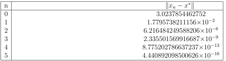
Hence all the conditions of Theorem 4.1 with L = I are satisfied. Therefore, the se-quence {xn} generated by (1.8) is in Br[x0] and it converges to the fixed point x∗ = 3.023785446275295∈Br[x0] of G.
n ∥xn−x∗∥
0 3.0237854462752
1 1.7795738211156×10⁻²
2 6.216484249588206×10⁻⁶
3 2.335501569916687×10⁻⁹
4 8.775202786637237×10⁻¹³
5 4.440892098500626×10⁻¹⁶
Table 1: A priori error bounds
4.2
Fredholm integral equations
fromX into itself. Let S ∈B(X),u∈ X and λ∈F. We investigate a solution x∈X of the nonlinear Fredholm-type operator equation:
x−λSQ(x) = u, (4.2)
where Q : D → X is continuously Fr´echet differentiable on D. The operator equation (4.2) has been discussed in [16], [32] and [35]. Define an operatorF :D→X by
F(x) = x−λSQ(x)−u (4.3) for all x ∈ D. Then solving the operator equation (4.3) is equivalent to solving the operator equation (1.1). From (4.3), we have
Fx′(h) =h−λSQ′x(h) (4.4) for all h∈X. Now, we apply Theorem 3.2 to solve the operator equation (4.2).
Theorem 4.5 LetX be a Banach space and Dan open convex subset ofX. LetQ:D→ X be a continuously Fr´echet differentiable mapping at each point of D. Let L, S ∈B(X)
andu∈X. Assume that, for anyx0 ∈D, z0 =x0−L(x0−λSQ(x0)−u)and(I−λSQ′z0) −1
exist. Assume that the condition (C6) and the following conditions hold:
(C12) (I−L(I−λSQ))(x)−u∈D for all x∈D;
(C13) ∥(I−λSQ′z0)−1∥ ≤β for some β >0;
(C14) ∥(I−λSQ′z0)−1(x0 −λSQ(x0)−u)∥ ≤η for some η >0; (C15) ∥Q′x−Q′y∥ ≤ω0(∥x−y∥) for all x, y ∈D, where ω0 ∈Φ; (C16) ω0(st)≤spω0(t), s∈[0,1] and t ∈[0,∞);
(C17) ∥I−L(I−λSQ′x)∥ ≤k, k≤ 13 for all x∈D. Then we have the following:
(1) The sequence {xn} generated by
zn=xn−L(xn−λSQ(xn)−u),
yn =xn−(I −λSQ′zn)
−1(x
n−λSQ(xn)−u),
xn+1 =yn−(I−λSQ′zn)
−1(y
n−λSQ(yn)−u)
(4.5)
Now, from (C13) and (4.4), we have∥Fz′−01∥ ≤β and so it follows that (C3) holds. From (C14), (4.3) and (4.4), we have ∥F′−1
z0 (F(x0))∥ ≤ η. Hence (C4) is satisfied. For all
x, y ∈D, using (C15), we have
∥Fx′ −Fy′∥ = sup{∥(Fx′ −Fy′)z∥:z ∈X,∥z∥= 1}
≤ |λ|∥S∥sup{∥Q′x−Qy′∥∥z∥:z ∈X,∥z∥= 1}
≤ |λ|∥S∥ω0(∥x−y∥) = ω(∥x−y∥),
whereω(t) = |λ|∥S∥ω0(t). Clearly, ω∈Φ and, from (C16), we have
ω(st)≤spω(t)
for all s ∈ [0,1] and t ∈ (0,∞]. Thus (C1) and (C5) hold. (C2) follows from (C17) for
c=k∈(0,13]. Hence all the conditions of Theorem 3.2 are satisfied. Therefore, Theorem 4.5 follows from Theorem 3.2. This completes the proof.
LetD=X =Y =C[a, b] be the space of all continuous real valued functions defined on [a, b]⊂R with the norm ∥x∥= sup
t∈[a,b]
|x(t)|. Consider, the following nonlinear integral equation:
x(s) =g(s) +λ ∫ b
a
K(s, t)(µx(t)1+p+νx(t)2)dt (4.6) for all s ∈ [a, b] and p ∈ (0,1], where g, x ∈ C[a, b] with g(s) ≥ 0 for all s ∈ [a, b],
K : [a, b]×[a, b] → R is a continuous nonnegative real-valued function and µ, ν, λ ∈ R. Define two mappingsS, Q:D→X by
Sx(s) =
∫ b
a
K(s, t)x(t)dt (4.7)
for all s∈[a, b] and
Qx(s) =µx(s)1+p+νx(s)2 (4.8) for all µ, ν ∈R and s∈[a, b].
One can easily observe thatKis bounded on [a, b]×[a, b], that is, there exists a number
M ≥ 0 such that |K(s, t)| ≤ M for all s, t ∈[a, b]. Clearly, S is bounded linear operator with ∥S∥ ≤M(b−a) and Q is Fr´echet differentiable and its Fr´echet derivative at x∈D
is given by
for all h∈C[a, b]. For all x, y ∈D, we have
∥Q′x−Q′y∥ = sup{∥(Q′x−Q′y)h∥:h∈C[a, b],∥h∥= 1}
≤ sup{∥(µ(1 +p)(xp−yp) + 2ν(x−y))h∥:h∈C[a, b],∥h∥= 1}
≤ sup{(|µ|(1 +p)∥xp−yp∥+ 2|ν|∥x−y∥)∥h∥:h∈C[a, b],∥h∥= 1}
≤ |µ|(1 +p)∥x−y∥p+ 2|ν|∥x−y∥
= ω0(∥x−y∥), (4.10)
whereω0(t) =|µ|(1 +p)tp+ 2|ν|t, t≥0 with
ω0(st)≤spω0(t) (4.11) for all s∈[0,1] andt∈[0,∞). For any x∈D, using (4.7) and (4.9), we have
∥SQ′x∥
= sup{∥SQ′xh∥:h∈X,∥h∥= 1} = sup
{
sup
s∈[a,b]
∫abK(s, t)(µ(1 +p)x(t)p+ 2νx(t))h(t)dt:h∈X,∥h∥= 1
}
≤ sup
{∫ b
a
|K(s, t)|(|µ|(1 +p)|x(t)|p+ 2|ν||x(t)|)|h(t)|dt:h∈X,∥h∥= 1
}
≤ (|µ|(1 +p)∥x∥p + 2|ν|∥x∥)M(b−a)<1. (4.12) We now apply Theorem 4.5 to solve the Fredholm integral equation (4.6).
Theorem 4.6 Let D = X = Y = C[a, b] and µ, ν, λ, M ∈ R. Let S, Q : D → X be operators defined by (4.7) and (4.8), respectively. Let L∈B(X) and x0 ∈D be such that
z0 =x0−L(x0 −λSQ(x0)−g) ∈D. Assume that the condition (C6) and the following
conditions hold:
(C18) 1−|λ|(|µ|(1+p)∥z0∥1p+2|ν|∥z0∥)M(b−a) =β for some β >0;
(C19) ∥x0−g∥+|λ|(|µ|∥x0∥p+1+2|ν|∥x0∥2)M(b−a)
1−|λ|(|µ|(1+p)∥z0∥p+2|ν|∥z0∥)M(b−a) =η for some η >0;
(C20) ∥I−L∥+|λ|∥L∥(|µ|(1 +p)∥x∥p+ 2|ν|∥x∥)M(b−a)≤ 1
3 for all x∈D.
Proof. Note that D=X =Y =C[a, b]. Obviously, (C12) holds. Using (C20), (4.7), (4.9) and (4.12), we have
∥I−(I−λSQ′z0)∥ ≤ |λ|(|µ|(1 +p)∥z0∥p+ 2|ν|∥z0∥)M(b−a)<1. Therefore, by Lemma 2.1, (I−λSQ′z
0)
−1 exists and
∥(I−λSQ′z
0)
−1∥ ≤ 1
1− |λ|(|µ|(1 +p)∥z0∥p + 2|ν|∥z0∥)M(b−a)
. (4.13)
Hence (C18) and (4.13) implies (C13) holds. Using (C19), (4.12) and (4.13), we have
∥(I−λSQ′z0)−1(x0−λSQ(x0)−g)∥
≤ ∥(I−λSQ′z0)−1∥(∥x0−g∥+∥λSQ(x0)∥)
≤ ∥x0−g∥+|λ|(|µ|∥x0∥p+1+ 2|ν|∥x0∥2)M(b−a) 1− |λ|(|µ|(1 +p)∥z0∥p+ 2|ν|∥z0∥)M(b−a)
≤ η.
Thus the condition (C14) is satisfied. The conditions (C15) and (C16) follow from (4.10) and (4.11), respectively. Now, from (C20) and (4.12), we have
∥I−L(I−λSQ′x)∥ ≤ ∥I −L∥+∥L∥∥λSQ′x∥
≤ ∥I −L∥+∥L∥|λ|(|µ|(1 +p)∥x∥p+ 2|ν|∥x∥)M(b−a)
≤ 1
3.
This implies that (C17) holds. Hence all the conditions of Theorem 4.5 are satisfied.
Therefore, Theorem 4.6 follows from Theorem 4.5. This completes the proof. Now, we give one example to illustrate Theorem 4.5.
Example 4.7 Let X =Y =C[0,1] be the space of all continuous real valued functions defined on [0,1]. Let D = {x : x ∈ C[0,1],∥x∥ < 32} ⊂ C[0,1]. Consider the following nonlinear integral equation:
x(s) = sin(πs) + 1 10
∫ 1
0
Define two mappingsS :X →X and Q:D→Y by
S(x)(s) =
∫ 1
0
K(s, t)x(t)dt, Q(x)(s) =x(s)2,
where K(s, t) = cos(πs) sin(πt). For u = sin(πs), the problem (4.14) is equivalent to the problem (4.2). Here, one can easily observe that S is bounded linear operator with
∥S∥ ≤ 1 and Q is Fr´echet differentiable with Q′xh(s) = 2x(s)h(s) for all h ∈ X and
s∈[0,1]. For all x, y ∈D, we have
∥Q′x−Q′y∥ ≤2∥x−y∥=ω0(∥x−y∥),
whereω0(t) = 2t for any t≥0. Clearly, ω0 ∈Φ. Define a mapping F :D→X by
F(x)(s) = x(s)− 1
10SQ(x)(s)−sin(πs).
Clearly, F is Fr´echet differentiable on D. We now show that (C12) holds for L = I ∈ B(X). Note that
∥(I−L(I−λSQ))(x)−u∥= 1
10SQ(x)(s) + sin(πs)
≤ 49
40 < 3 2
for all x∈D. Thus (I−L(I−λSQ))(x)−u∈D for all x∈D. For allx∈D, we have
∥I−Fx′∥ ≤ 1
5∥x∥ ≤ 3 10 =k. Therefore, by Lemma 2.1,Fx′−1 exists and
Fx′−1U(s) = U(s) + cos(πs)
∫1
0 sin(πt)x(t)U(t)dt
5−∫01sin(πt) cos(πt)x(t)dt (4.15)
for all U ∈Y.
Letx0(s) = sin(πs), ω(t) = 101ω0(t) = 5t and p= 1. Then we have the following:
(d) ∥Fz′0−1F(x0)∥ ≤0.050975699850996 =η; (e) b0 =Kβη= 0.012245246321686 and q= 45; (f) θ = (
qb0
2 +k)qb0 2
1−k(1+q)b0 = 5.897481575495280×10
−7 and r = (1+qb0)η
1−θ = 0.091756313844910.
Hence all the conditions of Theorem 4.5 are satisfied. Therefore, the sequence {xn}
generated by (4.5) is well defined, remains in Br[x0] and converges to a solution of the integral equation (4.14).
n xn(s) zn(s) yn(s)
0 sin(πs) sin(πs) + 0.042441318157839 cos(πs) sin(πs)−0.053779425942169 cos(πs) 1 sin(πs)−0.042505426009095 cos(πs) sin(πs)−0.021258998682202 cos(πs) sin(πs)−0.063732700816574 cos(πs) 2 sin(πs) + 0.042457470555443 cos(πs) sin(πs) + 0.021258912220022 cos(πs) sin(πs) + 0.021239768415502 cos(πs) 3 sin(πs) + 0.021230223695582 cos(πs) sin(πs) + 0.021230223705270 cos(πs) sin(πs) + 0.021230223705279 cos(πs) 4 sin(πs) + 0.021230223705279 cos(πs) sin(πs) + 0.021230223705279 cos(πs) sin(πs) + 0.021230223705279 cos(πs)
Table 2: Convergence behavior of Newton-like iteration process (4.5)
Acknowledgements
The second author was supported by Basic Science Research Program through the Na-tional Research Foundation of Korea (NRF) funded by the Ministry of Science, ICT and future Planning (2014R1A2A2A01002100).
References
[1] S. K. Parhi and D. K. Gupta, A third order method for fixed points in Banach spaces, J. Math. Anal. Appl. 359 (2009), 642–652.
[2] S. K Parhi and D. K. Gupta, Convergence of a third order method for fixed points in Banach spaces, Numer. Algorithms 60 (2012), 419–434.
[3] R. P. Agarwal, D. O’Regan and D. R. Sahu, Fixed Point Theory for Lipschitzian-type Mappings with Applications, Series: Topological Fixed Point Theory and its Applications. Springer, New York 6, 2009.