warwick.ac.uk/lib-publications
Manuscript version: Published Version
The version presented in WRAP is the published version (Version of Record).
Persistent WRAP URL:
http://wrap.warwick.ac.uk/128164
How to cite:
The repository item page linked to above, will contain details on accessing citation guidance
from the publisher.
Copyright and reuse:
The Warwick Research Archive Portal (WRAP) makes this work by researchers of the
University of Warwick available open access under the following conditions.
Copyright © and all moral rights to the version of the paper presented here belong to the
individual author(s) and/or other copyright owners. To the extent reasonable and
practicable the material made available in WRAP has been checked for eligibility before
being made available.
Copies of full items can be used for personal research or study, educational, or not-for-profit
purposes without prior permission or charge. Provided that the authors, title and full
bibliographic details are credited, a hyperlink and/or URL is given for the original metadata
page and the content is not changed in any way.
Publisher’s statement:
Please refer to the repository item page, publisher’s statement section, for further
information.
Quantum enhanced estimation of diffusion
Dominic Branford ,1Christos N. Gagatsos,2,1Jai Grover,3Alexander J. Hickey,3and Animesh Datta1
1Department of Physics, University of Warwick, Coventry, CV4 7AL, United Kingdom
2College of Optical Sciences, University of Arizona, 1630 E. University Blvd., Tucson, Arizona 85719, USA
3ESA–Advanced Concepts Team, European Space Research Technology Centre (ESTEC), Keplerlaan 1, Postbus 299,
NL-2200AG Noordwijk, The Netherlands
(Received 14 January 2019; published 30 August 2019)
Momentum diffusion is a possible mechanism for driving macroscopic quantum systems towards classical behavior. Experimental tests of this hypothesis rely on a precise estimation of the strength of this diffusion. We show that quantum-mechanical squeezing offers significant improvements, including when measuring position. For instance, with 10 dB of mechanical squeezing, experiments would require a tenth of proposed free-fall times. Momentum measurement is better by an additional factor of three, while another quadrature is close to optimal. These have particular implications for the space-based MAQRO proposal—where it could rule out the spontaneous collapse theory due to Ghirardi, Rimini, and Weber—as well as terrestrial optomechanical sensing.
DOI:10.1103/PhysRevA.100.022129
I. INTRODUCTION
Finding a unified description of microscopic and macro-scopic systems remains an enduring quest of fundamen-tal physics. One class of proposed solutions are collapse models [1–4] which span continuous spontaneous localiza-tion (CSL) [5–7], Karolyhazy [8], Diósi-Penrose [9–12], and quantum gravity [13], as well as collisional decoherence [14]. In the nonrelativistic regime, they posit spatial decoherence due to diffusion in momentum. The outcome is a description of the evolution in terms of a phase-space density distribution obeying a Fokker-Planck diffusion equation [15]. Experimen-tal advances have now made the testing of this proposition a realistic prospect.
Mechanical systems have been used to bound the strength of such diffusive effects. Examples include gravitational-wave detectors [16], the LISA pathfinder experiment [16–18], ultracold cantilevers [19], and trapped ions [20]. Proposals for future experiments which could probe collapse models and further study macroscopic quantum states include the generation of macroscopic superpositions [21–26] and the space-based MAQRO mission [27,28] which formed a key focus of a recent ESA feasibility study [29].
One simple experiment—which forms a part of the MAQRO mission [27,28]—to test collapse models is to let free particles evolve and measure the expanding width of the wave packet. Once all classical noise sources have been ruled out, any excess wave-packet width must be attributed to momentum diffusion associated with collapse models. MAQRO aims to utilize ultracold nanoparticles and exploit the nanogravity of space to observe free fall over 100 s— enabling more precise sensing of momentum diffusion—as represented in Fig.1.
Quantum techniques such as squeezing allow for more pre-cise estimation [30,31]. Optical squeezing has been identified as valuable to fundamental physics, with squeezing-enhanced interferometry [32] set to enhance laser-interferometric
gravitational-wave detectors [33–35] and 15 dB squeezing of optical vacuum reported [36]. It has also found applica-tion in photonic-force microscopy [37,38], while microwave squeezing is being used in the search for axion dark matter [39]. Quantum squeezing of mechanical degrees of freedom is beginning to be explored in thermal states [40,41].
In this article, we show that quantum squeezing of the me-chanical degree of freedom enables a more precise estimation of the strength of momentum diffusion. This enhancement is attainable with the currently proposed scheme of measuring the position of a particle. We conclude that squeezing can be used to achieve the same precision with reduced free-fall time or center-of-mass cooling. This reduction could be 10-fold for a squeezing of 10 dB. Thus, squeezing can compensate for reduced free-fall times, identified as one of the challenges for MAQRO [27,28] in a recent ESA CDF study [29]. We further show that a momentum measurement is thrice as precise as that of position, while measurement of a more general quadrature is close to optimal. We briefly discuss the potential of the heterodyne and phonon counting measurements.
While our results will be presented in the context of collapse models, observing similar momentum diffusion processes could aid detection of certain dark-matter candi-dates [42–44]. Since excess heating of wave packets is also a consequence of momentum diffusion [20,45,46], our results imply a quantum enhanced estimation of heating. Finally, the ubiquitous phenomena of Brownian motion is also caused by diffusion. Our results can thus be applied in this very general scenario, as well as in particle tracking used to study biological systems [47,48].
(a) (b) (c)
σxx
σxx+τ2σpp
σxx+τ2σpp+τ
3
[image:3.608.51.295.67.156.2]3 λ (d)
FIG. 1. A pictorial representation of the measurement of wave-packet expansion which forms part of the MAQRO propos-als [27,28]. (a) A particle is initially trapped, (b) then released, (c) the free particle wave function expands, more rapidly with a localization term, and (d) the localization rate can be inferred through position measurements. Expansion as depicted in two spatial detections is for illustrative purposes; we analyze only one independent spatial dimension.
quantum-limited estimation of related noise parameters, in-cluding loss [51,52], diffusion in phase shifts [53,54] and displacements [55], and classical stochastic processes [56].
II. BACKGROUND
A particle of mass min a harmonic potential has Hamil-tonian ˆH=Pˆ2/2m+mω2Xˆ2/2.Dimensionless position and momentum operators are ˆx=√mωXˆ/√h¯and ˆp=Pˆ/√hm¯ ω whose commutators are given by the matrixiwhere
= −i
[xˆ,xˆ] [xˆ,pˆ] [pˆ,xˆ] [pˆ,pˆ]
=
0 1
−1 0
. (1)
Quantum states of such a particle have a phase-space representation in terms of the Wigner function of an operator defined as [57, Chap. 1]
Wρ(x,p)= 2
πTr
ρDˆ
x+i p
√
2
ˆ
Dˆ†
x+i p
√
2
, (2)
where ˆD(α)=eαaˆ†−α∗aˆ
and ˆ=eiπaˆ†aˆ
. Gaussian states are those whose Wigner function is Gaussian and so determined by the averages (displacement vectord) and covariances (co-variance matrixσ) of the position and momentum operators. Examples include thermal, coherent, and squeezed states. A thermal state has covariance matrix σ =κth1, with σ =1 corresponding to the ground state.
We focus on the simplest setup to study momentum diffu-sion, that of a free particle as in Fig.1. Initially the particle is trapped in a harmonic potential with frequencyωand cooled. Cooling of nanoparticles has been reported to the order of 100 phonons [58,59] with theory anticipating cooling much closer to the ground state [60,61]. After cooling the trapping poten-tial is turned off. The particle then evolves freely under the Hamiltonian ˆH=Pˆ2/2mwith Lindblad term[Xˆ,[Xˆ, ρ]], whose strength is our parameter of interest. The master equation for momentum diffusion for this system—in terms of the dimensionless position and momentum operators—is
∂ρ ∂τ = −
i 2[pˆ
2, ρ]−1
4λ[xˆ,[ ˆx, ρ]], (3) where τ =ωt andλ=/0 are dimensionless parameters, and 0=mω2/(4 ¯h). Being quadratic the master equation Eq. (3) evolves Gaussian states to Gaussian states [62–64].
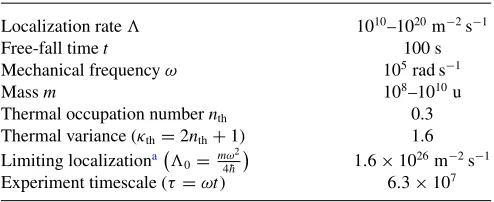
TABLE I. Parameter values based on Kaltenbaek et al. [28], primarily Table 1 therein.
Localization rate 1010–1020m−2s−1
Free-fall timet 100 s
Mechanical frequencyω 105rad s−1
Massm 108–1010u
Thermal occupation numbernth 0.3
Thermal variance (κth=2nth+1) 1.6
Limiting localizationa
0= mω
2
4 ¯h
1.6×1026m−2s−1
Experiment timescale (τ=ωt) 6.3×10⁷
aUsingm=108u.
Equation (3) can then be transformed to a Fokker-Planck equation [63,65], in this case yielding
∂
∂τW(x,p, τ)=
−p∂
∂x+ 1 4λ
∂2 ∂p2
W(x,p, τ), (4)
which for Gaussian W can be mapped to an equation of motion of form [62,64]
∂μ
∂τ =Aμ, ∂σ
∂τ =Aσ +σA T+
D, (5)
where μ andσ are the Gaussian’s moments. For an initial Gaussian state with momentsdandσ the evolved moments under Eq. (4) become
d(τ)=
1 τ 0 1
d, (6)
σ(τ)=
1 τ 0 1 σ 1 0 τ 1 +λ
τ3/3 τ2/2 τ2/2 τ
. (7)
To estimate the strength of the momentum diffusion, we begin with a single-mode Gaussian state. Such a state can be described as a thermal state κth1 with a squeezingr0 of the quadrature ˆxsinφ+pˆcosφ giving an initial covariance matrix
σ =κth
cosh 2r+sinh 2rcos 2φ sinh 2rsin 2φ sinh 2rsin 2φ cosh 2r−sinh 2rcos 2φ
,
(8)
with arbitrary displacements. The displacements do not begin with any parameter dependence and do not gain any through the evolution given by Eq. (6), and so their derivative with respect to the parameter satisfies∂d=0. We will consider tuningφto maximize the precision for given thermal variance and squeezing magnitudes, with φ=0 andφ=π/2 corre-sponding to momentum and position squeezing, respectively.
Our results apply to estimation of diffusion in any scenario governed by Eq. (3) for all values ofλandτ. We will highlight special cases forλ1 andτ 1, which is the regime for MAQRO [27,28] as in TableI, and κth∼1 which is around the MAQRO regime.
[image:3.608.312.559.95.196.2]lower bounds the variance of an unbiased estimator as [66–69]
()2 1
νF() 1
νH(), (9) where ν is the number of repetitions of an experiment, is an estimator of the parameter , and F() and H() are, respectively, the classical Fisher information (CFI) and quantum Fisher information (QFI). The CFI is a function of the probability distribution [66]
F()= dx 1 P(x|ρ)
∂P(x|ρ) ∂
2
, (10)
where the probabilitiesP(x|ρ) are derived from applying
the positive-operator valued measureto the stateρ. The QFI is a function of the state alone [30,31,69]
H()=TrρL2, (11)
where L is the symmetric logarithmic derivative (SLD) defined byLρ+ρL=2∂ρ.
These CFI and QFI provide the CRB and quantum CRB (QCRB), the first and second inequalities of Eq. (9), respec-tively. The equalities in Eq. (9) are obtained by an optimal measurement, where it exists, and an efficient estimator; we identify such a measurement and the maximum likelihood estimator is asymptotically efficient [66].
For a Gaussian state (where ∂d=0) the QFI can be evaluated explicitly as [70,71]
H()= 12(∂σ|(σ⊗σ −⊗)−1|∂σ), (12)
where the inner product is (A|B)=Tr[ATB].
III. RESULTS
Using Eqs. (7) and (8), the QCRB can be calculated through Eq. (12) to be
()2 2 0
κ2
th+τκthλZ+τ 4 12λ2
2
−1
τ4
12
1−κ2
th+τκthλZ+τ 4 12λ2
+τ2
2κ 2 thZ2
, (13)
where Z = (1 + τ2/3) cosh 2r + [(1 − τ2/3) cos 2φ + τsin 2φ] sinh 2r.The bound in Eq. (13) behaves as ()2 2to leading order in.
The QCRB in Eq. (13) is minimized by squeezing or antisqueezing (squeezing the orthogonal quadrature) with squeezing angle (see AppendixA)
φ=arctan
−3+τ2−√9+3τ2+τ4 3τ
, (14)
which tends to 0 for τ 1, corresponding to squeez-ing of position or momentum. When squeezsqueez-ing at this
angle in the regime of τ 1, with κth=1, the QCRB simplifies to
()2208λ
e−2r+τ
4λ
1+τ63e−2rλ+τ4
24λ2
2τ3 3 e−4
r+τ4
3e−2
rλ+τ5
12λ2 ,
with the squeezingrnot necessarily positive as antisqueezing may be preferable (see AppendixA).
Measurement of the particle’s position is a special case of homodyne detection, which involves measuring a linear com-bination of the position and momentum quadratures [64,72]. Heterodyne allows for the simultaneous measurement of posi-tion and momentum, but with added noise [73,74]. The QCRB can be reached through projection onto eigenstates of the SLD [75], which, for a Gaussian system, entails performing some squeezing and displacement followed by measurement of Fock states [51,64,70]. This additional squeezing is a resource applied to the system after the evolution as part of the measurement and does not improve the precision as an initial squeezing can. Further, in a mechanical system this involves measuring the number of phonons, which remains experimen-tally demanding [76,77]. In the following, we calculate the performance of all these measurements for estimating.
Homodyne detection at an angleθmeasures the quadrature ˆ
qθ=xˆcosθ+pˆsinθ. When performed on a Gaussian state the homodyne statistics are Gaussian [72], and the moments are the appropriate marginal of the Wigner function. For a homodyne angleθthe variance of the marginal is
=κth
[(1+τ2) cos2θ+τsin 2θ+sin2θ] cosh 2r
+ {[(1−τ2) cos2θ−τsin 2θ−sin2θ] cos 2φ
+[2τcos2θ+sin 2θ] sin 2φ}sinh 2r
+λ
τ3
3 cos 2θ+τ2
2 sin 2θ+τsin 2θ
, (15)
and as the Wigner function’s mean is parameter-independent, so is the marginal’s. The choices θ=0 andθ=π/2 corre-spond to measurement of position and momentum, respec-tively. We will consider the optimization of θ, which more generally requires measuring a linear combination of the position and momentum operators.
For a Gaussian probability distribution with a parameter-independent mean, the CFI is [66, Chap. 3]
F()= 12Tr−1∂−1∂, (16)
where is the variance of the Gaussian distribution. Using Eqs. (15) and (16), the CRB for homodyne along an angleθ is
()2220
λ+κth
τ2cos2θ+τsin 2θ+1
τ3
3 cos2θ+τ 2
2 sin 2θ+τsin
2θ cosh 2r
−(τ2cos2θ+τsin 2θ−cos 2θ) cos 2φ−
2τcos2θ+sin 2θsin 2φ
τ3
3 cos2θ+τ 2
2 sin 2θ+τsin
2θ sinh 2r
2
To leading order inthis is ()222, which occurs when the first term in the square dominates, whereas when that can be neglected the bound is a-independent constant. The bound on estimating the diffusionfrom position (θ =0) measurement is
()2220
λ+κth
[1+τ2] cosh 2r+ {[1−τ2] cos 2φ+2τsin 2φ}sinh 2r τ3/3
2
, (18)
which behaves as
()2220
λ+κth
cosh 2r−sinh 2rcos 2φ
τ/3
2 , (19)
forτ 1. Instead, for measuring the momentum (θ=π/2) the bound on estimating the diffusionis
()2220
λ+κth
cosh 2r−sinh 2rcos 2φ
τ
2 , (20)
which (neglecting squeezing) matches the large τ limit of position measurements when λκth/τ and is a factor of 9 better whenλκth/τ.
The optimal input squeezing angle φ can in general be found by minimizing the coefficient of sinh 2r in Eq. (17), which gives
φ= −arctan
1
τ+tanθ
. (21)
For momentum measurements (θ=π/2) this squeezing an-gle isφ=0 (squeezing of momentum), whereas for position measurements (θ=0) this isφ= −arctan(1/τ) tending to
φ= −π/2 forτ 1, andφ=0 forτ 1.
In general the squeezing angle in Eq. (21) produces a precision
()2220[λ+κthe−2rχ(τ, θ)]2, (22) from which the unsqueezed case (r=0) can also be extracted, where
χ(τ, θ)= τ
2cos2θ+τsin 2θ+1
τ3
3 cos2θ+τ 2
2 sin 2θ+τsin
2θ. (23)
One effect of squeezing is equivalent to an effective reduction of κth bye−2r. Unlike reducing the center-of-mass motion— which reachesκth=1 at absolute zero—this squeezing allows an unlimited reduction in the second term. Forτ 1 (asχ∼ 1/τ) the same squeezing could instead be considered as an effective increase in τ by a factor ofe2r to obtain the same precision from a much shorter free-fall time.
When the quadrature given by Eq. (21) is squeezed, the homodyne angle which minimizes the bound in Eq. (22) is
θ= −arctan
3+2τ2+√9+3τ2+τ4 3τ
, (24)
which tends to θ ≈ −π/2+1/τ for τ 1. Measuring the quadrature given by Eq. (24) with squeezing as Eq. (21) gives a precision
()2220
λ+κthe−2r
3+τ2−√9+3τ2+τ4 τ3/2
2 .
(25)
Performing homodyne on the quadrature of Eq. (24) does not in general attain the QCRB. Whenλdominates, the QCRB behaves as 2 while any homodyne terms tend to 22. In the τ 1 regime, one could improve on the precision by no more than a factor of 2 using heterodyne detection (see Appendix B). Figure 6 suggests that heterodyne otherwise shows little promise.
Phonon counting—in combination with displacement and squeezing operations—can in principle attain the QCRB for allλandτas the SLD is a quadratic operator in the quadrature operators [64,70] and so has eigenstates which are squeezed-displaced Fock states. The additional squeezing required to attain the QCRB is derived in full generality in AppendixC. For MAQRO, this squeezing seems nugatory, with 79 dB required to attain the QCRB for =1020m−2s−1, which would improve precision only by a factor of√2, to 158 dB for =1010m−2s−1, where the improvement on position measurements would be more pronounced. In other scenarios, however, this could be worthwhile. For τ 1 and λτ21 the squeezing needed is onlye2z≈1+τ ≈1, while forτ
1 andλτ 1 this goes toe2z≈2τ/√3.
IV. DISCUSSION
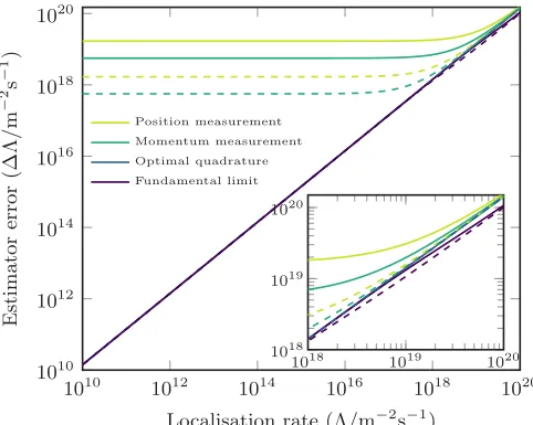
Figure 2 shows the potential improvement in precision for estimating diffusion via momentum or general quadrature measurements, or through squeezing, for MAQRO parameters
1010 1012 1014 1016 1018 1020
1010
1012
1014
1016
1018
1020
Localisation rate (Λ/m−2s−1)
Estimator
error
(ΔΛ
/
m
−
2 s
−
1 )
Position measurement
Momentum measurement
Optimal quadrature
Fundamental limit
1018 1019 1020
1018
1019
[image:5.608.314.555.496.689.2]1020
FIG. 2. Precision of estimating momentum diffusion from wave-packet expansion for MAQRO parameters (TableI). Dashed lines de-note a squeezing of 10 dB. The optimal homodyne and fundamental limit lines overlap until around∼1020m−2s−1. Three years’ data
as given in TableI. For reference, position measurement is the present proposal. We propose squeezing of the momentum quadrature, which offers a substantial improvement across much of the pertinent range for both measurement of position and momentum, with 10 dB enabling an order of magnitude higher resolution of. Measuring the quadrature described by Eq. (24) allows further improvement, keeping within a factor of two of the QCRB across the whole regime.
Our bounds can be mapped to the wealth of diffusive pro-cesses whose parameters enter into the observed diffusion rate
. In the case of (mass-proportional) CSL the two parameters of interest areλCSL andr
C, the time and length scales in the model. The observed diffusion rate for a free sphere of massmand radiusrsis—as a function ofλCSLandrC—given by [28,45]
= λCSL
4r2 C
m m0
2
f
rs
rC
, (26)
where m0 is a reference (nucleon) mass and f(x)= 6
x4[1− 2
x2 +(1+ 2
x2)e− x2
]. From this bounds on λCSL as a function ofrCcan be calculated using
λCSL =4r2 C
m m0
2
f
rs
rC
−1
. (27)
To describe the minimal discernibleλCSLfor measurement of a mechanical quadrature we take the limit of the single-shot CRBλCSL
0 =limλCSL→0λCSL. Allowing forν
indepen-dent repetitions the uncertainty can be reduced toλCSL≈
1 ν
1
ν+1
λCSL
0 atλCSL≈λCSL0 /
√
ν. To ensure any devia-tion can be recognized with statistical significance we take the minimum detectable collapse rateλCSL
min to beλCSLmin ∼√2νλCSL0 . Thus, for a quadrature measurement we take the minimum resolvableλCSLto be given byλCSL
min = 2
√νlimλCSL→0λCSLin
Eq. (17).
For MAQRO such bounds can be seen in Fig. 3 for the position, momentum, and optimal quadratures. For position or momentum measurements with up to 10 dB squeezing the bounds are competitive across 10−8–10−5m; below 10−8m x-ray emission data begin to provide a tighter bound [78], while above 10−5m LISA Pathfinder data are tighter [16,18]. Additional squeezing can of course further reduce the un-certainty, with 20 dB of squeezing sufficient to match the theoretical minimum collapse rate to above 10−7m. This would include testing the original parameters suggested by Ghirardiet al.[15].
The optimal quadrature identified in Eq. (24) meanwhile could yield a conclusive test of the conventional CSL model at a precision of six orders of magnitude more than the theoretical lower bound on CSL [7]. Attaining the QCRB can offer further improvements; however, this would be of little value to MAQRO if the optimal homodyne sensitivity can be reached.
In conclusion, we have shown that squeezing could be used to compensate for reduced free-fall times, an aspect which a recent ESA CDF study [29] has identified as one of the more demanding of the original proposals [27,28]. As, for
10−9 10−7 10−5 10−3 10−1
10−29
10−27
10−25
10−23
10−21
10−19
10−17
10−15
10−13
10−11
Characteristic length (rC/m)
Collapse
rate
(
λ
CSL min
/
s
−
1 )
Position measurement Momentum measurement
Position measurement (10 dB squeezing) Momentum measurement (10 dB squeezing) Optimal quadrature
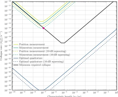
[image:6.608.313.558.67.264.2]Optimal quadrature (10 dB squeezing) Minimum required collapse
FIG. 3. Minimum detectable collapse rate for three years of observation with a 100 nm radius sphere of mass 5.5×10⁹u, with
other parameters as Table I. The minimum required collapse rate given is based on the criteria of Ref. [7] to ensure macroscopic ob-jects rapidly collapse to classical states. The magenta dot represents the values originally proposed by Ghirardiet al.[15].
both Eq. (19) and Eq. (20), the precision is constant fore2rτ
being constant, longer effective free-fall times can be gener-ated through mechanical squeezing. We have also shown the efficacy of momentum and general quadrature measurements over the proposed position measurement.
ACKNOWLEDGMENTS
We thank Rainer Kaltenbaek, Hendrik Ulbricht, Mat-teo Carlesso, and Francesco Albarelli for illuminating dis-cussions. This study has been supported by the European Space Agency’s Ariadna scheme (Study Ref. 17-1201a), the U.K. EPSRC (EP/K04057X/2), and the U.K. Na-tional Quantum Technologies Programme (EP/M01326X/1, EP/M013243/1). D.B. has received support for travel and attendance at workshops from COST Action QTSpace (CA15220).
APPENDIXES
APPENDIX A: OPTIMAL SQUEEZING
1. Fundamental limit
The QCRB is
()2B=20
κ2
th+τκthλZ+τ 4 12λ
22−1
τ4
12
κ2
th+τκthλZ+τ 4 12λ2
+τ4
12
1−2κ2 th
+1
2κth2τ2Z2
, (A1)
where
Z =
1+τ 2
3
cosh 2r+
1−τ 2
3
cos 2φ+τsin 2φ
sinh 2r. (A2)
Minima with respect to the squeezing angle of the bound in Eq. (A1) are either solutions of∂∂BZ =0 or∂∂φZ =0 as
∂B
∂φ = ∂B
∂Z
∂Z
∂φ, (A3)
and the second derivative
∂2B ∂φ2 =
∂2B ∂Z2
∂
Z
∂φ
2
+∂∂B
Z
∂2Z
∂φ2, (A4)
distinguishes minima and maxima. The stationary points ofB(Z) are
Z±=144
1−κ4 th
+24λ2τ41−2κ2 th
+λ4τ8±121−κ2 th
+λ2τ4121+κ2 th
+λ2τ42−48λ2κ2 thτ4 288λκ3
thτ
, (A5)
where the negative root is not possible withr>0 and for the positive root ∂∂2ZB2 <0,and this means that the minimum ofBis
found for ∂∂φZ =0. The stationary points ofZ(φ) are
φ±=arctan
−3+τ2±√9+3τ2+τ4 3τ
, (A6)
where we have
(φ+−φ−) modπ =π
2 (A7)
as tan(φ+) tan(φ−)= −1. Hence we recognize that squeezing the quadrature ˆxφ+is equivalent to antisqueezing of the orthogonal quadrature ˆxφ− =xˆφ++π
2. This follows asr>0 andφ∈[0, π], andr∈Randφ∈[0, π/2] are equivalent parametrizations of
the same squeezings; squeezing a quadrature ˆxφ is equivalent to antisqueezing the quadrature ˆxφ+π/2.
AsB(Z+) is a maximum andZ−<0 is outside the range ofZ(φ) at least one ofφ±is a minimum ofB(φ). We therefore find the global minimum ofB(φ) by finding the smaller ofB(φ+) andB(φ−). ForZ(φ±),
Z(φ±)=
1+τ 2
3
cosh 2r±
√
9+3τ2+τ4 3 sinh 2r
, (A8)
where we note that exchangingφ+ →φ−is equivalent tor→ −r. For these squeezing angles (φ±) the bound [Eq. (A1)] is
()2 20
⎛ ⎝
κ2
th+τκthλ
1+τ 2
3
cosh 2r±
√
9+3τ2+τ4 3 sinh 2r
+τ4
12λ 2 2 −1 ⎞ ⎠ × τ4 12 κ2
th+τκthλ
1+τ 2
3
cosh 2r±
√
9+3τ2+τ4 3 sinh 2r
+τ4
12λ 2
+τ4
12
1−2κth2+τ 2
2 κ 2 th
1+τ 2
3
cosh 2r±
√
9+3τ2+τ4 3 sinh 2r
2⎞
⎠
−1
which can be written as
(a±b)2−1
c±d , (A10)
where
a=κth2 +κthλτ
1+τ 2
3
cosh 2r+τ
4
12λ
2, (A11)
b=κthλτ
√
9+3τ2+τ4
3 sinh 2r, (A12)
c= τ
4
12
1−κth2 +κthλτ
1+τ 2
3
cosh 2r+τ
4
12λ 2
+τ2
2 κ 2 th
1+τ 2
3
2
cosh22r+
1+τ 2
3 +
τ4 9
sinh22r
, (A13)
d =κthλ τ5 12
√
9+3τ2+τ4
3 sinh 2r+κ 2 thτ
2
1+τ 2
3
√
9+3τ2+τ4
3 cosh 2rsinh 2r, (A14) where we havea,b,c, andd all positive as well asa>b+1 andc>d. The squeezing angleφ+ therefore offers a better precision for
c<d
a2+b2−1 2ab
, (A15)
which in this case is
0> λτ
−κ4
th
1+3τ 2
4 +
τ4 9
+τ2
12
1+λ 2τ4
12
2
+κ2 th
τ2 6
1−λ 2τ4
12
+κth
1+τ 2
3
1−κth4 +λ 2τ4
6 (1−2κ 2 th)+
λ2τ4 12
2
cosh 2r−τ
3
6 κ 4
thλcosh 4r. (A16)
2. Homodyne detection
The CRB for homodyne measurement of the quadrature ˆxcosθ+pˆsinθis
()2 220
λ+κth
[1+τ2] cos2θ+τsin 2θ+sin2θ 1
3τ3cos2θ+ 1
2τ2sin 2θ+τsin
2θ cosh 2r
+{[1−τ2] cos2θ−τ1sin 2θ−sin2θ}cos 2φ+ {2τcos2θ+sin 2θ}sin 2φ
3τ3cos2θ+ 1
2τ2sin 2θ+τsin
2θ sinh 2r
2
. (A17)
a. Optimal squeezing
The bound is minimized with respect to the squeezing angleφby minimizing the coefficient of sinh 2r,
[(1−τ2) cos2θ−τsin 2θ−sin2θ] cos 2φ+[2τcos2θ+sin 2θ] sin 2φ, (A18) which has minima
φ= −arctan
1
τ +tanθ
, (A19)
for which squeezing angle the CRB becomes
()2220
λ+e−2rκth
[1+τ2] cos2θ+τsin 2θ+sin2θ 1
3τ3cos2θ+ 1
2τ2sin 2θ+τsin 2θ
2
. (A20)
The optimal homodyne detection can then be recognized as the angleθ
θ= −arctan
3+2τ2+√9+3τ2+τ4 3τ
, (A21)
and when this homodyne angle is used the optimal squeezing angle is
ϕ =arctan
3τ
3−τ2+√9+3τ2+τ4
b. Position and momentum squeezing
Squeezing of position and momentum can be evaluated withφ=0, withr>0 corresponding to squeezing of momentum whiler<0 is a squeezing|r|of position. Forφ=0 the CRB [Eq. (A17)] becomes
()2 220
λ+κth
e2rcos2θ+e−2r(τ2cos2θ+τsin 2θ+sin2θ) 1
3τ3cos2θ+ 1
2τ2sin 2θ+τsin 2θ
2
. (A23)
The optimal homodyne quadrature is then
θ= −arctan
3e4r+2τ2+√9e8r+3e4rτ2+τ4 3τ
, (A24)
which gives a precision
()2 220
λ+κth
2(3e2r+e−2rτ2−√9e4r+3τ2+e−4rτ4) τ3
, (A25)
where squeezing of position (r<0) is beneficial forτ <√3 while squeezing of momentum (antisqueezing of position,r>0) is beneficial forτ >√3.
APPENDIX B: HETERODYNE DETECTION
Heterodyne detection is the projection onto the overcomplete basis of Gaussian states, which amounts to sampling from the Husimi Q function [73,74]. The Q function can be extracted from the Wigner function as [57]
Q(x,p)= 1
π dxd pW(x,p) exp[−(x−x)2−(p−p)2], (B1)
which is a convolution, and so for a Gaussian Wigner function with moments dandσ the Q function will be Gaussian with momentsdandσ+1[64, Chap. 5].
The mean of the distribution again contains no parameter dependence, and so Eq. (16) can also be applied here. The covariances from heterodyne detection are
(τ)=
1+xx+2τx p+τ2pp+13λτ3 x p+τpp+21λτ2 x p+τpp+12λτ2 1+pp+λτ
, (B2)
giving a CRB of
()2 12
2 0|(τ)|2 τ4|(τ)| +6τ21+xx+τx p+τ2
3pp
2
+2τ41+xx−pp−xxpp+2
x p+τ 2
3(1−pp)
, (B3)
where || is the determinant, andxx,x p, andpp are the initial variances and covariance of the position and momentum
operators. Without mechanical squeezing (r=0) this is
()2 6
2 0
(1+κth)2+κthτ2+λ(1+κth)τ
1+τ32+τ124λ22
τ2
3
1+κ2 th
(9+3τ2+τ4)+κ
th(18+6τ2−τ4)
+τ4
2
(1+κth)2+κthτ2+λ(1+κth)τ
1+τ32+τ124λ2. (B4)
APPENDIX C: OPTIMAL MEASUREMENT
For a Gaussian system the SLD is a Hermitian operator, quadratic in the quadrature operators [64,70]. Any such Hermitian operator, quadratic in the quadrature operators, can be transformed through some squeezing and displacement to an operator diagonal in the Fock basis [64,70].
The SLD is primarily defined through identification ofL(2), which is given by [64,70]
which for a state with constant zero displacementsd=0 then gives the SLD [64,70]
Lρ=( ˆx pˆ)L(2)
ˆ x ˆ p
−1
2Tr[L
(2)σ]. (C2)
The covariance matrix which we wish to solve for Eq. (C1) is Eq. (7), which givesL(2)as
L(2)= 1
0(|σ(τ)|2−1)
l(2)
xx lx p(2)
l(2)
x p l(2)pp
, (C3)
where
lxx(2)=τ+τσx p(τ)2−τ2σx p(τ)σpp(τ)+τ3σpp(τ)2, (C4)
lx p(2)= −τσxx(τ)σx p(τ)+ τ2
2 [σxx(τ)σpp(τ)+σx p(τ) 2−
1]−τ 3
3 σx p(τ)σpp(τ), (C5)
lpp(2)=τσxx(τ)2−τ2σxx(τ)σx p(τ)+τ
3
3 [1+σx p(τ)
2]. (C6)
ThenL(2)has eigenvalues
α±
α2−τ2
σxx(τ)−τσx p(τ)+τ
2
3σpp(τ)
2
− τ4
12(|σ(τ)| −1)
2, (C7)
with
α(τ)= τ 2
1+σxx(τ)2−σx p(τ)[σxx(τ)+σpp(τ)]τ + τ2
3[1+σpp(τ) 2]+σ
x p(τ)2
1+τ 2
3
. (C8)
In order for phonon-number-resolving detection to become optimal we then seek the symplectic transformation which gives the Williamson normal form ofL(2). For a single-mode system this can be recognized by first diagonalizingL(2)with a phase shift (−cossinψψ cossinψψ), followed by a squeezing diag(ez,e−z). The phase shift diagonalizesL(2), which has eigenvaluesD
1 and
D2. The symplectic eigenvalue ofL(2) is then
√
D1D2, and so the squeezingz required to bringL(2) into its normal form is
e2z=e12|lnD1−lnD2|.
Thus the required squeezing is
e2z=
1+
1−α12 τ2
σxx(τ)−τσx p(τ)+τ 2 3σpp(τ)
2+τ4
12[|σ(τ)| −1]2
!
1−
1−α12 τ2
σxx(τ)−τσx p(τ)+τ 2 3σpp(τ)
2
+τ4
12[|σ(τ)| −1]2
!. (C9)
10−40 10−20 1 1020 1040
10−40
10−20
1
1020
1040
τ
λ
0
0.2
0.4
0.6
0.8
[image:10.608.43.561.68.352.2]1
FIG. 4. Ratio of quantum Fisher information against classical Fisher information for optimal homodyne quadrature [F(;θopt)/H()], plotted forκth=1 andr=0. The red rectangle
is representative of the MAQRO parameter regime.
10−40 10−20 1 1020 1040
10−40
10−20
1
1020
1040
τ
λ
0
0.2
0.4
0.6
0.8
[image:10.608.220.552.442.665.2]1
FIG. 5. Ratio of quantum Fisher information against classical Fisher information for heterodyne detection [F()/H()], plotted for κth=1 and r=0. The red rectangle is representative of the
APPENDIX D: OPTIMALITY OF DETECTION SCHEMES
Our bounds cover a range of settings with 20 prefac-toring the bounds and their ratios being a function of only
λ, τ, κth, and squeezing reiφ (with parameters such as ho-modyne angle θ representing different measurement choices rather than properties of the system). This allows compar-ison of our bounds in terms of these parameters alone, perhaps the simplest case being where we assume trapping allows us to take κth=1 and that no external squeezing is applied.
1. Homodyne
Forκth=1 and r=0 we can easily compare the QCRB with the optimal homodyne CRB numerically across the λ and τvariables in Fig. 4. The analytic form of the ratio is
10−40 10−20 1 1020 1040
10−40
10−20
1
1020
1040
τ
λ
0 0.5 1
1.5
[image:11.608.316.557.73.239.2]2
FIG. 6. Ratio of classical Fisher information for heterodyne de-tection against classical Fisher information for homodyne dede-tection of the optimal quadrature, plotted forκth=1 andr=0. The red
rectangle is representative of the MAQRO parameter regime.
R= τ
4 λτ1+τ2 3 +τ
3 12λ
+12−1! 721+τ32 +τ63λ−√9+3τ2+τ4
3
2
1+τ32 +τ123λ2−1 2
1+τ321+τ32+τ63λ. (D1)
10−10 10−9 10−8 10−7 10−6 10−5 10−4 10−3 10−2 10−1 100
10−20 10−19 10−18 10−17 10−16 10−15 10−14 10−13 10−12 10−11 10−10 10−9 10−8 10−7 10−6 10−5
Characteristic length (rC/m)
Collapse
rate
(
λ
CSL min
/
s
−
1)
Position measurement Momentum measurement
Position measurement (10 dB squeezing) Momentum measurement (10 dB squeezing) Minimum required collapse
FIG. 7. Bounds plotted for ars=100 nm sphere of mass 5.5×10⁹u with values otherwise as TableI. The minimum required collapse
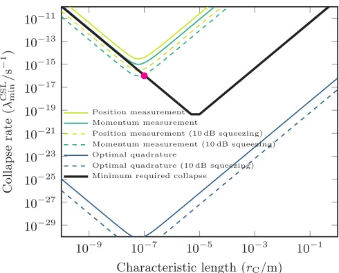
[image:11.608.99.497.354.725.2]10−10 10−9 10−8 10−7 10−6 10−5 10−4 10−3 10−2 10−1 100 10−30
10−29 10−28 10−27 10−26 10−25 10−24 10−23 10−22 10−21 10−20 10−19 10−18 10−17 10−16 10−15 10−14 10−13 10−12 10−11 10−10
Characteristic length (rC/m)
Collapse
rate
(
λ
CSL min
/
s
−
1)
Position measurement Momentum measurement
Position measurement (10 dB squeezing) Momentum measurement (10 dB squeezing) Optimal quadrature
[image:12.608.114.494.71.383.2]Optimal quadrature (10 dB squeezing) Minimum required collapse
FIG. 8. Bounds plotted for ars=100 nm sphere of mass 5.5×10⁹u with values otherwise as TableI. The minimum required collapse
rate given is based on the criteria of Ref. [7]. The magenta dot represents the values originally proposed by Ghirardiet al.[15].
2. Heterodyne
Forκth=1 andr=0 we can easily compare the QCRB with the heterodyne CRB numerically across theλandτ variables in Fig.5. The analytic form of the ratio is
R= λτ
1+τ32 +λτ123+12−1!1+τ32+λτ1232+1+τ622 161+τ2λ21+τ42 +λτ24321+τ32+λτ1232−1
2
1+τ321+τ32 +λτ63. (D2)
3. Homodyne and heterodyne
In the sameκth=1 andr=0 case we can compare the optimal homodyne CRB against the heterodyne CRB numerically across theλandτ variables in Fig.6. This demonstrates no more than a factor of two advantage for heterodyne in theτ 1 andλ1, while in theλ1 regime the homodyne has a near unbounded advantage.
The analytic form of the ratio [which can be seen from Eqs. (D1) and (D2)] is
R= 9
1+τ32 +λτ1232+1+τ6221+τ32+τ63λ− √
9+3τ2+τ4 3
2
2τ41+τ 2λ
2
1+τ42+λτ2432 . (D3)
APPENDIX E: TESTS OF CONTINUOUS SPONTANEOUS LOCALIZATION
For MAQRO the minimum resolvable λCSL for position and momentum can be seen in Fig. 7, plotted for a rs= 100 nm sphere of mass 5.5×10⁹u with values otherwise as TableI, where the black line is based on the minimum required CSL strength proposed in Torošet al.[7]. This plot shows the potential improvements; with MAQRO already competitive
in 10−8–10−5m, squeezing allows a test down to the lower bound for rC<10−7m and significant improvement on re-ported results up torC=10−5m.
limit given by the QCRB will further allow a superior preci-sion through a saturating measurement. Such improvements,
however, offer little significance, as the QCRB will give a lower bound no less than that of the optimal quadrature.
[1] A. Bassi and G. Ghirardi, Dynamical reduction models,Phys. Rep.379,257(2003).
[2] A. Bassi, K. Lochan, S. Satin, T. P. Singh, and H. Ulbricht, Models of wave-function collapse, underlying theories, and experimental tests,Rev. Mod. Phys.85,471(2013).
[3] A. Bassi, D. Dürr, and G. Hinrichs, Uniqueness of the Equa-tion for Quantum State Vector Collapse,Phys. Rev. Lett.111,
210401(2013).
[4] A. Bassi, A. Großardt, and H. Ulbricht, Gravitational decoher-ence,Classical Quant. Grav.34,193002(2017).
[5] P. Pearle, Combining stochastic dynamical state-vector reduc-tion with spontaneous localizareduc-tion, Phys. Rev. A 39, 2277
(1989).
[6] G. C. Ghirardi, P. Pearle, and A. Rimini, Markov processes in Hilbert space and continuous spontaneous localization of systems of identical particles,Phys. Rev. A42,78(1990). [7] M. Toroš, G. Gasbarri, and A. Bassi, Colored and dissipative
continuous spontaneous localization model and bounds from matter-wave interferometry,Phys. Lett. A381,3921(2017). [8] F. Karolyhazy, Gravitation and quantum mechanics of
macro-scopic objects,Nuovo Cimento A (1965–1970)42,390(1966). [9] L. Diósi, A universal master equation for the gravitational violation of quantum mechanics,Phys. Lett. A120,377(1987). [10] L. Diósi, Models for universal reduction of macroscopic
quan-tum fluctuations,Phys. Rev. A40,1165(1989).
[11] R. Penrose, On gravity’s role in quantum state reduction,Gen. Relativ. Grav.28,581(1996).
[12] M. Bahrami, A. Smirne, and A. Bassi, Role of gravity in the collapse of a wave function: A probe into the Diósi-Penrose model,Phys. Rev. A90,062105(2014).
[13] J. Ellis, S. Mohanty, and D. V. Nanopoulos, Quantum gravity and the collapse of the wavefunction,Phys. Lett. B221,113
(1989).
[14] M. R. Gallis and G. N. Fleming, Environmental and sponta-neous localization,Phys. Rev. A42,38(1990).
[15] G. C. Ghirardi, A. Rimini, and T. Weber, Unified dynamics for microscopic and macroscopic systems, Phys. Rev. D34, 470
(1986).
[16] M. Carlesso, A. Bassi, P. Falferi, and A. Vinante, Experimental bounds on collapse models from gravitational wave detectors,
Phys. Rev. D94,124036(2016).
[17] B. Helou, B. J. J. Slagmolen, D. E. McClelland, and Y. Chen, LISA pathfinder appreciably constrains collapse models,Phys. Rev. D95,084054(2017).
[18] M. Carlesso, M. Paternostro, H. Ulbricht, A. Vinante, and A. Bassi, Non-interferometric test of the continuous spontaneous localization model based on rotational optomechanics,New J. Phys.20,083022(2018).
[19] A. Vinante, R. Mezzena, P. Falferi, M. Carlesso, and A. Bassi, Improved Noninterferometric Test of Collapse Models Using Ultracold Cantilevers,Phys. Rev. Lett.119,110401(2017). [20] Y. Li, A. M. Steane, D. Bedingham, and G. A. D. Briggs,
Detecting continuous spontaneous localization with charged bodies in a Paul trap,Phys. Rev. A95,032112(2017).
[21] O. Romero-Isart, A. C. Pflanzer, F. Blaser, R. Kaltenbaek, N. Kiesel, M. Aspelmeyer, and J. I. Cirac, Large Quantum Superpositions and Interference of Massive Nanometer-Sized Objects,Phys. Rev. Lett.107,020405(2011).
[22] O. Romero-Isart, Quantum superposition of massive ob-jects and collapse models, Phys. Rev. A 84, 052121
(2011).
[23] M. Scala, M. S. Kim, G. W. Morley, P. F. Barker, and S. Bose, Matter-Wave Interferometry of a Levitated Thermal Nano-Oscillator Induced and Probed by a Spin,Phys. Rev. Lett.111,
180403(2013).
[24] C. Wan, M. Scala, G. W. Morley, ATM. A. Rahman, H. Ulbricht, J. Bateman, P. F. Barker, S. Bose, and M. S. Kim, Free Nano-Object Ramsey Interferometry for Large Quantum Superpositions,Phys. Rev. Lett.117,143003(2016).
[25] S. Bose, A. Mazumdar, G. W. Morley, H. Ulbricht, M. Toroš, M. Paternostro, A. A. Geraci, P. F. Barker, M. S. Kim, and G. Milburn, Spin Entanglement Witness for Quantum Gravity,
Phys. Rev. Lett.119,240401(2017).
[26] M. J. Weaver, D. Newsom, F. Luna, W. Löffler, and D. Bouwmeester, Phonon interferometry for measuring quantum decoherence,Phys. Rev. A97,063832(2018).
[27] R. Kaltenbaek, G. Hechenblaikner, N. Kiesel, O. Romero-Isart, K. C. Schwab, U. Johann, and M. Aspelmeyer, Macroscopic quantum resonators (MAQRO),Exp. Astron.34,123(2012). [28] R. Kaltenbaek, M. Aspelmeyer, P. F. Barker, A. Bassi, J.
Bateman, K. Bongs, S. Bose, C. Braxmaier, ˇC. Brukner, B. Christophe, M. Chwalla, P.-F. Cohadon, A. M. Cruise, C. Curceanu, K. Dholakia, L. Diósi, K. Döringshoff, W. Ertmer, J. Gieseler, N. Gürlebeck, G. Hechenblaikner, A. Heidmann, S. Herrmann, S. Hossenfelder, U. Johann, N. Kiesel, M. Kim, C. Lämmerzahl, A. Lambrecht, M. Mazilu, G. J. Milburn, H. Müller, L. Novotny, M. Paternostro, A. Peters, I. Pikovski, A. Pilan-Zanoni, E. M. Rasel, S. Reynaud, C. J. Riedel, M. Rodrigues, L. Rondin, A. Roura, W. P. Schleich, J. Schmiedmayer, T. Schuldt, K. C. Schwab, M. Tajmar, G. M. Tino, H. Ulbricht, R. Ursin, and V. Vedral, Macroscopic quan-tum resonators (MAQRO): 2015 update,EPJ Quant. Tech.3,5
(2016).
[29] European Space Agency, CDF study report: QPPF— Assessment of a quantum physics payload platform, Tech. Rep. CDF-183(C), European Space Agency (2018).
[30] G. Tóth and I. Apellaniz, Quantum metrology from a quan-tum information science perspective,J. Phys. A 47, 424006
(2014).
[31] R. Demkowicz-Dobrza´nski, M. Jarzyna, and J. Kołody´nski, Quantum limits in optical interferometry, inProgress in Op-tics, Vol. 60, edited by E. Wolf (Elsevier, Amsterdam, 2015), pp. 345–435.
[32] C. M. Caves, Quantum-mechanical noise in an interferometer,
Phys. Rev. D23,1693(1981).
[34] H. Grote, K. Danzmann, K. L. Dooley, R. Schnabel, J. Slutsky, and H. Vahlbruch, First Long-Term Application of Squeezed States of Light in a Gravitational-Wave Observatory,Phys. Rev. Lett.110,181101(2013).
[35] The LIGO Scientific Collaboration, Enhanced sensitivity of the LIGO gravitational wave detector by using squeezed states of light,Nat. Photonics7,613(2013).
[36] H. Vahlbruch, M. Mehmet, K. Danzmann, and R. Schnabel, Detection of 15 dB Squeezed States of Light and Their Appli-cation for the Absolute Calibration of Photoelectric Quantum Efficiency,Phys. Rev. Lett.117,110801(2016).
[37] M. A. Taylor, J. Knittel, and W. P. Bowen, Fundamental con-straints on particle tracking with optical tweezers,New J. Phys. 15,023018(2013).
[38] M. A. Taylor, J. Janousek, V. Daria, J. Knittel, B. Hage, H.-A. Bachor, and W. P. Bowen, Subdiffraction-Limited Quantum Imaging within a Living Cell,Phys. Rev. X4,011017(2014). [39] M. Malnou, D. A. Palken, B. M. Brubaker, L. R. Vale, G. C.
Hilton, and K. W. Lehnert, Squeezed Vacuum Used to Accel-erate the Search for a Weak Classical Signal,Phys. Rev. X9,
021023(2019).
[40] A. Pontin, M. Bonaldi, A. Borrielli, F. S. Cataliotti, F. Marino, G. A. Prodi, E. Serra, and F. Marin, Squeezing a Thermal Mechanical Oscillator by Stabilized Parametric Effect on the Optical Spring,Phys. Rev. Lett.112,023601(2014).
[41] M. Rashid, T. Tufarelli, J. Bateman, J. Vovrosh, D. Hempston, M. S. Kim, and H. Ulbricht, Experimental Realization of a Thermal Squeezed State of Levitated Optomechanics, Phys. Rev. Lett.117,273601(2016).
[42] C. J. Riedel, Direct detection of classically undetectable dark matter through quantum decoherence,Phys. Rev. D88,116005
(2013).
[43] C. J. Riedel, Decoherence from classically undetectable sources: Standard quantum limit for diffusion,Phys. Rev. A92,
010101(R)(2015).
[44] C. J. Riedel and I. Yavin, Decoherence as a way to measure extremely soft collisions with dark matter, Phys. Rev. D 96,
023007(2017).
[45] B. Collett and P. Pearle, Wavefunction collapse and random walk,Found. Phys.33,1495(2003).
[46] L. Diósi, Testing Spontaneous Wave-Function Collapse Mod-els on Classical Mechanical Oscillators,Phys. Rev. Lett.114,
050403(2015).
[47] L. P. Ghislain and W. W. Webb, Scanning-force microscope based on an optical trap,Opt. Lett.18,1678(1993).
[48] A. Pralle, E.-L. Florin, E. Stelzer, and J. Hörber, Local viscosity probed by photonic force microscopy,Appl. Phys. A66,S71
(1998).
[49] M. G. Genoni, O. S. Duarte, and A. Serafini, Unravelling the noise: The discrimination of wave function collapse models under time-continuous measurements,New J. Phys.18,103040
(2016).
[50] S. McMillen, M. Brunelli, M. Carlesso, A. Bassi, H. Ulbricht, M. G. A. Paris, and M. Paternostro, Quantum-limited estima-tion of continuous spontaneous localizaestima-tion,Phys. Rev. A95,
012132(2017).
[51] A. Monras and M. G. A. Paris, Optimal Quantum Estimation of Loss in Bosonic Channels,Phys. Rev. Lett.98,160401(2007). [52] G. Adesso, F. Dell’Anno, S. De Siena, F. Illuminati, and L. A. M. Souza, Optimal estimation of losses at the ultimate
quantum limit with non-Gaussian states, Phys. Rev. A 79,
040305(R)(2009).
[53] S. I. Knysh and G. A. Durkin, Estimation of phase and diffusion: Combining quantum statistics and classical noise,
arXiv:1307.0470.
[54] M. D. Vidrighin, G. Donati, M. G. Genoni, X.-M. Jin, W. S. Kolthammer, M. S. Kim, A. Datta, M. Barbieri, and I. A. Walmsley, Joint estimation of phase and phase diffusion for quantum metrology,Nat. Commun.5,3532(2014).
[55] M. Tsang, Quantum limit to subdiffraction incoherent optical imaging,Phys. Rev. A99,012305(2019).
[56] S. Ng, S. Z. Ang, T. A. Wheatley, H. Yonezawa, A. Furusawa, E. H. Huntington, and M. Tsang, Spectrum analysis with quan-tum dynamical systems,Phys. Rev. A93,042121(2016). [57] A. Ferraro, S. Olivares, and M. G. A. Paris, Gaussian states in
continuous variable quantum information (Bibliopolis, Napoli, 2005),arXiv:quant-ph/0503237.
[58] D. Windey, C. Gonzalez-Ballestero, P. Maurer, L. Novotny, O. Romero-Isart, and R. Reimann, Cavity-Based 3D Cooling of a Levitated Nanoparticle Via Coherent Scattering,Phys. Rev. Lett.122,123601(2019).
[59] U. Deli´c, M. Reisenbauer, D. Grass, N. Kiesel, V. Vuleti´c, and M. Aspelmeyer, Cavity Cooling of a Levitated Nanosphere by Coherent Scattering,Phys. Rev. Lett.122,123602(2019). [60] O. Romero-Isart, L. Clemente, C. Navau, A. Sanchez, and J. I.
Cirac, Quantum Magnetomechanics with Levitating Supercon-ducting Microspheres,Phys. Rev. Lett.109,147205(2012). [61] C. Gonzalez-Ballestero, P. Maurer, D. Windey, L. Novotny, R.
Reimann, and O. Romero-Isart, Theory for cavity cooling of levitated nanoparticles via coherent scattering: Master equation approach,Phys. Rev. A100,013805(2019).
[62] H. J. Carmichael, Statistical Methods in Quantum Optics 1: Master Equations and Fokker-Planck Equations, Theoretical and Mathematical Physics (Springer-Verlag, Berlin, 1999). [63] F. Nicacio, R. N. P. Maia, F. Toscano, and R. O. Vallejos, Phase
space structure of generalized Gaussian cat states,Phys. Lett. A 374,4385(2010).
[64] A. Serafini,Quantum Continuous Variables: A Primer of Theo-retical Methods(CRC Press, Boca Raton, 2017).
[65] S. M. Barnett and P. M. Radmore, Methods in Theoretical Quantum Optics(Oxford University Press, Oxford, 2002). [66] S. M. Kay, Fundamentals of Statistical Signal Processing:
Estimation Theory(Prentice-Hall PTR, New York, 1998). [67] C. W. Helstrom, Quantum Detection and Estimation Theory
(Academic Press, New York, 1976).
[68] A. Holevo,Probabilistic and Statistical Aspects of Quantum Theory(Edizioni della Normale, Pisa, 2011).
[69] M. G. A. Paris, Quantum estimation for quantum technology,
Int. J. Quant. Inform.7,125(2009).
[70] A. Monras, Phase space formalism for quantum estimation of Gaussian states,arXiv:1303.3682.
[71] D. Šafránek, A. R. Lee, and I. Fuentes, Quantum parameter estimation using multi-mode Gaussian states,New J. Phys.17,
073016(2015).
[72] G. Adesso, S. Ragy, and A. R. Lee, Continuous variable quan-tum information: Gaussian states and beyond,Open Syst. Inf. Dyn.21,1440001(2014).
[73] J. Shapiro and S. Wagner, Phase and amplitude uncertainties in heterodyne detection,IEEE J. Quantum Electron. 20, 803
[74] U. Leonhardt and H. Paul, Measuring the quantum state of light,
Prog. Quantum Electron.19,89(1995).
[75] S. L. Braunstein and C. M. Caves, Statistical Distance and the Geometry of Quantum States,Phys. Rev. Lett.72,3439(1994). [76] J. D. Cohen, S. M. Meenehan, G. S. MacCabe, S. Gröblacher, A. H. Safavi-Naeini, F. Marsili, M. D. Shaw, and O. Painter, Phonon counting and intensity interferometry of a nanomechan-ical resonator,Nature (London)520,522(2015).
[77] S. Hong, R. Riedinger, I. Marinkovi´c, A. Wallucks, S. G. Hofer, R. A. Norte, M. Aspelmeyer, and S. Gröblacher, Hanbury Brown and Twiss interferometry of single phonons from an optomechanical resonator,Science358,203(2017).
[78] K. Piscicchia, A. Bassi, C. Curceanu, R. D. Grande, S. Donadi, B. C. Hiesmayr, and A. Pichler, CSL collapse model mapped with the spontaneous radiation, Entropy 19, 319
![FIG. 4. Ratioofclassical Fisher information for optimal homodyne quadrature[F(quantumFisherinformationagainst�; θopt)/H(�)], plotted for κth = 1 and r = 0](https://thumb-us.123doks.com/thumbv2/123dok_us/9421640.445234/10.608.43.561.68.352/ratioofclassical-fisher-information-optimal-homodyne-quadrature-quantumfisherinformationagainst-plotted.webp)