Pre Decision Side Bet Sequences

Economics Working Paper Series

2017/010

Pre-Decision Side-Bet Sequences

Kim Kaivanto and David Peel

The Department of Economics

Lancaster University Management School

Lancaster LA1 4YX

UK

© Authors

All rights reserved. Short sections of text, not to exceed two paragraphs, may be quoted without explicit permission,

provided that full acknowledgement is given.

Pre-Decision Side-Bet Sequences

Kim Kaivanto∗and David Peel

Department of Economics, Lancaster University, Lancaster LA1 4YX, UK

this version: April 6, 2017

Abstract

Risk-averse Expected Utility (EU) decision makers with wealth-dependent utility functions may

find themselves indifferent between accepting and rejecting an indivisible risky prospect. Bell

(1988) showed that under these circumstances it is EU-enhancing for the decision maker to

engage in a pre-decision side bet, accepting the indivisible risky prospect conditional upon

winning the side bet. The side bet places the decision maker on the convex hull between the

initial-wealth utility function and the utility function with risky-prospect-augmented wealth.

We show that decision makers restricted to actuarially unfair side bets engage in a sequence

of individually EU-enhancing side bets. This occurs because optimal stake size is modest for

actuarially unfair side bets, whereby wealth remains within the interval of interim convexity

upon losing the side bet. As optimal stake size falls strongly with each successive side-bet

round, wealth remains within the interval of interim convexity. The EU enhancement conferred

by each successive round is also strongly diminishing. Hence the side-bet sequence is eventually

truncated when no further EU enhancement is available.

Keywords: Expected Utility, risk aversion, side bets, rationality, indivisibility, discreteness,

actuarial fairness

JEL classification: D81

1 Introduction

Early in the development of modern Expected Utility (EU) theory, the descriptive value and

behavioral implications of utility-function convexity was acutely appreciated (Friedman and

Savage, 1948; Markowitz, 1952). However once the normative approach took hold in modern

EU theory, globally concave utility functions became the primary focus of investigation. It took

a further forty years before Bell (1988) showed that local convexity can emerge on an interim

basis for globally risk-averse decision makers who are in possession of a standing offer to acquire

a discrete, indivisible risky prospect. Global risk aversion notwithstanding, then, a normatively

rational EU decision maker can benefit by increasing her risk exposure through a pre-decision

side bet when within such a region of interim local convexity (Bell, 1988).1 _{This seemingly}

counterintuitive result applies in the neighborhood of any wealth level at which a risky prospect

switches from being EU-diminishing to being EU-augmenting. Thus it holds for all EU decision

makers possessing such switch points – i.e. all but those with linear or exponential utility

functions.

We show that when a decision maker has access to actuarially unfair side bets, the optimal

side bet’s stake is smaller than in the actuarially fair case. When the decision maker loses an

optimal actuarially fair side bet, she is ejected to the lower bound of the interval of interim

convexity. However in the event of losing an actuarially unfair side bet, the decision-maker’s

wealth is diminished, but not by enough to fall out of the interval of interim convexity. Hence, a

second optimally EU-enhancing side bet may be constructed, the stake of which is smaller than

that of the first side bet, keeping the decision maker within the interval of interim convexity.

When the decision maker is indifferent between her initial certain wealth and acquiring the

indivisible risky prospect, not only will it be possible to construct a single actuarially unfair

optimal side bet, but in general a sequence of individually optimal actuarially unfair side bets

may be constructed, given continual availability of the side bets at ever-longer odds.

1

2 Single side bet

We follow Bell (1988) in illustrating the singe-side-bet case with a logarithmic-utility example in

which the decision maker’s initial wealth is w0 = $10,000. The decision maker is in possession

of a standing offer to acquire the risky prospect g0 = ($15,000,1₂; $0,1₂) for the stub price of

$5,000. We write the prospect in net-final-wealth terms as g(g0, w0) = ($20,000,1₂; $5,000,1₂).

Define this to be the round-zero lottery L0 =g(g0, w0). Since

E[u(L0)] = 1₂ln($20,000) +1₂ln($5,000) = ln($10,000) =u(w0) (1)

the decision maker is indifferent between acquiring the risky prospect and sticking with her

initial (certain) wealth.

Now let the decision maker consider a pre-decision side bet g1 = ($1,000,1₂;−$1,000,1₂).

Although g1 and g0 are stochastically independent, the decision maker considers a compound,

conditional policy of only acquiring the round-zero lottery L0 if the side bet proves successful.

This compound lottery, which presumes the Reduction of Compound Lotteries (ROCL) axiom,

may be written as follows.

L1(g(g0, w0), g1) = $21,000,1₄; $6,000,1₄; $9,000,1₂

(2)

Although the side bet g1 is EU-diminishing in isolation due to risk aversion, when g0 is

im-plemented conditional upon successful resolution of g1, the resulting compound lottery is

EU-augmenting.

E[u(L1)] = 1₄ln($21,000) +1₄ln($6,000) +1₂ln($9,000) > ln($10,000) =u(w0) (3)

The Certainty Equivalent (CE) of this compound lottery is $10,002.2 _{This is a marginal ($2)}

improvement, reflecting the arbitrary nature of the side bet g1. By appropriate choice of the

side bet, it will in principle be possible to improve upon this CE. Two classes of solutions are

of interest: unconstrained optimal side bets g∗

1, and counterparty-constrained optimal side bets

g∗1|s,µ. In the former, the side-bet counterparty limits neither the maximum stake s nor the

2

expected return on a unit stake, i.e. the maximum mean return µ. In the latter, the side-bet

counterparty may impose a ceiling on the maximum permissible stake, and/or on the maximum

mean returnµ < 0, which captures the actuarially unfair odds associated with ‘house edge’. If

the counterparty is a casino, table limits impose a ceiling on the maximum stake, and the mean

return is limited toµ=−₃₇1 (European roulette) orµ=−₁₉1 (American roulette).

An EU-augmenting side bet can be constructed only if the decision maker’s wealth falls

within the interval of interim convexity. The bounds of this interval also determine the payoffs

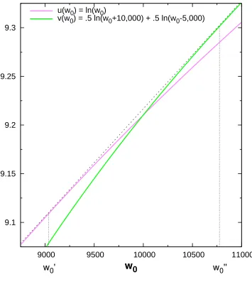
and probabilities of the optimal side bet. Figure 1 illustrates the decision-maker’s utility function

u(·) without the risky prospect and v(·) with the risky prospect. The common tangent to u(·)

and v(·) identifies the lower and upper bounds of the interval of interim convexity (w₀′, w₀′′). The solution method for identifying these bounds analytically is presented in Appendix A. This

yields the numerical values (w0′, w′′0) = (9037.16,10774.6). Given the decision-maker’s assumed

wealth in this example, an EU-augmenting side bet is possible since 10,000∈(9037.16,10774.6),

and the unconstrained optimal side bet is given by g∗1 = (w0′′−w0, w0−w′0

w′′

0−w′0; w

′

0−w0, w′′

0−w0

w′′

0−w′0) =

($774.6,0.554; −$962.84,0.446). With this optimal pre-decision side bet g∗

1, the compound

lottery becomes

L1(g(g0, w0), g1∗) = ($20774.6,0.277; $5774.6,0.277; $9037.16,0.446) (4)

and the decision maker increases her utility

E[u(L1(g(g0, w0), g∗1))] > E[u(L1(g(g0, w0), g1))] > u(w0) (5)

to the CE wealth level of $10,052.8, which is clearly greater than the $10,002 of the arbitrary

side betg0.

We may also develop a counterparty-constrained optimal-side-bet example which recognizes

that large-scale providers of side-bet services – gaming industry firms – typically do so on an

actuarially unfair basis, or with limits (e.g. table limits) that protect consumers from themselves

and the house against doubling strategies. Here we focus on the restriction to actuarially unfair

side bets, specifically in the form of theµ=−₃₇1 unit-bet expected return in European roulette.3

3

Figure 1: Common tangent to u(·) and v(·) which determines the bounds of the interval of interim convexity (w′

0, w′′0) for the round-one side bet.

9.1 9.15 9.2 9.25 9.3

9000 9500 10000 10500 11000

w

w

'

w

''

u(w₀) = ln(w₀)

v(w₀) = .5 ln(w₀+10,000) + .5 ln(w₀-5,000)

Denote the (actuarially unfair) house payout odds by a. For a single-number bet in European

roulette, the payout odds are 35:1, that is a= 35

1. The associated win probability is p= 1+µ 1+a,

which for the single-number bet isp= (1 +−1 37)/(1 +

35 1) =

1

37. Meanwhile, the interim-convexity

bounds remain as above.4 _{To determine the optimal round-one counterparty-constrained optimal}

side bet, we maximize

p

1

2ln(w0+ 10,000 +sa) + 1

2ln(w0−5,000 +sa)

+ (1−p) ln(w0−s) (6)

by appropriate choice of stake s and payout odds a. As the win probability p is a function

against the number turning up are 36:1⇔p= 1 37. 4

of a and the fixed parameter µ, there are no other undetermined parameters. This is solved

by setting s = 573.33 and sa = 732.77 – i.e. smaller than in the unconstrained, actuarially

fair problem – from which follows that a = 732.77/573.33 = 1.27809 and consequently p =

(1−(1/37))/(1 + 1.27809) = 0.42710. Due to the house advantageµ= −₃₇1, the expected value of this side bet is|µ|s= $15.50 less than in the unconstrained problem, i.e. E[w0+psa−(1−p)s] =

$10,000−$15.50 = $9,984.50.

L1(g(g0, w0), g∗1|µ) = ($20732.77,0.21355; $5732.77,0.21355; $9,426.67,0.5729) (7)

With the optimal counterparty-constrained pre-decision side betg∗₁|µ, the CE of this compound

lottery (7) becomes $10,030.69, in which the $30.69 increase over the pre-side-bet CE is 58% of

the $52.80 increase achieved with the actuarially fair side bet g∗1. Still, with the

counterparty-constrained optimal side bet g1∗|µ the compound lottery L1(g(g0, w0), g1∗|µ) nevertheless proves

to be EU-augmenting.

E[u(L1(g(g0, w0), g1∗))] > E[u(L1(g(g0, w0), g1∗|µ))] > E[u(L1(g(g0, w0), g1))] > u(w0)

(8)

3 Sequences of individually optimal side bets

3.1 Counterparty-unconstrained, actuarially fair case

After losing the side betg1∗ in the round-one compound lottery L1(g(g0, w0), g1∗) and therefore

the $962.84 stake, the decision-maker’s wealth is reduced to w1 = w′0 = 9037.16. Although it

is possible to solve for the optimal round-two counterparty-unconstrained side bet,5 _{this side}

bet is EU diminishing. Hence for the counterparty-unconstrained case, the side-bet sequence is

degenerate, being truncated atg∗

1 as in Bell (1988). This degeneracy does not carry over to the

counterparty-constrained case, however.

5

g∗

2= ($1,733.17,7.3765×10− 4

3.2 Actuarially unfair case

When side bets are constrained to be actuarially unfair, the round-one side-bet stake is smaller

than the difference between initial wealthw0and the lower bound of the interval of convexityw′0.

Hence, after losing the side betg∗

1|µ in the round-one compound lottery L1(g(g0, w0), g∗1|µ) and

therefore the associated stake s∗

1µ = $573.33, the decision-maker’s wealth is reduced to w1 =

$9,426.67 ∈(w′₀, w₀′′), which is within the interval of convexity. Consequently the decision-maker can benefit from a further side-bet round. In turn the stake of the optimal round-two side bet

s∗_2µ= $135.25 is also smaller thanw1−w′0. Upon losing the side bet of the round-two compound

lotteryL2(g(g0, w1), g2∗|µ), the decision-maker’s wealth is reduced tow2 = $9,291.43 ∈(w0′, w0′′),

which is within the interval of convexity. Again the decision maker can benefit from a further

side-bet round. Table 1a presents this sequence of individually EU-augmenting optimal side

bets against a European-roulette counterparty. These side bets have been computed under the

assumption that the minimum stake-size increment is 0.01 (one penny). The round-four side

bet’s CE∗

4µ is larger than w3 in the fourth decimal digit. Similarly CE ∗

5µ > w4 in the sixth

decimal digit, and CE∗_6µ > w5 in the eighth decimal digit. Notice that availability of

ever-longer-odds side bets is necessary for extending the sequence, which nevertheless is truncated

to six rounds due to the discrete, one-penny stake-size increment.

Table 1a also presents the operator’s sum of expected payoffs |µ|s∗_iµQi−1

j=0qj, where qi =

(1−pi) = 1−((1 +µ)/(1 +a∗_iµ)) is the probability that the decision maker loses her ith side

bet to the operator.6 _q

i−1 is the probability that the decision maker loses heri−1 side bet, and

consequently finds herself undertaking the EU-enhancing side bet in roundi. The column total

$17.89 in Table 1a is the gaming operator’s expected gross revenue from the decision maker’s

sequence of individually rational side bets.

Table 1b presents the sequence of individually EU-augmenting optimal side bets against an

American-roulette counterparty. Due to the more disadvantagous mean return (µ = −₁₉1), the round-one stake is considerably smaller than when the counterparty operates a European roulette

wheel ($358.83 rather than $573.33). After this initial stake is lost, wealth remains closer to the

original point of indifference (i.e. w0 = $10,000). Hence, subsequent-round stakes are larger

than in theµ= −1

37 case. However,µ=

−1

19 supports fewer individually utility-enhancing rounds

6

Table 1: Parameters of optimal EU-augmenting round-iside bets.

(a) European roulette (µ=−1 37).

i wi−1 s∗_iµ a∗_iµ |µ|s∗_iµ CE∗_iµ |µ|s∗_iµ

Qi−1 j=0qj

1 10,000.00 573.33 1.28 15.49 10,030.69 15.49

2 9,426.67 135.25 9.85 3.66 9,428.03 2.10

3 9,291.42 19.41 75.58 0.52 9,291.45 0.27

4 9,272.01 1.80 827.27 0.05 >9,272.01 0.03 5 9,270.21 0.23 6482.14 0.01 >9,270.21 0.00

6 9,269.98 0.03 49702.21 0.00 >9,269.98 0.00

P

730.05 19.73 17.89

(b) American roulette (µ=−1 19).

i wi−1 s∗_iµ a∗_iµ |µ|s∗_iµ CE∗_iµ |µ|s∗_iµ Qi₋1

j=0qj

1 10,000.00 358.83 1.82 18.86 10,017.53 18.86

2 9,641.17 131.89 8.10 6.94 9,642.96 4.61

3 9,509.28 30.43 39.16 1.60 9,509.39 0.95

4 9,478.85 9.76 127.33 0.51 >9,478.85 0.30

P

530.91 27.94 24.72

(4 versus 6). Despite the sum of stakes being lower ($530.91 versus $730.05), the operator’s sum

of expected gross payoffs P

i|µ|s∗iµ

Qi−1

j=0qj

is greater under theµ= −1

19 restriction than under

theµ= −1

37 restriction ($24.72 versus $17.89).

3.3 Maximally unfair case

In Section 3.2, the decision maker was allowed to choose her EU-maximizing side bet from a

degenerate menu restricted to the least-disadvantageous class of betting offered by the gaming

industry: single-number wagers on a European roulette wheel. Table 1b shows that a sequence

of individually optimal EU-enhancing side bets can be constructed when the menu is restricted

to the more disadvantageous American roulette. Here we ask, what is the mostdisadvantageous

per-unit-bet expected return µ

¯ that the decision maker will still find EU enhancing? The gaming operator maximizes his per-unit-bet expected return by restricting the decision maker’s

menu of available wagers to the µ = µ

Table 2: Parameters of individually optimal EU-augmenting round-i side bets for maximally disadvantageous, but still EU-augmenting mean return (µ

¯ =−0.19).

i wi−1 s∗_iµ ¯

a∗

iµ ¯

|µ

¯|s

∗ iµ ¯ CE∗ iµ ¯ |µ

¯|s

∗

iµ ¯

Qi₋1 j=0qj

1 10,000.00 1.11 45.338 0.21 >10,000.00 0.21 2 9,998.89 0.90 75.998 0.17 >9,998.89 0.17

3 9,997.99 0.16 564.422 0.03 >9,997.99 0.03 4 9,997.83 0.07 1146.683 0.01 >9,997.83 0.01 P

2.24 0.42 0.42

EU-enhancing E[u(L1(g(g0, w0), g|µ))]−u(w0) =ǫ >0.

Two of the parameters determiningµ

¯may be treated as exogenous for present purposes. The first captures the decision maker’s ‘just-noticeable difference’, operationalized as the number of

significant digits to which EU and ǫ are measured. The second captures the house

minimum-stake-size increment (here assumed to be 1 penny). Operationally we maximize |µ

¯|subject to (i) the discrete 1-penny minimum-stake-size increment and (ii) the requirement that the

round-i side bet be EU-enhancing (wi−1 −CE∗iµ ¯

> 0) at any arbitrarily fine-grained just-noticeable

difference. Table 2 presents the sequence of individually EU-enhancing side bets which follows

the first-round stake and mean-return combination (s∗1µ ¯

, µ

¯) = (1.11,−0.19). Even though the house mean return is greater than in single-number bets in American or European roulette

(|µ

¯|>|µ|>|µ|), the operator’s sum of expected gross payoffs over the four rounds amounts to only 42 cents. In the next section, we show that the gambling operator can increase its overall

sum of expected payoffs by setting the per-unit-bet expected return to maximize the sum of

ex-ante expected house payoffs given the repeated-side-bet structure.

3.4 Maximizing gaming operator’s sum of expected payoffs

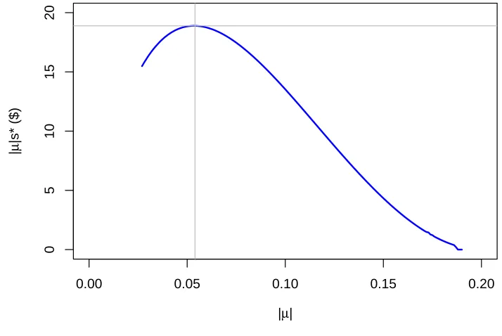
Within our interval of interest |µ| ∈[1

37,0.19], the optimal first-round side-bet stake is

mono-tonically decreasing in the absolute value of the operator’s mean return ∂s∗1µ

∂|µ| < 0, ∂2

s∗ 1µ

∂|µ|2 > 0.

But the product|µ|s∗

1µ does not inherit this property. We therefore ask whether the operator’s

expected payoff on the first-round side bet |µ|s∗1µreaches a maximum for some per-unit-bet

re-turn|µ|within the interval [₃₇1 ,0.19]. Figure 2 shows that this is indeed is the case, and that the

Un-der the assumptions and parameters of this working example, the per-unit-bet expected return

|µ|= 1

19 = 0.053 is within one-thousandth (0.001) of the optimal expected return |µˇ|= 0.054.

Figure 2: Expected payoff to gaming operator from the first-round side bet for different values of the|µ|parameter between|µ|= 1

37 = 0.027 and|µ

¯|= 0.19. Maximum occurs at (0.054,18.89).

0.00 0.05 0.10 0.15 0.20

0

5

10

15

20

|µ|

|

µ

|s* ($)

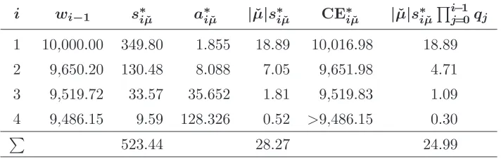
Table 3 shows that the operator’s first-round expected payoff |µˇ|s∗1 ˇµ = $18.89 under the

optimal expected return |µˇ|= 0.054 is a marginal improvement over the operator’s first-round

expected payoff |µ|s∗1µ = 18.86 under American-roulette expected return |µ|= 1

19. The

opera-tor’s sum of expected gross payoffs over the four individually EU-enhancing side-bet rounds is

$24.99, which compares favorably with $24.72 under|µ|= 1

19. Thus also in terms of the gaming

operator’s expected gross revenue, the optimal-expected-return case ˇµ=−0.054 dominates the

American-roulette expected return case µ = −1

19, but only marginally. In the present setting,

American roulette’s µ= −1

19 is a good practical approximation to the optimal ˇµ=−0.054.

4 Conclusion

In this note we revisit Bell’s (1988) finding that a pre-decision side bet can be a rational,

EU-enhancing strategy for determining whether to take on a large, indivisible, risky prospect.

Providers of side-bet services – gaming operators such as casinos and betting shops – do so on

an actuarially unfair basis. When pre-decision side bets are constrained to be actuarially unfair,

Table 3: Parameters of individually optimal EU-augmenting round-iside bets which maximize the gaming operator’s sum of expected payoffs (ˇµ=−0.054).

i wi−1 s∗iµˇ a∗iµˇ |µˇ|s∗iµˇ CE∗iµˇ |µˇ|s∗iµˇ Qi−1

j=0qj

1 10,000.00 349.80 1.855 18.89 10,016.98 18.89

2 9,650.20 130.48 8.088 7.05 9,651.98 4.71

3 9,519.72 33.57 35.652 1.81 9,519.83 1.09

4 9,486.15 9.59 128.326 0.52 >9,486.15 0.30 P

523.44 28.27 24.99

maker’s wealth consequently remains within the interval of interim convexity, instead of being

ejected to its lower boundary. Hence, the decision maker rationally engages in a further

side-bet round. Under the assumptions of Bell’s (1988) example, we find that the decision maker

rationally engages in up to four side-bet rounds (in one case, six rounds). For each successive

optimal side bet, the stake becomes smaller and the required odds become longer. This

ever-longer-odds requirement may hinder implementation of extended side-bet sequences in practice.

Nevertheless side-bet sequences are surprisingly general from a theoretical standpoint, as they

arise in all families of non-linear, non-exponential risk-averse utility functions. Together with

Bell’s (1988) seminal result, the present finding expands the range of empirical phenomena that

can be explained within the framework of normative rationality. However, it also introduces

a further set of methodological considerations that must be confronted in the design of

risk-aversion-elicitation procedures and in the empirical estimation of risk-aversion coefficients.

References

Bell, D. E. 1988. The value of pre-decision side bets for utility maximizers.Management Science

34_{(6) 797–800.}

Delqui´e, P. 2008. The value of information and intensity of preference. Decision Analysis 5₍₃₎

129–139.

Friedman, M., Savage, L. J. 1948. The utility analysis of choices involving risk. Journal of

Political Economy 56_{(4) 279–304.}

Raiffa, H. 1968. Decision Analysis. Reading, MA: Addison-Wesley.

A Side-bet bounds

The tangent line tou(·) at (w0′, u(w′0)), whereu(w0) = ln(w0), is

y = u(w0′) +u′(w0′)(w0−w′0) (9)

= ln(w0′) +

w0−w0′

w′0

(10)

while the tangent line tov(·) at (w′′0, v(w0′′)), wherev(w0) = 1₂ln(w0+ 10,000)+1₂ln(w0−5,000),

is given by

y = u(w0′′) +u′(w′′0)(w0−w′′0) (11)

= 1 2

ln(w0′′+ 10,000) + ln(w′′0−5,000) +

w0−w′′0

w′′

0+ 10,000

+ w0−w

′′

0

w′′

0 −5,000

. (12)

In order for these lines to be the same (i.e. a common tangent tou(·) and v(·)) then they must

share the same slope

1

w′

0

= 1

2(w′′

0 + 10,000)

+ 1

2(w′′

0 −5,000)

(13)

and vertical intercept

ln(w0′)−1 =

1 2

ln(w0′′+ 10,000) + ln(w′′0−5,000)−

w′′0

w′′

0+ 10,000

− w

′′

0

w′′

0 −5,000

. (14)

Solving these two equations computationally yields (w′