OPTIMAL PLACEMENT OF PILES IN REAL GRILLAGES:
EXPERIMENTAL COMPARISON OF OPTIMIZATION ALGORITHMS
Rimantas Belevi
č
ius
*, Serg
ė
jus Ivanikovas
**, Dmitrij Šešok
*,***,
Saulius Valentinavi
č
ius
*, Julius Žilinskas
***,**Vilnius Gediminas Technical University, Vilnius, Lithuania **Vilnius Pedagogical University, Vilnius, Lithuania
***Institute of Mathematics and Informatics, Vilnius University, Akademijos 4, Vilnius, Lithuania
e-mail: [email protected], [email protected]
Abstract. The aim of the article is to choose algorithms suited for optimal placement of piles in real grillages by performing experimental comparison of different global optimization algorithms. The comparison includes several algorithms: random search, metaheuristics (simulated annealing and genetic algorithm) and local optimization com-bined with random search. The algorithms are compared using the results of optimization of pile placement schemes of 10 practical grillages of small-to-medium scale with data obtained from several design bureaus. The best results have been achieved with simulated annealing and nonlinear optimization algorithm NEWUOA combined with heuristic random search.
Keywords: global optimization, metaheuristics, optimal design of grillage-type foundations.
1. Introduction
Finding a global optimum in industrial optimiza-tion problems usually is a difficult and time-con-suming task. A number of studies are published comparing various optimization algorithms. A fre-quent pitfall with comparative studies of this type is a difficulty to generalize the results to other problems. Each search method has its own characteristics which make the various search techniques more suited to different problem domains. Eriksson and Arora (2002) presented a comparison of global optimization algo-rithms applied to industrial ride comfort optimization problem. The genetic algorithm (GA) was found more efficient than the simulated annealing (SA) algorithm for this particular problem. Dumas et al. (2005) studied the drag reduction in the automotive industry problem. Various modifications of GAs were com-pared; in the most successful case the computational time of a GA is reduced by a factor up to 7. Fowler et al. (2008) compare the derivative-free optimization methods for groundwater supply problems. Horne and MacBeth (1998) applied global optimization algo-rithms to the problem of geophysical inversion and did not find pronounced advances of Tabu Search, GA and SA for this problem.
In this paper we shall concentrate on one specific class of optimization problems in civil engineering – optimal design of grillage-type foundations, which are called “grillages” throughout this paper. Grillages are
the most popular and effective scheme of foundations, especially in the case of weak grounds. The grillages consist of supporting piles and connecting beams. Bowles (1996), Reese et al. (2005) outline exhaustive technical details on the grillages. However, only a few works so far deal with optimization of foundation schemes. Chan et al. (2009) combine the sizing and topology optimization, however the piles are aggre-gated to special groups. Kim et al. (2001) minimize the differential settlements of piled rafts, again, by a special way minimizing the number of design va-riables. We are trying to obtain the globally minimal price of pile foundations treating all piles as a separate design variables. Belevičius and Valentinavi-čius (2001) and Belevičius et al. (2002) introduced the idealizations of real grillages, which are taken in the present mathematical model as well.
The optimal grillage should meet twofold criteria: the number of piles should be minimal, and connec-ting beams should receive minimal possible torques. In fact, here we encounter two separate optimization problems: search for the minimal number of piles and search for the minimal volume of beams. Both prob-lems can be integrated into one with a compromise objective function. We assume that the characteristics of piles and connecting beams are given and consider the first optimization problem.
Initial data for the grillage optimization problem are the following:
The geometrical scheme of connecting beams;
Cross-section data of all beams (area, moments of inertia);
Material data of all beams (material in one beam is treated as isotropic);
Positions of immovable piles (if any);
Maximum allowable reactive force at any pile;
Minimum possible distance between adjacent piles;
Vertical and two rotational stiffnesses (along the beam and normal to the beam) of pile;
Loading data. Active forces can be applied in the form of concentrated loads and moments at any point on beam, or in the form of distributed trapezoidal loadings at any segment of beam. The results of optimization are the number of re-quired piles and their positions. To solve this problem it is necessary to find such a placement of the given number of piles that reactive forces do not exceed the carrying capacities of piles. If such a placement is not possible, the number of piles should be increased.
Therefore we formulate a problem of placement of piles searching for appropriate pile positions under connecting beams. In an ideal grillage, reactive forces at all piles are identical. Practically this is hardly feasible, particularly when a designer introduces the so-called “immovable supports” that have to retain their positions and cannot change them during optimization process. Some technological constraints may also make the ideal scheme non-achievable, for example, the distance between adjacent piles cannot be too small due to the specific capacities of a pile driver. In the present work we do not consider the immovable supports and allow for a pile to take whatever position in the grillage, thus typically the piles are not placed at the joints of grillage. This fact confines the pile placement problem scope to a low-rise buildings without significant overturning mo-ments due to horizontal thrust, e.g. due to earthquake loading or wind loads.
The objective function for minimization can be formulated in several alternative forms, e.g. the maxi-mal vertical reactive force at a pile, the difference between the maximal and minimal reactive forces in the whole grillage, or the maximal difference between the reactive force and carrying capacity of a pile. A grillage supported by piles with different character-ristics can be optimized using the third objective func-tion menfunc-tioned. We assume that the characteristics of all piles are equal and in this case the first and last objective functions are equivalent. We use the first objective function in the current paper.
An even distribution of reactive forces or differ-rences between reactions and carrying capacities among all piles indicates an ideal grillage. Therefore the ideal value of the objective function or the lower bound for the minimum is known in advance. This makes the problems attractive as test sets for expe-rimental investigation of optimization algorithms
since it can be estimated how far the best value found is from the ideal one.
Our experience shows that the objective function for practical grillage optimization problems possesses many local minima points. Another complicated trait of the problem is that usually the objective function is very sensitive to the positions of piles: sometimes even a small alteration of one position leads to a sig-nificant change of the value of the objective function. All this makes the placement of piles in practical grillage a difficult global optimization problem.
In our previous work we tried to approach the problem as “black-box” global optimization by cove-ring methods (Čiegis et al. 2006; Žilinskas 2008), genetic algorithms (Belevičius and Šešok 2008), and local optimization combined with random search (Iva-nikovas et al. 2009), but the results were not inspiring even for problems with 10 and 15 piles. One possible reason is that heuristic information on the problem is not employed in the case of “black-box” optimization. In this paper we compare different strategies for solution of the problem: starting from random search and heuristic random search, then progressing to meta-heuristics (simulated annealing and genetic algo-rithms) and local optimization combined with heu-ristic random search. Promising results have been achieved when heuristic random search is combined with metaheuristics and local optimization.
The algorithms are compared using the results of optimization of pile placement schemes of 10 practical grillages. All these grillages are of small-to-medium scale, requiring from 18 to 55 piles. Data for these problems are obtained from several Dutch design bureaus (courtesy of Consultancy W.F.O. B.V., Paauw B.V. Aannemingsbedrijf, Aannemingsbedrijf V. Dijk, Bouwtectuur West Friesland, Stabo Bouw B.V., Aan-nemingsbedrijf A. Tuin Den Helder and others) which use the professional software for structural enginee-ring package MatrixFrame ( http://www.matrix-soft-ware.com/uk/structuralengineering/matrixframe/ index.html). It is intended for an analysis and design of steel and concrete erections. Apropos, MatrixFrame
implemented our software for optimization of pile placement schemes employing local search methods (Belevičius and Valentinavičius 2001). However, the current optimization routine of MatrixFrame was not capable to yield even a rational scheme of pile place-ment for the problems considered in this paper.
2. Mathematical formulation
The optimization problem is formulated as follows: )
x ( min *
D x f f
,
where is a nonlinear objective function of con-tinuous variables , represent design parameters defining positions of piles, their number is denoted by n, is a feasible region. Besides of
) x ( f
n
f :
n
x
the global minimum , one or all global minimizers should be found. No assumptions on unimodality are included into formulation of the problem – many local minima may exist.
* f ) x ( i 1 p * *) x ( : *
x f f
max ) x ( , , 1 N i f p N 0 i
In this paper the maximal vertical reactive force at a pile is considered as the objective function:
R
p
,
where is the number of piles, is the reactive force at the i-th pile.
) x (
i R
Since a supporting pile may reside only under con-necting beams, there are evident restrictions on the positions of piles: during the optimization process the piles can move only along the connecting beams. Therefore, a two-dimensional beam structure of the grillage is “unfolded” to a one-dimensional construct, and the piles are allowed to range through this space freely.
Unfortunately in such a formulation small varia-tion of the design variable may correspond to a finite variation of the position of the pile in the physical space, what leads to discontinuity of the problem. One possibility to overcome this is to use multilevel opti-mization where the upper level combinatorial problem assigns piles to beams, while the lower level con-tinuous problems aim to position the piles in the assigned beams. Another possibility is to divide search space avoiding jumps of piles from one beam to ano-ther and perform searches in such separate spaces. However both possibilities are applicable only when a considerable number of objective function evaluations can be performed. Since evaluation of objective func-tion of pile placement based on finite element analysis is computationally expensive and we will perform only 5000 evaluations in each run of optimization algorithm, we do not think these possibilities are ap-plicable. Unfortunately, we do not know a parameter-rization that would not introduce discontinuities and lead to simpler optimization problem.
One design parameter corresponds to a position of one pile in the one-dimensional construct. The back-ward transformation restores the positions of piles in the two-dimensional beam structure of the grillage. The constraints for the design parameters are as follows:
x L, i
i
,...,N ,
where
x
is a design parameter defining the position of the i-th pile, L is the total length of all beams in the grillage. If the minimal possible distance between adjacent piles is specified, there are additional const-raintsj i , j
ix
x ,
where are two-dimensional coordinates of piles and
i
x
j ix
x denotes the distance between piles. To cope with this constraint, a penalty is included in the
objective function.
A finite element program is used as a “black-box” routine to the optimization program for solution of direct problem to find reactive forces in the grillage. In the direct problem that is solved via finite element analysis, the connecting beams in the grillage are idealized as the beam elements, while the piles are treated as supports, i.e. finite element mesh nodes with given elastic boundary conditions. Since time of opti-mization crucially depends on time of solution the direct problem, fast problem-oriented original FORTRAN programs with a special mesh pre-processor have been developed and used.
The beam elements have 2 nodes with 6 degrees of freedom each (3 displacements along the coordinate axes and 3 rotations about these axes). The stiffness matrix for element can be found in many textbooks, e.g. by Spyrakos and Raftoyiannis (1997):
22 12 12 11 K K K KK T ,
L EI 4 L EI 6 0 L EI 4 L EI 6 0 L GJ 0 L EI 6 L EI 12 0 L EI 6 L EI 12 0 0 0 0 0 0 L EA z 2z y 2 y 2 y 3 y 2z 3z 11 K , L EI 2 L EI 6 0 L EI 2 L EI 6 0 L GJ 0 L EI 6 L EI 12 0 L EI 6 L EI 12 0 0 0 0 0 0 L EA z 2 z y 2 y 2 y 3 y 2 z 3 z 12 K ,where E is the Young‘s modulus, A is a cross-sectional area of the beam, J, Izand Iy are the inertial moments
of cross-section. Sub-matrix [K22] coincides with [K11]
but non-diagonal members are with opposite signs. The main statics equation is
a
a
a F uK ,
where a stands for the ensemble of elements (not shown in eq. below), {u} are the nodal displacements, and {F} are the active forces. The reactive forces at piles are available after obtaining the nodal displace-ments:
j j iji K u
R .
3. Optimization algorithms
Several algorithms have been employed for place-ment of piles minimizing the maximal vertical reactive force at a pile:
Random search (RS);
Modified random search (MRS);
Simulated annealing (SA);
Genetic algorithm (GA);
Simplex method (SM);
Variable metric method (VM);
NEWUOA algorithm.
To make a fair comparison, the total number of objective function evaluations for each algorithm is the same: N=5000. The values for parameters of the algorithms have been chosen according to the results of exhaustive numerical investigation.
Random search is performed generating decision variables randomly with uniform distribution. N inde-pendent random structures are generated and reactive forces at the piles are found using finite element ana-lysis. The structure with the smallest maximal reactive force at a pile is considered to be the best solution found.
Heuristic information is employed in modified random search. Decision variables are generated ran-domly with uniform distribution, but additional const-raint is set: the difference of two decision variables should be larger than S which is obtained by dividing the half of the total length of all beams by the number of piles:
p j
i x S i j S NL x
2 ,
,
.
The value of decision variable is regenerated ran-domly with uniform distribution if it is too close to a value of a previously generated decision variable. Such a heuristic modification is motivated by the fact that due to the usual distribution of loading over the grillage beams, the piles also should be spread over the whole space of grillage. Reactive forces at the piles are found for N feasible random structures and one with the smallest maximal reactive force at a pile is considered to be the best solution found.
Simulated annealing (Kirkpatrick et al. 1983) replaces the current solution by a random solution with a probability that depends on the difference of the function values and a temperature parameter. In the beginning the temperature parameter is large allowing non-improving changes. Gradually temperature is de-creased and the search becomes descent. In our imple-mentation the initial solution is obtained using RS or MRS taking the best feasible solution out of
N_init=200. Then SA algorithm is employed. A new potential set of values of decision variables is found adding independent random numbers uniformly distributed over [-y, y] to the current values. The value of y is gradually reduced during the solution process: in the iterations from 201 to (2N/5) it is equal to 0.5,
in the succeeding (2N/5) iterations – 0.1, and in the final N/5 iterations – 0.05. All these values are chosen on the basis of numerical experiments. If the value of the objective function with the set of new values of decision variables is better than the previous one, the values of decision variables values are modified with probability 1; otherwise – with probability
t j t
h
e
2
1/ln1 ,
where h denotes the difference between the best so far value of the objective function and its value after modification, t1 is the initial temperature, t2 is the
annealing speed, and j denotes the iteration number. The SA algorithm proceeds until j exceeds the given number of iterations N.
Genetic algorithms (Goldberg 1989) simulate evo-lution (selection, mutation, crossover) in which a po-pulation of solutions evolves improving values of the objective function. In our implementation, the initial population of popsize individuals is generated using RS or MRS. The new generation is obtained from the previous one using selection, crossover and mutation operations. During the selection, popsize/2 pairs of in-dividuals are selected for breeding by the roulette principle. The individuals with a better objective func-tion value have higher probability to be selected. The probability that the j-th individual with an objective function value fj will be chosen is
i i j j
f f
p 1 1 ,
where the sum operator covers entire population. The crossover between two individuals chosen for bree-ding is performed with probability p_cross; the cross-over position is obtained randomly from the interval of [1, Na-1]. The mutation is performed with
probability p_mut to each decision variable: the value is augmented by a random number uniformly distri-buted over [-y, y]. The algorithm proceeds for the given number of generations (G). As in SA, the value of y is gradually reduced in the same manner: y = 0.5 for the generations 2nd to the (2G/5), y = 0.1 for the
generations (2G/5+1) to (4G/5), and y = 0.05 for the last G/5 iterations.
The simplex method proceeds while the overall number of objective function evaluations reaches N.
Variable metric methods (also known as quasi-Newton methods) are based on quasi-Newton’s method to find the stationary point of the objective function where the gradient is 0. However Hessian matrix does not need to be computed, but it is updated by analy-zing successive gradient vectors. We use implement-tation of Broyden-Fletcher-Goldfarb-Shanno (BFGS) method from Press (1992). Since variable metric method requires gradient information, the results of sensitivity analysis are used. The starting point is the best solution obtained using RS or MRS in the given number of iterations N_init. Then local optimization is performed. Initialization and local search is repeated until the overall number of function evaluations reaches N. Evaluations of objective function and gra-dient (sensitivity analysis) function are counted, com-putational time of these two functions is not very different.
The NEWUOA algorithm is an iterative algorithm for nonlinear optimization. A quadratic model is used in a trust region procedure for adjusting the variables (Powell 2006). The quadratic model interpolates the function at 2n+1 points, only one interpolation point is altered on each iteration. The starting point is the best solution obtained using RS or MRS in the given number of iterations N_init. The NEWUOA algorithm is stopped when the number of objective function evaluations reaches N.
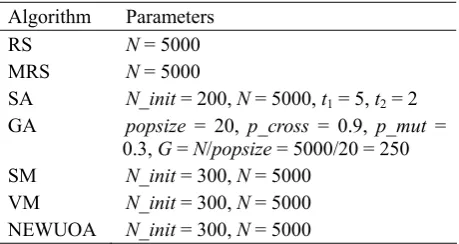
The values of main parameters of the algorithms are summarized in Table 1. Other parameters, for example the initial temperature for SA or probabilities of crossover and mutation for GA are tuned to the problems under consideration.
Table 1. Parameters for algorithms
Algorithm Parameters RS N = 5000 MRS N = 5000
SA N_init = 200, N = 5000, t1 = 5, t2 = 2
GA popsize = 20, p_cross = 0.9, p_mut = 0.3, G = N/popsize = 5000/20 = 250 SM N_init = 300, N = 5000
VM N_init = 300, N = 5000 NEWUOA N_init = 300, N = 5000
4. Numerical examples and timings
The characteristics of test problems are presented in Table 2. There are no immovable piles, therefore the numbers of piles (Np) and decision variables (n)
coincide. Rallw denotes the allowable reactive force at
the piles. In all problems it is equal for all piles of grillage. The number of piles is obtained by dividing the sum of loadings by the allowable reactive force of piles – the number of piles cannot be less than this number. Rideal denotes the ideal theoretical value. The
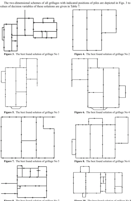
ideal solution is when all reactive forces at the piles are equal. In this case the reactive forces are equal to the sum of loadings divided by the number of piles. In all these problems the proportion between the total loading and the allowable reaction is such that the engineering solution requires achieving almost the ideal solution. This is the main reason, why these problems are difficult to solve. The typical grillage together with obtained pile positions is shown in Figu-re 1. The two-dimensional schemes of all grillages with indicated positions of piles are depicted in Figures 3 to 12 in Appendix.
Table 2. Characteristics of problems
Problem No Np L Rallw Rideal
1 25 172.90 325 307.47
2 18 52.90 110 104.12
3 31 84.10 105 101.85
4 31 84.90 105 101.24
5 30 63.90 100 97.51
6 37 80.10 100 97.53
7 23 129.10 300 287.35
8 34 137.90 250 236.28
9 17 97.60 250 244.71
10 55 315.61 350 349.05
Figure 1. Grillage No 1 (according to Table 2)
The black-box finite element routine for evaluation of the objective function in a library format together with 10 grillage data (txt format) and FORTRAN example file are available at: http://soften.ktu.lt/ ~mockus/grillage/contgrillage.html.
achieved by SA and NEWUOA. Results of GA are close, while RS, MRS, SM and VM perform worse. When MRS is used for initialization NEWUOA signi-ficantly outruns SA for Problem 8 (34 piles). It shows slightly better results also for Problems 4 (31) and 6 (37). Nearly in all cases the GA shows the third best solutions; it never outruns the SA or NEWUOA algo-rithms. The results of SM and VM are sometimes even worse than that of MRS what means that it is not worth to spend time to find local minima for these problems, but rather to search wider globally since lo-cal searches do not improve the value of the objective function significantly. Good performance of SA and GA does not surprise since their parameters (for example the initial temperature for SA or probabilities of crossover and mutation for GA) are tuned to the problems under consideration. NEWUOA optimizes a quadratic model of the objective function and per-forms better than local optimization of the objective function itself. The use of a model allows overcoming of problems of discontinuity and non-differentiability.
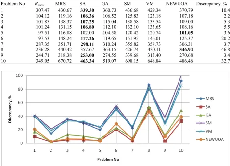
The best obtained results in 28 runs are rendered in Table 5. MRS is used for initialization. NEWUOA obtains the best solutions for two problems, for other problems SA provides better results. An ideal solution was not obtained for any problem in any of 28 inde-pendent runs; in each run the objective function was evaluated 5000 times. The best values found in 28 runs normalized to Rideal (discrepancies in %) are
shown in Figure 2. The last column of Table 5 pre-sents discrepancies between the best obtained results and the corresponding ideal value. The best objective values found differ from ideal from 2.2% (Problem 2, 18 piles) to 46.8% (Problem 8, 34 piles). As it can be expected, generally discrepancy is larger for problems with the larger number of piles. Thus, for Problem 8 (34 supports), 10 (55), and 6 (37) the discrepancies between the best obtained and ideal values are respectively 46.8%, 32.7%, and 20.2%, while for Problems 2 (18), 9 (17), and 5 (30) – 2.2%, 3.4%, and 3.6%. Also, the character of loading distribution over the grillage plays a crucial role too.
Table 3. Average of the best values found in 28 runs when RS is used for search and initialization
Problem No Rideal RS SA GA SM VM NEWUOA
1 307.47 593.33 463.08 490.01 633.77 547.63 440.31
2 104.12 153.07 119.74 119.60 172.79 152.38 118.68
3 101.85 258.45 134.59 142.24 274.06 230.73 139.88
4 101.24 265.41 139.63 149.87 264.42 251.90 136.43
5 97.51 318.16 132.52 142.53 310.40 290.67 128.79
6 97.53 460.31 162.09 175.90 460.16 435.57 188.60
7 287.35 472.74 372.63 380.48 507.99 450.81 369.03
8 236.28 695.60 455.63 479.87 721.70 655.56 467.22
9 244.71 402.17 307.55 321.27 427.50 385.72 296.27
10 349.05 1321.48 806.46 890.51 1319.49 1163.32 771.26
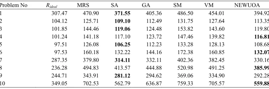
Table 4. Average of the best values found in 28 runs when MRS is used for search and initialization
Problem No Rideal MRS SA GA SM VM NEWUOA
1 307.47 470.90 371.55 405.36 486.50 454.01 394.92
2 104.12 125.71 109.10 112.49 131.75 127.64 113.35
3 101.85 144.46 119.06 124.48 153.82 143.60 119.80
4 101.24 141.18 117.10 123.72 147.46 139.82 116.81
5 97.51 126.08 106.25 112.23 133.28 128.13 108.68
6 97.53 160.18 132.22 144.16 172.38 160.85 132.07
7 287.35 379.80 314.11 332.11 402.36 382.45 330.16
8 236.28 494.83 413.57 444.88 520.98 491.25 385.99
9 244.71 343.91 281.12 294.62 369.06 334.90 292.28
10 349.05 702.53 562.79 636.87 759.33 705.57 559.88
Average times of one run in seconds are shown in Table 6. One numerical experiment takes from appro-ximately 1.5 (algorithm GA, Problem 2, 18 piles) to 41 minutes (SM, Problem 8, 34 piles). Peculiarly, the more complex-looking grillages 10 (55 supports) and 6 (37) take shorter time for almost all algorithms. The related question is, why in several cases RS takes lon-ger time than, e.g., MRS or GA that employ additional
render more even distribution of supports which re- sults in a lesser finite element mesh.
Table 5. The best values found in 28 runs
Problem No Rideal MRS SA GA SM VM NEWUOA Discrepancy, %
1 307.47 430.67 339.30 360.73 436.68 429.34 370.79 10.4
2 104.12 119.16 106.36 106.52 125.83 123.18 107.18 2.2
3 101.85 138.37 107.25 115.04 138.58 135.54 109.00 5.3
4 101.24 131.15 106.80 112.10 132.10 133.65 108.16 5.5
5 97.51 116.88 102.00 104.58 120.42 120.74 101.05 3.6
6 97.53 148.24 117.26 119.65 151.95 146.01 125.37 20.2
7 287.35 351.71 298.11 310.24 355.82 358.73 306.31 3.7
8 236.28 440.42 357.67 363.15 426.74 430.11 346.94 46.8
9 244.71 318.38 253.00 274.55 339.68 313.40 270.68 3.4
10 349.05 670.72 463.34 519.07 698.15 648.84 486.46 32.7
Figure 2. The best values found in 28 runs normalized to Rideal (discrepancies in %) Table 6. Average times of one run, sec
Problem No Na RS MRS SA GA SM VM NEWUOA
1 25 899 943 960 844 821 855 878
2 18 92 96 91 82 90 91 91
3 31 835 876 822 732 811 801 753
4 31 1015 1045 1046 935 910 914 916
5 30 319 319 302 276 313 318 315
6 37 811 823 742 718 674 761 750
7 23 649 695 683 635 622 660 656
8 34 3009 2982 2956 2668 2467 2455 2489
9 17 424 417 410 359 413 419 423
10 55 2198 2136 2125 1934 1826 1811 1850
Comparing the timings of all algorithms, the clear winners here are the GA and SM. However, the other algorithms are not far behind, until ~18% in ultimate cases. Thus, the timings cannot be treated as the deci-sive factor for comparison of these algorithms. This is due to the fact that most of the time is spent for eva-luation of the objective function. In such cases it is worth to use optimization algorithms with more auxi-liary computations, as NEWUOA is. Although
auxilia-ry computations improve the results, optimization time is still quite similar.
5. Conclusions
the engineering purposes. The simulated annealing, genetic algorithm and nonlinear optimization algo-rithm NEWUOA applied from a good random point can be successfully used to obtain rational pile placement schemes under the small- and moderate-scale grillages.
The results of simplex and variable metric methods show that the problems of pile placement have a number of local minima and it is not worth to spend time to find local minima for these problems, but ra-ther to search wider globally. This is why simulated annealing and genetic algorithm perform better for these problems. NEWUOA optimizes a quadratic model of the objective function and performs better than local optimization of the objective function itself. Evaluation of objective function of pile placement based on finite element analysis is computationally expensive. Because of this, timings of all algorithms are quite similar when stopping condition is the num-ber of function evaluations. Therefore timings cannot be treated as the decisive factor for application of the algorithms to this problem. In such cases the use of optimization algorithms with more auxiliary computa-tions is worth as can be seen from good results of NEWUOA – auxiliary computations improve the results, but do not prolong optimization time con-siderably.
Several runs of the algorithm are necessary to find good solutions. Inclusion into the algorithm even some information about the problem (due to the usual distribution of loading over the grillage beams, the piles also should be spread over the whole space of grillage) significantly improves the results – this is general to all algorithms tested.
Acknowledgements
This work was supported by the Lithuanian State Science and Studies Foundation within the project B-03/2007 “Global optimization of complex systems using high performance computing and grid tech-nologies”. The work of the third author was also par-tially supported by the Research Council of Lithuania (contract No MOS-10/2010 “Use of stochastic global optimization methods in engineering”).
References
[1] R. Belevičius, D. Šešok. Global optimization of gril-lages using genetic algorithms. Mechanika 6(74), 2008, 38-44.
[2] R. Belevičius, S. Valentinavičius. Optimisation of grillage-type foundations. In: Proceedings of 2nd Eu-ropean ECCOMAS and IACM Conference “Solids, Structures and Coupled Problems in Engineering”, Cracow, Poland 26-29 June, 2001.
[3] R. Belevičius, S. Valentinavičius, E. Michnevič. Multilevel optimization of grillages. Journal of Civil Engineering and Management 8(2), 2002, 98-103 [4] J.E. Bowles. Foundation Analysis and Design. 5thed.
McGraw-Hill, 1996.
[5] C.M. Chan, L.M. Zhang, J.T.M. Ng. Optimization of pile groups using hybrid genetic algorithms.
Jour-nal of Geotechnical and Geoenvironmental Enginee-ring 135(4), 2009, 497-505.
[6] R. Čiegis, M. Baravykaitė, R. Belevičius. Parallel global optimization of foundation schemes in civil engineering. Lecture Notes in Computer Science 3732, 2006, 305-313.
[7] L. Dumas, V. Herbert, F. Muyl. Comparison of global optimization methods for drag reduction in the automotive industry. Lecture Notes in Computer Science 3483, 2005, 948-957.
[8] P. Eriksson, J.S. Arora. A comparison of global opti-mization algorithms applied to a ride comfort optimi-zation problem. Structural and Multidisciplinary Optimization 24(2), 2002, 157-167.
[9] K.R. Fowler, J.P. Reese, C.E. Kees, J.E. Dennis Jr., C.T. Kelley, C.T. Miller, C. Audet, A.J. Booker, G. Couture, R.W. Darwin, M.W. Farthing, D.E. Fin-kel, J.M. Gablonsky, G. Gray, T.G. Kolda. Com-parison of derivative-free optimization methods for groundwater supply and hydraulic capture community problems. Advances in Water Resources 31(5), 2008, 743-757.
[10] D.E. Goldberg. Genetic Algorithms in Search, Opti-mization and Machine Learning. Addison-Wesley, New York, 1989.
[11] S. Horne, C. MacBeth. A comparison of global opti-misation methods for near-offset VSP inversion. Com-puters & Geosciences 24(6), 1998, 563-572.
[12] S. Ivanikovas, E. Filatovas, J. Žilinskas. Experi-mental investigation of local searches for optimization of grillage-type foundations. In: Čiegis R, Henty D, Kågström B, Žilinskas J (eds) Parallel Scientific Com-puting and Optimization. Vol. 27 of Springer Optimi-zation and Its Applications, Springer, 2009, 103-112. doi:10.1007/978-0-387-09707-7_9.
[13] K.N. Kim, S.-H. Lee, K.-S. Kim, C.-K. Chung, M.M. Kim, H.S. Lee. Optimal pile arrangement for minimizing differential settlements in piled raft foundations. Computers and Geotechnics 28(4), 2001, 235-253.
[14] S. Kirkpatrick, C.D.J. Gelatt, M.P. Vecchi. Optimi-zation by simulated annealing. Science 220(4598), 1983, 671-680.
[15] J.A. Nelder, R. Mead. A simplex method for function minimization. The Computer Journal 7(4), 1965, 308-313.
[16] M.J.D. Powell. The NEWUOA software for unconst-rained optimization without derivatives. In: Di Pillo G, Roma M (eds) Large-Scale Nonlinear Optimi-zation. Vol. 83 of Nonconvex Optimization and Its Applications, Springer, 2006, 255-296.
[17] L.C. Reese, W.M. Isenhower, S.-T. Wang. Analysis and Design of Shallow and Deep Foundations. John Wiley & Sons, 2006.
[18] C. Spyrakos, J. Raftoyiannis. Linear and Nonlinear Finite Element Analysis in Engineering Practice. Al-gor Publishing Division, 1997.
[19] W.H. Press. Numerical Recipes in Fortran 77: The Art of Scientific Computing. 2nd edn. Cambridge Uni-versity Press, 1992.
Appendix: Solutions of the problems
The two-dimensional schemes of all grillages with indicated positions of piles are depicted in Figs. 3 to 12. The values of decision variables of these solutions are given in Table 7.
Figure 3. The best found solution of grillage No 1 Figure 4. The best found solution of grillage No 2
Figure 5. The best found solution of grillage No 3 Figure 6. The best found solution of grillage No 4
Figure 7. The best found solution of grillage No 5 Figure 8. The best found solution of grillage No 6
Figure 11. The best found solution of grillage No 9 Figure 12. The best found solution of grillage No 10
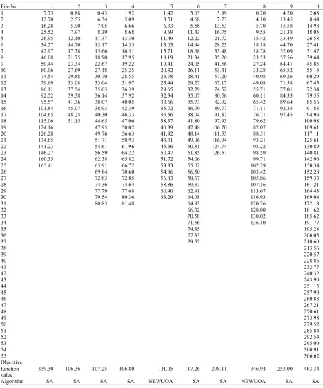
Table 7. The best found solutions: values of decision variables in one-dimensional construct of grillage (with an accuracy of 1 cm)
Pile No 1 2 3 4 5 6 7 8 9 10
1 7.75 0.88 0.43 1.92 1.42 3.05 3.99 0.20 4.20 2.68
2 12.70 2.55 6.34 5.09 3.51 4.68 7.73 4.10 13.45 8.44
3 16.28 5.90 7.05 6.66 6.33 5.58 13.53 5.70 15.58 14.98 4 25.52 7.97 8.39 8.68 9.69 11.43 16.75 9.55 21.38 18.05 5 26.95 12.10 11.37 13.30 11.49 12.22 21.72 15.42 33.49 26.58 6 34.27 14.70 13.17 14.55 13.03 14.94 28.23 18.18 44.70 27.41 7 42.97 17.38 15.66 16.51 15.71 18.68 33.48 18.78 52.09 31.47 8 46.08 21.75 18.90 17.95 18.19 21.34 35.26 23.53 57.56 39.64 9 50.44 23.34 22.67 19.22 19.41 24.05 41.56 27.24 64.41 45.85 10 60.06 27.69 27.18 25.25 20.32 26.11 53.41 33.28 65.52 55.15 11 74.54 29.88 30.70 28.55 23.78 28.41 57.20 40.98 69.26 60.29 12 79.69 33.08 33.04 31.97 25.44 29.27 67.17 49.08 71.58 67.45 13 86.11 37.54 35.03 36.39 29.65 32.29 74.52 55.71 77.01 72.34 14 92.52 39.38 36.14 37.92 32.34 35.07 80.56 60.11 84.33 79.55 15 95.57 41.36 38.07 40.05 33.66 35.73 82.92 65.42 89.64 85.56 16 101.84 45.07 38.93 42.39 35.72 36.79 89.77 71.11 92.35 91.83 17 104.65 48.25 40.30 46.33 36.56 38.04 91.87 76.71 97.45 94.96 18 115.06 51.15 44.65 47.06 38.37 41.80 97.93 79.62 100.98 19 124.16 47.95 50.02 40.39 47.48 106.70 82.07 109.61 20 126.28 49.76 56.63 41.92 48.14 111.53 88.51 117.11 21 134.85 51.71 58.93 43.31 49.06 116.94 93.21 125.61 22 141.23 54.61 61.96 45.36 50.81 124.74 95.22 130.89 23 146.27 56.59 64.22 50.47 51.85 126.57 98.59 140.81
24 160.35 62.38 65.82 51.72 54.06 99.71 142.96
25 165.41 65.91 66.72 53.33 55.02 102.29 150.34
26 69.84 70.60 54.86 56.50 103.42 152.28
27 72.83 72.85 56.83 58.67 105.86 159.33
28 74.36 74.64 58.86 59.37 107.16 161.21
29 77.79 77.68 60.40 62.91 113.67 164.43
30 79.54 80.36 63.29 64.08 116.93 169.04
31 80.83 81.48 64.93 120.26 172.18
32 66.32 128.00 181.62
33 70.58 130.02 185.62
34 71.56 136.10 191.77
35 74.35 195.28
36 77.33 206.05
37 79.57 210.60
38 213.56
39 220.57
40 228.86
41 232.77
42 240.32
43 243.90
44 251.15
45 257.90
46 260.88
47 267.21
48 270.61
49 275.98
50 279.52
51 285.84
52 292.54
53 295.00
54 300.91
55 306.62
Objective function
value 339.30 106.36 107.25 106.80 101.05 117.26 298.11 346.94 253.00 463.34
Algorithm SA SA SA SA NEWUOA SA SA NEWUOA SA SA