Enhanced processing in arrays of optimally tuned nonlinear biomimetic sensors : a coupling mediated Ringelmann effect and its dynamical mitigation

warwick.ac.uk/lib-publications

Original citation:

Nikitin, Alexander P., Bulsara, Adi R. and Stocks, Nigel G.. (2017) Enhanced processing in

arrays of optimally tuned nonlinear biomimetic sensors : a coupling-mediated Ringelmann

effect and its dynamical mitigation. Physical Review E (Statistical, Nonlinear, and Soft Matter

Physics), 95 (3). 032211.

Permanent WRAP URL:

http://wrap.warwick.ac.uk/87492

Copyright and reuse:

The Warwick Research Archive Portal (WRAP) makes this work by researchers of the

University of Warwick available open access under the following conditions. Copyright ©

and all moral rights to the version of the paper presented here belong to the individual

author(s) and/or other copyright owners. To the extent reasonable and practicable the

material made available in WRAP has been checked for eligibility before being made

available.

Copies of full items can be used for personal research or study, educational, or not-for-profit

purposes without prior permission or charge. Provided that the authors, title and full

bibliographic details are credited, a hyperlink and/or URL is given for the original metadata

page and the content is not changed in any way.

Publisher statement:

© 2017 American Physical Society

A note on versions:

The version presented here may differ from the published version or, version of record, if

you wish to cite this item you are advised to consult the publisher’s version. Please see the

‘permanent WRAP URL’ above for details on accessing the published version and note that

access may require a subscription.

Coupling-Mediated Ringelmann Effect and its Dynamical Mitigation

Alexander P. Nikitin,1,∗ _{Adi R. Bulsara,}2,† _{and Nigel G. Stocks}1,‡ 1

School of Engineering, University of Warwick, Coventry CV4 7AL, UK

2

Space and Naval Warfare Systems Center Pacific, Code 71000, San Diego, CA 92152-6147, USA (Dated: February 6, 2017)

Inspired by recent results on self-tunability in the outer hair cells of the mammalian cochlea, we describe an array of magnetic sensors where each individual sensor can self-tune to an optimal operating regime. The self-tuning gives the array its “biomimetic” features. We show that the overall performance of the array can, as expected, be improved by increasing the number of sensors but, however, coupling between sensors reduces the overall performance even though the individual sensors in the system could see an improvement. We quantify the similarity of this phenomenon to the Ringelmann Effect that was formulated 103 years ago to account for productivity losses in human and animal groups. We propose a global feedback scheme that can be used to greatly mitigate the performance degradation that would, normally, stem from the Ringelmann Effect.

PACS numbers: 05.40.-a, 07.55.Ge, 89.75.-k

I. INTRODUCTION

Biological sensory systems are remarkable in their abil-ity to detect extremely weak signals. As examples, the human eye is able to count single photons [1], hair cells in the cat cochlea are able to detect displacements of the basilar membrane smaller than 10−10 _{m [1], the} ol-factory system of the domesticated silk moth (Bombyx mori) can detect single molecules of pheromone [2], and thermal receptors in crotalid snakes are able to recog-nize the temperature difference of 0.003o_{C [3]. All these}

systems share a simple design principle based on sensor array architectures; high sensitivity is achieved through the use of a large number of sensory receptors.

If the signals are discrete (photons and molecules), large numbers of receptors are necessary to increase the probability of a detection event. If the signals are con-tinuous, e.g. acoustic stimuli, large numbers of receptors are known to work in parallel to reduce the system noise and enhance fidelity. In all the above-mentioned cases, the system sensitivity is proportional to the number of receptors. A specific example of the extreme sensitivity in biological sensory systems is afforded by owls. In the frequency range 5-10 kHz, owls demonstrate better sensi-tivity to weak acoustic signals than other birds and mam-mals [4]. This frequency range corresponds to one oc-tave. But the mechanoreceptors tuned to this frequency range cover almost half the length of the basilar papilla (the hearing organ which contains the mechanorecep-tors), i.e. 6 mm/octave [5]; this is greater than the values reported for other birds (0.35-1 mm), and mammals (1-4 mm) [6, 7]. This example shows that the high concentra-tion (in the frequency domain) of the mechanoreceptors

∗_{Electronic address: a.nikitin@warwick.ac.uk} †_{Electronic address:}

bulsara@spawar.navy.mil ‡_{Electronic address:n.g.stocks@warwick.ac.uk}

leads to both the exceptional sensitivity to weak acoustic signals and the high frequency resolution.

Another key design principle of biological sensory sys-tems is adaptability. Biological system typically tune their internal parameters to accommodate changes in the signal strength. Such adaptation, similar to automatic gain control, not only increases the dynamic range but also protects sensitive systems to damage from large sig-nals. Two well know examples are the mammalian ear, which has a dynamic range of 120dB but can also detect sound intensities of less than 1pW/m2_{, and the human} eye, which can register single photon detection but has a luminesence range of 1014_{. These remarkable features} of biological sensory systems have motivated scientists and engineers to adopt a “biomimetic” approach for the design of advanced sensory systems [8–10]. We describe such an approach in this paper, utilising sensor adapta-tion in conjuncadapta-tion with array processing to improve the performance of a system based on fluxgate magnetome-ters.

Specifically we study Takeuchi and Harada (TH) mag-netic sensors assembled into an array; the aim is to in-crease the total array gain and improve the (total) output signal-to-noise ratio (SNR) over a wide dynamic range. The magnetic sensor invented by Takeuchi and Harada is a simple and small system [11], it displays very good sensitivity to weak magnetic fields because it employs positive magnetic feedback resulting in oscillatory insta-bility; the instability can be exploited to enhance sensi-tivity. We modify the TH sensor to include a self-tuning mechanism inspired by nonlinear dynamical features of the auditory system of animals; this “biomimetic” sensor can achieve a large dynamic range, with a concomitant lower noise-floor, via adaptation to input signals.

to be an important and interesting feature of the array, with analogies to work on coupled systems carried out by Ringelmann, an agricultural engineer, over 100 years ago.

The paper is structured as follows. We start by pre-senting a phenomenological model of the TH magnetic field sensor [11]; this is our “testbed” throughout this paper. We then develop the sensor model further by adding a self-tuning mechanism that biases the sensor into an optimal operating regime, in a single (i.e. uncou-pled) sensor. The self-tuning is inspired by the adaptive amplification mechanism that is mediated by hair-cells in the cochlea [12]. The next step is to introduce an ar-ray of coupled identical TH elements, together with the phenomenological (including the self-tuning mechanism) dynamics for each element in the array. We quantify the degradation (stemming from the coupling) of the out-put SNR, and compare this with a well-known (in the social sciences literature) effect first studied by Ringel-mann some 103 years ago [13].

In his studies, Ringelmann focused on the maximum performance of human groups (he also studied the per-formance of teams of oxen yoked to a plough) involved in experiments wherein they used different methods to push or pull a load horizontally [13]. Ringelmann showed that the maximal “productivity” (P) of a group (of size N) is less than the expected value that would, nominally, be the sum of the maximal productivities of the group members performing alone:

Pgroup< Pexpected≡

N

X

i=1

Pi,alone, i= 1..N. (1)

Equation (1) encapsulates the essence of the Ringelmann Effect (RE). We provide a more detailed descripton of the RE later in this paper, when we demonstrate that the coupling-mediated losses in our array bear a strik-ing resemblance to phenomena studied 103 years ago by Ringelmann; we speculate that the origin of this common behaviour is almost certainly due to similar coupling ef-fects in Ringelmann’s original studies.

Finally, we introduce a possible route for mitigating performance degradation in the array by using a carefully defined global feedback in the sensor array to (partially) cancel the loss terms that stem from the inter-element coupling. This “correction” has the effect of raising the output SNR (of the array) to a value close to (but not in excess of) the theoretical maximum response SNR; the latter limit is calculated as the sum of the response SNRs of individual elements in the array, assuming zero inter-element coupling. We conjecture that, at least in the cochlea, this type of feedback should be present to mitigate Ringelmann-type losses.

II. MODEL

A. The magnetic field sensor of Takeuchi and Harada

The sensor circuit is shown in Fig. 1(a) [11]. We see that the sensor is a combination of an oscillator through theL0C0 resonance circuit, and a low-pass filterR2C2.

Amplifier

Sensor Display

(a)

(b)

C L L

C

1

R R

0 0

1

2

2 Z

FIG. 1: (a) The circuit of the Takeuchi and Harada. (b) The complete measuring system.

In the resonance circuit, the inductanceL0is nonlinear due to a ferromagnetic core. The power loss in the reso-nance circuit occurs due to the resistance of the coil and hysteresis in the ferromagnetic core. For self-sustained oscillations, the power loss in the resonance circuit should be compensated by a positive feedback. In the sensor of Takeuchi and Harada (TH), the positive feedback is im-plemented with the resistanceR1, and the inductanceL1; the operational amplifier is used as a comparator.

sensors.

The transfer function can be, qualitatively, described by the following equation,

f(x, q) = sgn(x)√q

1−exp

−|x_q|

exp

−x

2

q2

,

(2) wherexis an applied magnetic field, andqis a parame-ter characparame-terizing the feedback of the oscillator. It is as-sumed that 0≤q <∞. Then, the closer the parameter

qis to zero, the smaller is the excitation of the resonance circuit via the feedback. The caseq= 0 corresponds to the Andronov-Hopf bifurcation in the TH oscillator (see Fig. 3). We note here that Eq. (2) is, however, not able to describe the Andronov-Hopf bifurcation itself.

-1 -0.5 0 0.5 1

-0.4 -0.2 0 0.2 0.4

q=0.25 q=0.5 q=1.0 q=2.0

x

f(x,q)

FIG. 2: (Color online) The transfer function of the model for a set of parameters: q= 0.25,q= 0.5,q= 1.0 andq= 2.0.

adaptation

q V

0

FIG. 3: The bifurcation diagram of the Takeuchi and Harada sensor (shown schematically). The parameter V represents the amplitude of the voltage oscillations in the L0C0

reso-nance circuit. The parameterq depends onR1. q= 0

corre-sponds to the Hopf bifurcation.

The sensor can be characterized by the maximal value of the coefficient of amplification, and the dynamic range.

According to Eq. (2), the coefficient of amplification of the sensor is kq =f(x, q)/x. The maximal value of the

coefficient of amplification can be found, in the limit

x→0, as kq,max = 1/√q. In practice, sensors are usu-ally exploited in a range of inputs wherein their trans-fer functions are almost linear functions of the (small) input signals. Therefore the dynamic range of the sen-sor can be defined as the range of x where the trans-fer function f(x, q) deviates from the linear function

F(x, q) =kq,maxxupto a small parameterδ,

|F(x, q)−f(x, q)|< δ, δ >0.

Sinceδis small, the transfer function can be well approx-imated by the cubic equation

f(x, q)≃ax3+bx2+cx+d.

From the symmetry of the transfer function f(x, q) =

−f(−x, q), it follows that b = 0 = d. In the limit of small values of x, the transfer function becomes almost linearf(x, q)≃cx, so thatc=kq,max. Therefore,

|F(x, q)−f(x, q)| ≃ |ax3

|,

just outside the linear regime of the transfer function. A Taylor expansion (about the origin) of Eq.(2) yields

a≃ −q−5/2_{; hence the dynamic range ofxis [}

−δ1/3_q5/6_:

δ1/3 _q5/6_{]. One readily observes that (i) the parameter}

qcontrols both the dynamic range and the coefficient of amplification; and (ii) the dynamic range narrows faster than the amplification coefficient increases.

From this brief analysis it follows that it is possible to reach very high values of the coefficient of amplifica-tion (i.e. high sensitivity to weak signals) close to the limitq →0, precisely where there is a risk of failure in the sensor operation due it being poised on the brink of the Andronov-Hopf bifurcation. In this limit, how-ever, the internal noise plays a very important role in the sensor dynamics because it is amplified by the sensor ei-ther instead of, or with the target signal. In the output of the TH sensor, the noise ξ(t) is colored (i.e. corre-lated with correlation time τξ) because it is passed via

a low-pass filter of first order with large time constant. Previously, we had introduced the non-inertial and noise-less transfer-function Eq. (2). Therefore, to describe the noise dynamics of the sensor we must assume that noise is present at the input of our model,x=s+ξ(t), wheresis a target DC magnetic field. The noise can be represented by the Ornstein-Uhlenbeck (OU) process,

τξdξ

dt =−ξ+

√

2Dη(t), (3)

with correlation function

hξ(t1)ξ(t2)i=σ2

ξ exp

−|t1_τ−t2|

ξ

,

where τξ and σ2ξ = D/τξ are the correlation time and

a Gaussian white noise with zero mean hη(t)i = 0 and correlation function hη(t1)η(t2)i = δ(t1 −t2), with 2D being the noise intensity. For practical applications, the input values (s+ξ(t)) should be set up inside the dynamic range ofx. Therefore the relationship between the noise level and the dynamic range should be σξ < δ1/3q5/6

or, for simplicity, σξ < δ1/3q. Hence, the coefficient of

amplification must be bounded from above ask2

q,max <

δ1/3_/σ

ξ.

If the target magnetic fieldsis too weak or too strong, the sensor output could be out of the dynamic range of the display or another readout device. Therefore, we need an amplifier or an attenuator to complete the mea-surement system (see Fig. 1(b)). In the case of a weak output of the sensor, when its value is comparable with the input noise of the amplifier, the amplifier will amplify both the output of the sensor and its own internal noise,

v=ka(f(s+ξ, q) +ξa),

where ka is the coefficient of amplification of the

ampli-fier,vits output, andξa the input noise of the amplifier.

With the assumptionf(x, q)≃kq(x+ξ), we obtain,

v=ka(kqs+kqξ+ξa). (4)

Now, it is easy to obtain the output signal-to-noise ratio,

Γout= hvi 2

σ2

v

= s

2

σ2

ξ+σ2ξa/k

2

q

. (5)

Here hvi is the mean value of the output, σ2

v and σ2ξa

are the variances of the output and noise of the amplifier correspondingly.

The last equation shows the output SNR to be mono-tonically decreasing with increasing kq. In the limit of

very high kq, the SNR at the output of the

measure-ment system approaches the SNR at the input of the sensor. Therefore, to improve the SNR of the complete measurement system we need to increase the coefficient of amplification of the sensor,kq, as much as possible.

B. Biomimeticity: The Self-Tuning Mechanism

It is well known that, in the auditory system, a self tuning mechanism allows an adaptation of the dynamical range of the system to different levels of input signals [12]. In the absence of input signals the system will increase its coefficient of amplification until the amplified internal noise in the output reaches a significant level. If a signal is then applied, both the signal and noise are amplified together so that the total output power is increased but to a small level compared with the signal-less condition. The system is organized so that the strongest signal is amplified with the smallest amplification coefficient [12]. We introduce a self-tuning mechanism with similar properties for our realization of the TH sensor. For sig-nal and noise inside the dynamic (working) range, the

output power of the sensor can be estimated as,

ˆ

ψ=h[f(s+ξ(t), q)]2

i.

In this equation we have tacitly assumed the existence of an ensemble of sensors so we can use the ergodic hypoth-esis for an estimation of the (average) power. Moreover we replace the infinite interval of time (over which the averaging is done) with a finite intervalT,

T dψ

dt =−ψ+ [f(s+ξ, q)]

2_{. (6)}

For sufficiently largeT, this provides a good estimator of the power, ˆψ≃ψ.

filter

f(x,q)

z

2

x

z

q

FIG. 4: A possible setup of the adaptive system.

0.0001 0.001 0.01 0.1

0.001 0.01 0.1 1

Numerical simulations Theoretical solution

a

A

FIG. 5: The input-output characteristics of the adaptive sys-tem. The periodic input signal is x = acos Ωt. A is the amplitude of the main harmonic in the output. It is found asA=p

A2 1+B

2

1, where A1 = _π/1_Ω R 2π/Ω

0 z cos(Ωt)dtand B1= _π/1_Ω R

2π/Ω

0 z sin(Ωt)dtvia simulations of Eqs. (2), (3),

(6) and (7). Parameters: Ω = 2π×0.01,δ= 0.01,T =τ = 10. The theoretical solution was obtained with Eq.(8).

equal to the boundary of the dynamic range of the sen-sor, hx2_{i = [δ}1/3_q5/6_]2 _{≃ δ}2/3_q2_{. In this case, taking} into account the quasilinear character of the function

f(x, q) in the dynamic range, the power of the output can be estimated as ˜ψ = [f(phx2_{i, q)]}2 _{= [f(}√3

δ q, q)]2

≃

[kq,maxδ1/3 q]2 = q δ2/3. Hence, the value of the pa-rameter q = ψ δ−2/3 _{indicates an optimal usage of the} dynamic range of the sensor. Now, the self-tuning mech-anism for our model of the sensor can be described by the equation,

τdq

dt =−q+ψ δ

−2/3_{, (7)}

whereτ is the tuning time. It is assumed that the tuning timeτ is equal to or greater than the averaging timeT, i.e. τ ≥T. Eqs. (2), (3), (6) and (7) are the model of the sensor with the tuning mechanism.

Fig. 4 schematically shows a possible setup of the adap-tive system: the input x is transformed into the out-put z that is passed via a nonlinear unit (to obtain z2₎ and a linear low pass filter to control the parameterqin the transfer function f(x, q). The Hopf bifurcation and the adaptation regime for the TH sensor are schematized in fig. 3. In Fig. 5 the input-output characteristic of the adaptive system is shown. The so-called “compres-sion” [12] is readily visible: weak signals are amplified but strong signals are attenuated. In the interest of com-pleteness, we evaluate the transfer function of the sensor using a linear approximation. We start by replacing the trueψwith its estimate [f(x, q)]2_{. Then, by assumption,} the parameterqis stationary and can we rewrite Eq.(7),

q= [f(x, q)]2_δ−2/3_.

Next, we substitute the linear approximation f(x, q) ≃

x/√q into the previous equation to obtain

q= δ

−2/3

q x

2_.

This, immediately, leads to

q=δ−1/3px2_, whence the transfer function is obtained as

z=f(x, q)≃ px x2 δ

1/6_.

According to the last expression, if the signal is a periodic functionacos(ωt), then the output amplitude is

A=√a δ1/6_{. (8)}

C. Interacting Sensors

In the TH sensor, the positive feedback (a resistor-inductor circuit) passes the oscillating signal component,

as well as the DC component (that is proportional to

f(x, q)), to the primary coil of the magnetic sensor. Hence, the magnetic sensor creates a “self” magnetic field that interferes with the target magnetic fields. The mag-netic field of the sensor is proportional tof(x, q),

φ(t)∝f(s+ξ, q).

Since the oscillator voltage (proportional tof(x, q)) is ap-plied to a resistor-inductor circuit at very low frequency, the impedance of the inductorL1 is very small. Hence, the value of the current (and magnetic field) in theRL1 circuit is mainly controlled by the resistorRand is pro-portional to√q.

We begin our treatment of the coupled system by con-sidering two identical sensors separated by the interval

l,

T d

dt ψ1(t) = −ψ1(t) + [f(s+ξ1(t) +φ1(t), q1(t))]

2_,

τ dq1

dt q1(t) = −q1(t) +ψ1(t)δ

−2/3_,

T d

dt ψ2(t) = −ψ2(t) + [f(s+ξ2(t) +φ2(t), q2(t))]

2_,

τ dq2

dt q2(t) = −q2(t) +ψ2(t)δ

−2/3_{, (9)}

that interact via their (self) generated magnetic fields:

φ1(t) = g

l3

p

ˆ

q2f(s+ ˆξ2+ ˆφ2,qˆ2),

φ2(t) = g

l3

p

ˆ

q1f(s+ ˆξ1+ ˆφ1,qˆ1). (10)

In Eq. (10) the following parameters are introduced, ˆξ1=

ξ1(t−r), ˆφ1=φ1(t−r), and ˆq1=q1(t−r); we note that the parameter r= l/cis the time delay, where c is the speed of light, andg the coupling strength.

The system of delay differential equations Eqs.(2), (9) and (10) has the small parameterr. In this case, we may approximate [14] the delay term in the equations with the following ordinary differential terms,

φi(ˆt+r)≃φi(ˆt) +rφ˙i(ˆt), (11)

where the new time, ˆt=t−rhas been introduced. From this we have,

r d

dtφ1 = −φ1+ g l3

√_q

2f(s+ξ2+φ2, q2),

r d

dtφ2 = −φ2+ g l3

√_q

1f(s+ξ1+φ1, q1), (12) i.e., the model of two coupled sensors has been reduced to the system of ordinary differential equations that can be easily solved numerically. Since we have assumedr≪1, in many cases the dynamics of the variables φi can be

approximated by the equations

φ1≃

g l3

√_q

2f(s+ξ2+φ2, q2),

φ2≃

g l3

√_q

i.e. the dynamics are, in essence, independent of the small parameterr. Therefore, for simplicity, we retain a fixed value of the parameterrin all our calculations.

For a large number of sensors, Eqs. (9) and (12) take on the following forms,

zi=f(s+ξi(t) +φi, qi), (13)

T d

dt ψi=−ψi+z

2

i, (14)

τ d

dt qi=−qi+ψi(t)δ

−2/3_{, (15)}

r d

dtφi =−φi+

N

X

i=1,i6=j

αi,j√qj zj, (16)

where i= 1, 2, · · ·, N. Here it is assumedr≪1, and

αi,j=g/li,j3 , the parameterli,jis a distance between the

sensorsiandj. In Eq.(16), the dependence of the small parameterr onli,j is ignored because it is assumed

φi≃ N

X

j=1,i6=j

αi,j√qjzj. (17)

The output of the array isZ=PN

j=1f(s+ξj+φj, qj). In this study, we will consider sensory arrays organized into square lattices as shown, for example, in Fig. 6). Before moving on, however, it is useful to provide some physical detail regarding how we envision the setup of the array in an experimental system. We assume that each TH sensor is positioned inside its individual Fara-day cage made of non-magnetic material (e.g. copper, aluminium). The cages are de facto low pass filters for electromagnetic fields, and can, significantly, reduce the interaction strength between TH elements at their natu-ral frequencies. At low frequency, however, the Faraday cages lose their effectiveness, so that the sensors are af-fected by the target magnetic field (this field is DC or at very low frequency) and the quasi-static parasitic mag-netic fields from neighboring sensors, as well as the low frequency components of the noise.

III. THE SIGNAL TO NOISE RATIO

The design of the sensor with the tuning feedback leads to the independence of the output of the sensor when the signal is truly constant (which in practice is never the case). Therefore we actually observe a target fieldsthat is time-dependent. To characterize the performance of the system we now estimate the signal-to-noise ratio at the output of the array.

For a periodic signalacos(Ωt) at the input, the out-put of the sensor, z, contains a periodic component

(a)

(b)

(c)

L

L

L

L

L

L

FIG. 6: Organization of the 2D sensory arrays: (a) a single sensor,N = 1; (b)N = 4 and (c)N = 9. The dots denote locations of the sensory units. The parameterLis the inter-sensor interval.

Acos(Ωt+θ). Computer simulations show that the phase

θis close to zero for a broad range of parameters of the system. Therefore we may ignore it and assume the out-put to beAcos(Ωt).

The amplitudeA can be found via the Fourier trans-form,

A= 2

Tp

Z Tp

0

z(t) cos(Ωt)dt,

where Tp = 2π/Ω. Since s(t)/a = cos(Ωt), the last

ex-pression can be rewritten as,

A= 2

Tp

1

a Z Tp

0

z(t)s(t)dt,

or

A= lim

t2−t1→∞ 2

t2−t1 1

a Z t2

t1

z(t)s(t)dt= 2

a z(t)s(t).

The total power at the output is z2_{. The power in the} periodic component in the output isPs =A2/2. Thus,

the noise power isPn=z2−Ps. Now, we can introduce

the signal-to-noise ratio,

Γ = Ps

Pn

=

A2 2

z2₋A 2 2

=

A2 2z2 1− A

2 2z2

.

Here,

A2 2z2 =

[z(t)s(t)]2

a2 2 z

2

.

Assuming z = 0 and s = 0, we can rewrite the last expression as,

A2 2z2 =

[z s−z s]2

(s2_−[s]2_{) (z}2_−[z]2₎ =C 2_.

Here, we have introduced the coefficient C that bears the hallmarks of a correlation coefficient (see next para-graph). In terms ofC, we can write down the SNR as

Γ = C 2

We note that the coefficient C describes the statistical dependence of the output of the array Z on the target fields,

C= Z s−Z s

σZσs

, (19)

where σ2

Z = Z2−(Z)2, σs2 = s2−(s)2, and the

over-line denotes the time averaging,s= (t2−t1)−1

Rt2

t1 s dt and s2 _{= (t}

2−t1)−1

Rt2

t1 s

2 _{dt. Here we have assumed} that (t2−t1)→ ∞. The structure of Eq. (19) is similar to a correlation coefficient. Indeed, the difference arises through the form of the averaging: time averaging is used in Eq. (19), and ensemble averaging is used in the corre-lation coefficient. Therefore, Eq. (19) and the correcorre-lation coefficient could, in general, yield different results (due to the difference in averaging) whensis non-stationary. Before considering the form of the RE in this system, it is necessary to compute an ideal (or theoretical) limit for the net SNR resulting from an uncoupled array (mean-ing the separationLbecomes extremely large) of identi-cal sensors. With only a single sensor, and a very weak periodic signal s = asin(Ωt), we can use a linear ap-proximation, Z1 = kq(s+ξ), for the transfer function.

According to Eq. (19) the coefficientCis

C2 1 =

k2

q

a4 4

k2

q

a2 2

_a2 2 +σ

2

ξ

= a2

2

a2 2 +σ

2

ξ

. (20)

The signal-to-noise ratio can then be rewritten as,

Γ1= a 2_/2

σ2

ξ

. (21)

The output of an array ofNsensors for a weak periodic signal can be written, in the linear approximation, as:,

ZN =kq N s+ N

X

i=1

ξi

!

.

The coefficientC takes on the form,

CN2 =

a2 2

a2 2 +

σ2

ξ

N

, (22)

where we assume a statistical independence of the noises

ξi.

From Eq. (21) and Eq.(22) it follows that

ΓN =N Γ1. (23)

This allows us to predict a theoretical dependence of the signal-to-noise ratio for an array with N units if Γ1 is known, for the “ideal” case of widely separated sensors (i.e. the coupling is negligible).

0 10 20 30 40

0 0.5 1 1.5 2

L=0.15 L=0.5

Theoretical limit

0.1 1

1 1.5 2

N

Γ

N=36

L ΓN

N

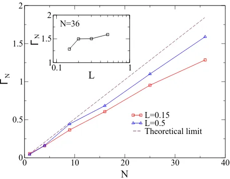
FIG. 7: (Color online) The Ringelmann effect in an array of sensors. The Signal-to-noise ratio ΓN as a function of the

numberN of sensors in the array. The array is organized into the square lattices (see Fig. 6) with the inter-sensor intervals

L. The target field is the weak periodic signalx=asin(Ωt), wherea = 0.001, Ω = 2π×0.01. The noisesξi(t) are

inde-pendent OU stochastic processes. The theoretical dependence is shown with the dashed line. It was found with Eq. (23). It is easy to see that the obtained results are always below the theoretical capacity. This is a sign of the Ringelmann ef-fect in our coupled array. The inset shows a clear increase in the summed SNR response (for fixedN = 36) as the sensor separation in the array increases, corresponding to a lower coupling strength.

IV. RESULTS AND DISCUSSION

Fig. 7 shows that, in the case of a weak periodic signal, the performance of the sensory system is better when the inter-sensor intervals are longer (weak coupling). It is easy to see that the obtained results are always below the capacity defined as the theoretical dependence.

0 10 20 30 40 0

50 100 150 200 250

L=1.0 L=0.25 L=0.2 L=0.18 Theoretical limit

0.1 1

0 50 100

N

Γ L

ΓN N=36

N

FIG. 8: (Color online) The Ringelmann effect in an array of sensors. Same parameters as Fig 7 but witha= 0.01

.

so that the SNR is reduced. It is easy to see that

Γactual<Γexpected≡

N

X

i=1

Γi,alone, i= 1..N. (24)

Comparing Eq. (1) and Eq. (24), we conclude that the inequality Eq. (24) satisfies the definition of the RE, with the one caveat: instead of the maximal productivity, we use the SNR in the system as a performance measure. The SNR is almost the same whether the sensor is opti-mally tuned or not, as long as the inputxof the transfer functionf(x, q) is within the dynamic range. Hence, the maximum SNR is equivalent to the optimal SNR. There-fore, we may use the term “Ringelmann Effect” in the context of the reduction of the SNR in the array of sen-sors.

In contrast to Fig. 7, Fig.8 shows that the SNR is a non-monotonic function of the number of the units in the array. In fact, there arises a situation wherein the number of mutual interactions grows faster than the number of units in the array. Every interaction makes its individual contribution to the positive feedback of the system and increases strength of the interactions.

Fig.8 (inset) shows that the reduction of the inter-sensor intervals L (meaning an increase in the coupling strength) leads to a reduction of the performance of the sensory system, i.e. the SNR rapidly drops. Obviously, there is a critical L that corresponds to a transition of the system behavior from the amplification of the exter-nal magnetic fields to the generation of a spontaneous magnetic field magnetization) that is mostly indepen-dent of external fields. This phenomena is similar to a phase transition [15]. An analogous effect is apparent as a function of N (see figure 8). For strong coupling (small separationL), the “self” fields (arising from the spontaneous magnetization of the core)of each sensor are amplified far more than the external magnetic field. In

0 10 20 30 40

0 0.5 1 1.5 2

Expected linear dependence Actual dependence Mitigated RE

N

A

FIG. 9: (Color online) The synergetic effect of the coupling on the gain in the array. HereA is the output amplitude of the array. The periodic input signal isx=acos Ωt. Param-eters: Ω = 2π×0.01,a= 0.01,δ = 0.01,T =τ = 10, and

L= 0.18. The expected theoretical dependence was obtained with Eq.(8) and assumption that the amplitude isA=N×A0,

whereA0is the amplitude of the unit (of the array)

perform-ing alone.

the largeL (i.e. weak coupling) limit the response ap-proaches the theoretical maximum, particularly for weak target signals. These two regimes are, loosely, connected via a maximum in the SN R vs. N curve as visible in figure 8. AsN decreases, the maximum shifts to a lower

N value.

To illustrate the influence of the coupling on the sen-sory system we consider a square matrix consisting of sensor elements that have the individual SNRs,

Γm,n=

c2

m,n

1−c2

m,n

, (25)

where the coefficientscm,nare

cm,n=

zm,ns−zm,ns

σzm,nσs ,

zm,n = f(s +ξm,n, qm,n), m = 1,· · ·,

√

N and n = 1,· · ·,√N.

We now consider the (numerical) results for the almost independent sensors, i.e. the sensors are weakly coupled due to the long inter-sensor intervals (we takeL= 1 for this case). It is easy to see that the individual signal-to-noise ratios Γm,nin all matrices are almost identical and

close to value of the SNR of the single sensor (N = 1). We illustrate this by using a strong signal (amplitudea= 0.01) and computing, for a single sensor, Γ1= 6.326391. For a 2D square lattice of varying size, we can calculate the individual signal-to-noise ratios Γm,nas:

N = 4:

6.159971 6.433196 6.456477 6.349792

Total Γ4is 22.818512.

N = 9:





6.297275 6.458169 6.403746 6.374942 6.431465 6.333464 6.556485 6.643418 6.327900



 (27)

Total Γ9 is 45.484923, and so on. It is easy to see that the total SNR is less than the sum of all SNRs, i.e. much redundant information passes through the sensory sys-tem.

Another illustrative example can be considered, wherein the coupling is strong due to the short inter-sensor intervals, L= 0.18. As in the preceding case we can calculate Γ1= 6.234534 for a single element. In this case, we find, as above,

N = 4:

11.158677 11.292682 11.451936 11.118461

(28)

Total Γ4is 23.293699.

N = 9:





14.360633 16.886906 14.651738 16.707638 19.346849 17.575212 14.750152 16.593489 15.213220



 (29)

Total Γ9is 33.708725.

The sensors are “cooperating”. The individual SNRs are greater than the SNR of the single sensor, and correla-tions between the individual responses of the sensors and the external signal are increased. But, the cooperative work counters the performance of the whole system; the total SNR is (for increasingN) below that of the weakly coupled sensors (the previous case for L= 1), with cor-relations between individual responses being increased in this case.

V. THE RINGELMANN EFFECT: SOCIOLOGY

MEETS PHYSICS

The coupling-induced phenomena detailed above bear resemblances to the phenomena described by Max Ringelmann 103 years ago [13]; the so-called Ringelmann Effect (RE) is frequently cited in the social sciences lit-erature [16, 17]. We believe the similarity is much more than a qualitative coincidence and is based on similar dynamical principles mediated by the coupling.

In his studies, Ringelmann focused on the maximum performance of humans involved in experiments wherein they used different methods to push or pull a load hor-izontally [13]. The RE has already been introduced in section I; here, we provide some more detail. Ringel-mann discriminated two main contributions to human productivity losses (see e.g. Fig. 10), namely the motiva-tion loss (now referred to in the contemporary literature as “social loafing”) and a ”coordination” loss; he concen-trated, however, on the coordination loss as an explana-tion for the reducexplana-tion of performance [17]. Ringelmann

0 1 2 3 4 5 6 7 8

0 100 200 300 400 500 600 700 800

Potential productivity Pseudogroups Actual groups

Motivation loss

Coordination loss

Obtained output

Size of group

Performance

FIG. 10: There are the two major causes of productivity losses in groups working on additive tasks. The portion between the dashed line and the dotted line represents motivation loss (social loafing), and the portion between the dotted line and the solid line represents coordination loss. “Pseudogroups” are defined as groups of individuals who were actually working alone, but thought they were working as part of a group. The design of the figure was adopted from Ref.[16].

believed that coordination loss was the more important contributor to the RE because similar reductions in per-formance occurred not only in groups of humans and ani-mals (horses and oxen [18]), but also in technical systems wherein social loafing was, clearly, impossible. For ex-ample, in multicylinder combustion engines, the engines with the larger number of cylinders produced less power per cylinder [13, 17].

One hundred years ago it was too difficult to cre-ate a mathematical description of the Ringelmann Effect (RE) because of a lack of understanding of complex sys-tems. Consequently, the co-ordination losses observed by Ringelmann have never been explained or understood. In contrast, the performance loss due to social loafing has been well studied by social scientists. They found that social loafing was not limited to groups that needed to exert physical effort. The social loafing could, in fact, be observed when groups worked at diverse tasks, e.g. maze performance [19], evaluating a poem [20], song writing [21], brainstorming [22], reacting to proposals [23], judg-mental tasks [24], research [25], software developing [26– 28], pumping air [29], clapping [30], rowing [31], pulling a rope [32], swimming in relay races [33], job selection decisions, typing, and creativity problems [16, 34].

In this work, we have studied (for a coupled sensor array) another type of contribution to productivity loss; this contribution stems from interactions between mem-bers of a group which we believe is also the origin of the co-ordination loss reported by Ringelmann. To illus-trate the interaction-induced loss we start by discussing the Ringelmann’s original experiments relating to a hu-man horizontally pulling a rope attached to a dynamome-ter [13]. In the experiments, the subject’s feet are in contact with the ground and the body slopes to create tension in the rope with the help of gravity; as the slope and hence pulling force increases so does the balancing frictional force on the ground. For some critical slope the pulling force equals the maximum sustainable fric-tional force giving rise to a “critical point”. Exceeding this slope (force) results in loss of stability. Thus, for the “best” performance, the subject should remain close to the critical point while not going past it (i.e.remain within the ’working range’). We can assume that the subject uses the following control “algorithm” to adjust (tune) his body to the critical position. The subject in-creases his slope until slippage starts to occur; he, then, stumbles backwards to correct the sliding. This process is then repeated with the subject trying to ’bias’ his po-sition as close to the critical point as possible without slipping. Near the critical point fluctuations are ampli-fied; therefore, the body of the subject moves randomly with multiple corrections required to prevent, or as a con-sequence of, slippage. If a group of humans are pulling the rope, unintentional random movement of one member will dramatically affect the “tuning” processes of other members of the group. To avoid loss of stability in the presence of common fluctuations, the members of the group will keep the positions of their bodies away from the critical state. Hence, the net performance of the hu-mans will be reduced.

In his pulling-the-rope experiments, Ringelmann asked the subjects to maintain a maximum effort for 4-5 s [13]. Given this relatively long duration it is not really con-ceivable that subjects were unable to pull at the same time i.e. they would have been able to synchronise their efforts. Consequently, the co-ordination losses measured by Ringelmann were, almost certainly, caused by the (un-intentional) movement of the rope that was fed-back to members through the mechanical coupling of the rope itself.

In this paper we have studied a physical system that is not similar to the group of humans in Ringelmann’s ex-periments, but the coupling-induced dynamics does have a similar impact on performance; the coupling channels fluctuations from individual sensor outputs to adjacent sensors which are themselves already optimally tuned (i.e. their dynamic range, and hence SNR, is maximised). The fluctuations therefore perturb the sensors away from their optimal working point thus lowering overall perfor-mance.

From an application perspective mitigation of the RE is necessary to enhance performance. We now provide a

possible path to mitigating the losses in arrays of nonlin-ear engineered devices.

Can the Ringelmann Effect be Mitigated?

According to Figs.(7) and (8), the RE can be mitigated by increasing the element separation L in the sensory array. But, in this case the size of the array will either become prohibitively large or result in sensors picking up different spatially localised signals. Hence an alternative way of reducing the RE is required.

Since the RE takes place due to the coupling between the sensory units we could, at least on paper, cancel the coupling termφiin Eq.(13) to improve the SNR response

of the array. However, in contrast to the mathematical model, the simple “cancellation of the coupling term” is usually impossible in a real sensory system. Therefore we construct the cancelling term Φc,i to the coupling term

φi in Eq. (13), from data available from measurements

in a possible real experiment; ideally, the cancelling term should be Φc,i = −φi. In keeping with our desire to

achieve the mitigation of the RE through realistic (i.e. experimentally accessible) scenarios, however, we assume that it is impossible to measure the quantityφi.

Accord-ing to Eq. (17), however, this quantity can be estimated from a knowledge of the parameters g, li,j, qi and zi,

where i = 1, ..., N. For simplicity, we will assume that the dynamics of all parametersqi are similar and all qi

take on almost the same values,qi ≃qj. Then the

can-celling term will be,

Φc,i=−g√qi N

X

j=1,i6=j

zj

li,j

, (30)

wherezj is the output of the jth unit. Hence, Eq. (13)

can be rewritten as,

zi=f(s+ξi(t) +φi+ Φc,i, qi). (31)

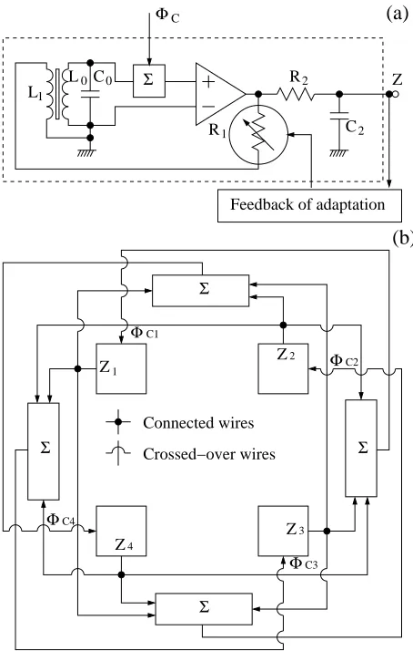
The term Φc,i in Eq. (31) implies a global feedback in

the sensory system, as shown in Fig. 11. In Fig. 11(a) the circuit of a single unit of the array with the output

z and the additive input Φc is shown. Fig. 11(b) shows

the global feedback for each unit. The results stemming from the feedbacks can be seen in Fig. 12. The SNR is significantly improved but the theoretical limit is not reached due to the (still) non-ideal structure of the can-celling term Φc,i(see Eq. (30)).

L Σ

R Z

C

Feedback of adaptation

(a)

(b)

Φ

R1 2

2 0C0

L

Σ

Φ

2

Z

C2

Crossed−over wires Connected wires

C

Z4

Z3

ΦC3

Σ

Z1 C1

Φ

Σ

ΦC4

Σ

FIG. 11: (a) The circuit of the sensory unit. Since the pa-rameterq should depend onR1, in the figure we show that

the variable resistor R1 is a target for the feedback of the

adaptation (self-tuning mechanism). (b) The complete sys-tem with 4 units. The blocks marked withP

are summators with different weights as required by Eq.(30).

system not only receives signals from inner hair cells but tries to control parameters of outer hair cells. Wecould speculate that the feedback circuits, OHCs → IHCs →

afferents → CNS → efferents →OHCs, schematized in figure 13 could play the role of a RE mitigating system. This is an interesting conjecture but nothing more than a conjecture at this point.

VI. CONCLUSIONS

In this work, we have introduced a model of an array of nonlinear interacting sensors. The individual sensors can be tuned to their optimal regimes for the best perfor-mance, when uncoupled. However, in the presence of the other sensors, this optimization (in the individual units) is lost because of coupling induced interaction. This is a “coupling” loss that can lead to a reduction in

perfor-0 10 20 30 40

0 50 100 150 200 250

Without a global feedback With the global feedback Theoretical limit

N ΓN

FIG. 12: (Color online) Mitigating the Ringelmann Effect in an array of sensors. Same parameters as Fig 8 with separation

L= 0.18.

mance of the entire sensory system.

The performance loss is most evident at smaller inter-sensor intervals (corresponding to higher coupling strength). The overall performance, quantified by a to-tal SNR, is bounded from above by the theoretical (or ideal) limit given by N ×ΓN=1 (Eq. (23)); this value is approached only in the limit wherein the sensors are, effectively, de-coupled.

Clearly, it would be a significant improvement if we could mitigate (or reduce) the losses stemming from the RE in a sensory array of the type considered in this work. One possible route to this, via global feedback, has been proposed. Eq. (30) derived from the feedbacks depends on both the geometrical parameters of the array (the sep-aration between sensorsli,j) and the outputs zi of the

individual units of the array. Note that Eq. (30) is an approximation of the ideal canceling term Φc,i = −φi

but, in contrast to the ideal cancellation term, it can be realized via the electrical circuit shown in Fig. 11. Since Φc,i differs from−φi (as already mentioned above), it is

not able to completely cancel the parasitic coupling φi

between the individual elements/sensors. Therefore, the theoretical limit of ideal performance cannot be reached in practice (unless the coupling is, identically, zero) and the RE still limits the array performance, albeit in a greatly reduced form.

(b)

OHC OHC

OHC IHC OHC

OHC OHC

IHC

CNS

Signal

Basilar Membrane − Tectorial

Membrane System

Efferents Afferents Mechanical coupling

Adaptation in the OHC

Tectorial Membrane

Basilar Membrane

System motor sensor

(a)

Signal

OHC

CNS

FIG. 13: (Color online) (a) The outer hair cell (OHC) in-teracting with the basilar membrane - tectorial membrane system and with the central nervous system (CNS) [35]. The OHC can schematically be split into the sensor and motor components. The dotted green loop shows that the sensory part of the OHC is adaptive subsystem [36]. (b) The coupling in the auditory system of mammals [37]. The afferents are shown with dash-dotted red arrows targeted to the CNS, and the efferents are shown with dashed blue arrows. Mechanical coupling between the OHCs, and inner hair cells (IHCs) and the basilar membrane - tectorial membrane system are shown with solid black arrows.

overall SNR performance and scaling it by N to yield the individual performances. Hence, unlike the results of the preceding section, all the component elements in each coupled array would have the same SNR response. For example, in theL= 0.18 case, we would obtain: Γ = 6.23 (N = 1), 5.82 (N = 4), 3.74 (N = 9), etc. Clearly, if the social scientists could, separately, quantify the individual performances of elements in their systems, their results might be similar to the results of this article.

At this point it is worth noting that there does in fact exist at least one exception (that we are aware of) in the social sciences literature, wherein the loafing and coor-dination losses were, separately, quantified. Latane et. al. [38] carried out an experiment involving clapping and shouting by a group of human subjects. Among the tests, one in particular stands out: participants were asked to shout as loudly as they could when alone, in pairs, in sixes, etc. The subjects were blindfolded and wearing headphones subject to a masking signal; therefore they

were unaware of the presence of other subjects. The tri-als included situations wherein the subjects (still blind-folded and wearing headphones) were led to believe that they were actually part of a group. A novel testing and measurement procedure allowed the researchers to quan-tify individual performances when the subjects knew they were alone, and when they thought they were in a group. This allowed the researchers to, separately, quantify the loafing and coordination losses in the group performance. The following extract, directly from the abstract of [38] is self-explanatory: “Two experiments found that when asked to perform the physically exerting tasks of clap-ping and shouting, people exhibit a sizable decrease in individual effort when performing in groups as compared to when they perform alone. This decrease, which we call social loafing, is in addition to losses due to faulty coordination of group efforts.”

Other problems in the quantification of human per-formance could arise when one confronts a heavy-tailed distribution of contributions of individual group mem-bers. For example, in an analysis of open source soft-ware production, it was reported that the distribution of contributions per software developer was heavy-tailed, meaning the first two statistical moments (mean and vari-ance) were undefined [28]. Due to the difficulty in cor-rectly defining the performance of software developers and due to problems relating to an estimation of this quantity from available data, the authors of two sepa-rate papers [26, 27] came to opposite conclusions regard-ing the presence of a Rregard-ingelmann effect in the software production process. It is easy to understand that a sim-ilar situation could arise in a sensory array when the TH sensors, that are the backbone of this paper, are replaced with different sensors that might be tuned to different critical behavior e.g. a phase transition [15] or self-organized criticality [39], instead of the Hopf bifurca-tion. Such sensors could be very sensitive to weak signals but their noise-floor distributions could be heavy-tailed. Clearly, then, if the first and second moments of the noise distributions are not defined then it will be difficult to correctly quantify the signal-to-noise ratio and estimate the performance of the sensory system.

but become less effective when coupled into a complex interacting network. We have demonstrated that, in ad-dition to the local optimization (adaptation), some form of global optimization, e.g via feedback, can help to mit-igate Ringelmann type effects. These principles are ex-pected to be generic across a wide class of nonlinear dy-namic systems.

It seems fitting to conclude this paper with an excla-mation point. While the coupling-induced loss and the RE can occur in many coupled nonliner dynamic sys-tems (see previous paragraph), it is the self-tuning to an optimal point (effectively poised on the threshold of the Andronov-Hopf bifurcation in our case) that is a

cen-tral feature of signal processing in the cochlea. Thus our sensor array (and, in fact, the single TH sensor as well) is not biomimetic unless we incorporate the self-tuning mechanism in each sensor prior to setting up the array.

Acknowledgments

ARB gratefully acknowledges funding by the Office of Naval Research Code 30; NGS and APN gratefully ac-knowledge funding by ONRG award N62909-11-1-7063, and useful discussions with R. P. Morse.

[1] W. Bialek, Ann. Rev. Biophys. Biophys. Chem.16, 455 (1987).

[2] K.-E. Kaissling, Ann. Rev. Neurosci.9, 121 (1986). [3] T. H. Bullock and F. P. J. Diecke, Journal of Physiology

134, 47 (1956).

[4] M. N. Coleman and D. M. Boyer, The Anatomcal Record 295, 615631 (2012).

[5] C. K˝oppl, O. Gleich, and G. A. Manley, Journal of Com-parative PhysiologyA 171, 695 (1993).

[6] G. A. Manley and J. A. Clack, inEvolution of the Ver-tebrate Auditory System, edited by G. A. Manley, A. N. Popper, and R. R. Fay (Springer - Verlag, New-York, 2004).

[7] G. A. Manley, PNAS97, 11736 (2000).

[8] P. Dobbins, Bioinspiration and Biomimetics2, 19 (2007). [9] J. Stroble, R. Stone, and S. Watkins, Sensor Review29,

112 (2009).

[10] A. P. Nikitin, N. G. Stocks, and A. R. Bulsara, Physical Review Letters109, 238103 (2012).

[11] S. Takeuchi and K. Harada, IEEE Trans. Magn. MAG-20, 1723 (1984).

[12] S. Camalet, T. Duke, F. Julicher, and J. Prost, PNAS 97, 3183 (2000).

[13] M. Ringelmann, Annales de l’Institut National Agronomique, 2e serieXII, 1 (1913).

[14] R. D. Driver, D. W. Sasser, and M. L. Slater, The Math-ematical Association Monthly80, 990 (1973).

[15] H. E. Stanley, Introduction to Phase Transitions and Critical Phenomena (Oxford University Press, Oxford and New York, 1971).

[16] D. R. Forsyth,Group Dynamics(Thomson/Wadsworth, Belmont, Calif., 2006), 4th ed.

[17] D. A. Kravitz and B. Martin, Journal of Personality and Social Psychology50, 936 (1986).

[18] M. Ringelmann, Annales de l’Institut National Agronomique, 2e serieVI, 243 (1907).

[19] J. M. Jackson and K. D. Williams, Journal of Personality and Social Psychology49, 937 (1985).

[20] R. E. Petty, S. G. Harkins, , K. D. Williams, and B. La-tane, Personality and Social Psychology Bulletin3, 579 (1977).

[21] J. M. Jackson and V. R. Padgett, Personality and Social Psychology Bulletin8, 672 (1982).

[22] S. G. Harkins and R. E. Petty, Journal of Personality and Social Psychology43, 1214 (1982).

[23] M. A. Brickner, S. G. Harkins, and T. M. Ostrom, Jour-nal of PersoJour-nality and Social Psychology51, 763 (1986). [24] W. Weldon and G. M. Gargano, Organizational Behavior

and Human Decision Processes36, 348 (1985).

[25] R. Kenna and B. Berche, Research Evaluation 20, 107 (2011).

[26] D. Sornette, T. Maillart, and G. Ghezzi, PLOS ONE9 (8), e103023 (2014).

[27] I. Scholtes, P. Mavrodiev, and F. Schweitzer, Empir. Soft-ware Eng.21, 642 (2016).

[28] T. Maillart and D. Sornette,

http://arxiv.org/abs/1608.03608 (2016).

[29] N. L. Kerr and S. E. Bruun, Personality and Social Psy-chology Bulletin7, 224 (1981).

[30] S. G. Harkins, B. Latane, and K. Williams, Journal of Experimental Social Psychology16, 457 (1980).

[31] C. J. Hardy and R. K. Crace, Journal of Sport and Ex-ercize Psychology13, 372 (1991).

[32] A. G. Ingham, G. Levinger, J. Graves, and Y. Peck-ham, Journal of Experimental Social Psychology10, 371 (1974).

[33] K. D. Williams, S. A. Nida, and B. Latane, Basic and Applied Social Psychology10, 73 (1989).

[34] J. A. Shepperd, Psychological Bulletin113, 67 (1993). [35] P. Dallos, The Journal of Neuroscience12, 4575 (1992). [36] R. Fettiplace and C. M. Hackney, Nature Reviews

Neu-roscience7, 19 (2006).

[37] H. Spoendlin, American Journal of Otolaryngology 6, 453 (1985).

[38] B. Latane, K. Williams, and S. Harkins, Journal of Per-sonality and Social Psychology37, 822 (1979).

[39] P. Bak, C. Tang, and K. Wiesenfeld, Physical Review Letters59, 381 (1987).

[40] J. M. Beckers, Annu. Rev. Astron. Astrophys. 31, 13 (1993).

[41] N. Hur and K. Nam, IEEE Transactions on Industrial Electronics47, 871 (2000).