Calibration with confidence : a principled method for panel assessment

warwick.ac.uk/lib-publications

Original citation:

MacKay, R. S. (Robert Sinclair), Kenna, R., Low, R. J. and Parker, S.. (2017) Calibration with

confidence : a principled method for panel assessment. Royal Society Open Science, 4 .

160760.

Permanent WRAP URL:

http://wrap.warwick.ac.uk/86321

Copyright and reuse:

The Warwick Research Archive Portal (WRAP) makes this work of researchers of the

University of Warwick available open access under the following conditions.

This article is made available under the Creative Commons Attribution 4.0 International

license (CC BY 4.0) and may be reused according to the conditions of the license. For more

details see:

http://creativecommons.org/licenses/by/4.0/

A note on versions:

The version presented in WRAP is the published version, or, version of record, and may be

cited as it appears here.

rsos.royalsocietypublishing.org

Research

Cite this article:MacKay RS, Kenna R, Low RJ, Parker S. 2017 Calibration with confidence: a principled method for panel assessment. R. Soc. open sci.4: 160760.

http://dx.doi.org/10.1098/rsos.160760

Received: 29 September 2016 Accepted: 9 January 2017

Subject Category:

Mathematics

Subject Areas:

applied mathematics

Keywords:

calibration, evaluation, assessment, confidence, uncertainty, model comparison

Author for correspondence:

R. Kenna

e-mail:[email protected]

In memory of Prof. Sir David John Cameron MacKay (22 April 1967–14 April 2016).

Calibration with confidence:

a principled method for

panel assessment

R. S. MacKay

1

, R. Kenna

2

, R. J. Low

2

and S. Parker

1

1_{Mathematics Institute and Centre for Complexity Science, University of Warwick,}

Coventry CV4 7AL, UK

2_{Applied Mathematics Research Centre, Coventry University, Coventry CV1 5FB, UK}

RK,0000-0001-9990-4277

Frequently, a set of objects has to be evaluated by a panel of assessors, but not every object is assessed by every assessor. A problem facing such panels is how to take into account different standards among panel members and varying levels of confidence in their scores. Here, a mathematically based algorithm is developed to calibrate the scores of such assessors, addressing both of these issues. The algorithm is based on the connectivity of the graph of assessors and objects evaluated, incorporating declared confidences as weights on its edges. If the graph is sufficiently well connected, relative standards can be inferred by comparing how assessors rate objects they assess in common, weighted by the levels of confidence of each assessment. By removing these biases, ‘true’ values are inferred for all the objects. Reliability estimates for the resulting values are obtained. The algorithm is tested in two case studies: one by computer simulation and another based on realistic evaluation data. The process is compared to the simple averaging procedure in widespread use, and to Fisher’s additive incomplete block analysis. It is anticipated that the algorithm will prove useful in a wide variety of situations such as evaluation of the quality of research submitted to national assessment exercises; appraisal of grant proposals submitted to funding panels; ranking of job applicants; and judgement of performances on degree courses wherein candidates can choose from lists of options.

1. Introduction

This paper addresses the widespread problem of how to take into account differences in standards, confidence and bias in assessment panels, such as those evaluating research quality or grant proposals, employment or promotion applications, and classification of university degree courses, in situations where it is not feasible for every assessor to evaluate every object to be assessed.

2

rsos

.ro

yalsociet

ypublishing

.or

g

R.

Soc

.open

sc

i.

4

:1

60760

...

Table 1.Panel Assessment Methods. The matrix of four approaches according to use of calibration and/or confidences. Simple averaging (SA) is the base for comparisons. Fisher’s IBA does not deal with varying degrees of confidence and the confidence-weighted averaging does not achieve calibration. The method proposed herein (CWC) accommodates both calibration and confidences.

without confidences with confidences

without calibration simple averaging (SA) confidence-weighted averaging (CWA)

. . . .

with calibration incomplete block analysis (IBA) calibration with confidence (CWC)

. . . .

A common approach to assessment of a range of objects by such a panel is to assign to each object the average of the scores awarded by the assessors who evaluate that object. This approach is represented by the cell labelled ‘simple averaging’ (SA) in the top left of a matrix of approaches listed intable 1, but it ignores the likely possibility that different assessors have different levels of stringency, expertise and bias [1]. Some panels shift the scores for each assessor to make the average of each take a normalized value, but this ignores the possibility that the set of objects assigned to one assessor may be of a genuinely different standard from that assigned to another. For an experimental scientist, the issue is obvious:calibration.

One solution is to seek to calibrate the assessors beforehand on a common subset of objects, perhaps disjoint from the set to be evaluated [2]. This means that they each evaluate all the objects in the subset and then some rescaling is agreed to bring the assessors into line as far as possible. This would not work well, however, in a situation where the range of objects is broader than the expertise of a single assessor. Also, regardless of how well the assessors are trained, differences between individuals’ assessments of objects remain in such ad hoc approaches [3].

If the expertise of two assessors overlap on some subject, however, any discrepancy between their evaluations can be used to infer information about their relative standards. Thus, if the graphΓA on the set of assessors, formed by linking two whenever they assess a common object, is sufficiently well connected, one can expect to be able to infer a robust calibration of the assessors and hence robust scores for the objects. The construction of this graph is illustrated infigure 1, beginning from the graph Γ showing which objects are assessed by which assessors.

One approach to achieving such calibration was developed by Fisher [4], in the context of trials of crop treatments. Denoting the score from assessorafor objectobysao, Fisher’s approach is based on fitting

a model of the formsao=vo+ba+εaowithεaoindependent identically distributed random variables of

mean zero. Thenbais the bias inferred for assessoraandvois the value inferred for objecto. Fisher’s

approach is known asadditive incomplete block analysis(IBA) and a body of associated literature and applications has since been developed (e.g. [5]), though its use in panel assessment seems rare. It is represented as the bottom left entry oftable 1.

Another ingredient that is important in many panel assessments, however, is different weights that may be put on different assessments. We refer to these weights as ‘confidences’. Fisher’s IBA does not take different levels of confidence into account.

If the assessors express confidences in the assessments, for example, by some pre-determined weights assigned to types of assessment or by the assessors declaring confidences in each of their scores, then it is natural to replace SA by confidence-weighted averaging. This is represented as the top right entry of table 1, but it does not address the calibration issue so we do not consider it further.

In this paper, we present and test a method to calibrate scores taking into account confidences; that is, we complete the matrix of approaches represented intable 1, where our method is termedcalibration with confidence(CWC). We demonstrate that the method can achieve a greater degree of accuracy with fewer assessors than either SA or IBA, and we derive robustness estimates taking the confidences into account. We are aware of two other schemes that incorporate confidences into a calibration process. One is the abstract-review method for the SIGKDD’09 conference (section 4 of [6]; see also [7]). The other is the abstract-review method used for the NIPS2013 conference (building on [8] and described in [9]). Our method has the advantages of simplicity of implementation and a straightforward robustness analysis. We leave detailed comparison with methods such as these for future publication.

2. The model

3

rsos

.ro

yalsociet

ypublishing

.or

g

R.

Soc

.open

sc

i.

4

:1

60760

...

a₁

a₂

a₃

a₄

o₁

o₂

o₃

o₄

o₅

o₆

objects assessors

o₁

o₂

o₃

o₄

o₅

o₆

a₁

a₂

a₃

a₄

o₁

o₂

o₃

o₄

o₅

o₆

a₁

a₂

a₃

a₄

a₁ a₂

a₄ a₃

a₁ a₂

a₄ a₃

a₁ a₂

a₃ a₄

G GA

(a)

(b)

(c)

Figure 1.Three examples of assessment graphsΓ showing which objectojis assessed by which assessorak, and the resulting graphs

ΓAon the set of assessors where two assessors are linked if they assess an object in common. Case (a) produces a fully connected assessor

graph, (b) a moderately connected graph, whereas case (c) is disconnected.

is a real number related to a ‘true’ valuevofor the object by

sao=vo+ba+εao, (2.1)

wherebacan be called thebiasof assessoraandεaoare independent zero-mean random variables. Such

a model forms the basis for additive IBA. This was also proposed in ref. [10] (see eqn (8.2b) therein) but without a method to estimate the true values. Here we will achieve this and make a significant improvement, namely the incorporation of varying confidences in the scores.

To take into account the varying expertise of the assessors with respect to the objects, we propose that in addition to the scoresao, each assessor is asked to specify a level of confidence for that evaluation. This

could be in the form of a rating such as ‘high’, ‘medium’, ‘low’, as requested by some funding agencies, but we propose to allow something more general and akin to experimental science. Confidence can be estimated by asking assessors to specify an uncertaintyσao>0 for their score and then the confidence

level (or ‘precision’) is taken to be

cao= 1 σ2 ao

. (2.2)

The instructions to the assessors can be to choosesaoandσaoso that23of their probability distribution for

the score lies in [sao−σao,sao+σao],16 above this interval and16 below it. Methods for training assessors

4

rsos

.ro

yalsociet

ypublishing

.or

g

R.

Soc

.open

sc

i.

4

:1

60760

...

So let us suppose that

εao=σaoηao, (2.3)

withηaoindependent zero-mean, random variables of common variancew. For the moment, we setw=1;

extensions to other values ofware considered in appendix A, and in particular are necessary if confidence is expressed only qualitatively. In the case that confidences are reported as only high, medium or low, they can be converted into quantitative ones by for example choosingλ≈2 and settingcao=λ2, 1,λ−2,

respectively. The interpretation ofλis the ratio of the uncertainty for a low confidence evaluation to that for a medium one, and for a medium one to a high one. Thenwis unspecified but can be fit from the data, as in appendix A.

Thus, our basic model is

sao=vo+ba+σaoηao. (2.4)

3. Solution of the model

Given the data{(sao,σao) : (a,o)∈E} for all assigned assessor–object pairs, we wish to extract the true

valuesvoand assessor biasesba. The simplest procedure is to minimize the sum of squares

(a,o)∈E η2

ao=

(a,o)∈E

cao(sao−vo−ba)2, (3.1)

where the confidence levelcaowas defined in equation (2.2). This procedure can be justified if theηaoare

assumed to be normally distributed, because then it gives the maximum-likelihood values forvoandba.

It can also be viewed as orthogonal projection of the vectorsof scoressaoto the subspace of the form

sao=vo+bain the Riemannian metric given by|s| =aocaos2ao.

Now expression (3.1) is minimized with respect tovoiff

a:(a,o)∈E

cao(sao−vo−ba)=0,

and with respect tobaiff

o:(a,o)∈E

cao(sao−vo−ba)=0.

It is notationally convenient to extend the sums to all assessors (respectively objects) by assigning the valuecao=0 to any assessor–object pair that is not inE(i.e. for which a score was not returned). Then

these conditions can be written as

Covo+

a

bacao=Vo (3.2)

and

o

caovo+Caba=Ba. (3.3)

Here,

Vo=

a

caosao (3.4)

is the confidence-weighted total score for objectoand

Ba=

o

caosao (3.5)

is that for assessora,

Co=

a

cao (3.6)

is the total confidence in the assessment of objectoand

C_a=

o

cao (3.7)

5

rsos

.ro

yalsociet

ypublishing

.or

g

R.

Soc

.open

sc

i.

4

:1

60760

...

Equations (3.2) and (3.3) form a linear system of equations for the vo and ba. It has an obvious

degeneracy in that one could add a constant kto all thevoand subtractkfrom all thebaand obtain

another solution. One can remove this degeneracy by, for example, imposing the condition

a

ba=0. (3.8)

This is the simplest possibility and corresponds to a translation (shift) that brings the average bias over assessors to zero. Alternatives are discussed in appendix B.

Define a graphΓ linking assessorato objectoif and only if (a,o)∈E, as illustrated in the left column offigure 1. The edges in the graph are weighted by the confidencescao. Whether the set of equations (3.2)

and (3.3) has a unique solution after breaking the degeneracy depends on the connectivity ofΓ. Define a linear operatorLby writing equations (3.2) and (3.3) as

L

v

b

=

V B

, (3.9)

wherev,b,VandBdenote the column vectors formed by thevo,ba,VoandBa, respectively. The operator

Lhas null space of dimension equal to the number of connected components of Γ (this follows from Perron–Frobenius theory, e.g. [13]). Thus, ifΓ is connected, the null space ofLhas dimension one, so corresponds precisely to the null vectorsvo=k∀o,ba= −k∀a, that we already noticed and dealt with.

Connectedness ofΓ ensures that if (3.9) has a solution then there is a unique one satisfying (3.8). It remains to check that the right-hand side of equation (3.9) lies in the range ofL, thus ensuring that a solution exists. This is true if all null forms of the adjoint operatorL†send the right-hand side to zero. The null space ofL†has the same dimension as that ofL, becauseLis square, and an obvious non-zero null formαis given by

α(v,b)=

o vo−

a

ba. (3.10)

It follows from the definitions ofVandBthatα(V,B)=0. So a solution exists.

Thus, under the assumption that the assessor–object graphΓ is connected, equations (3.2) and (3.3) have a unique solution (v,b) satisfying equation (3.8). Note that connectedness of Γ is necessary for uniqueness, otherwise one could follow an analogous procedure, adding and subtracting constants independently in each connected component ofΓ, and thereby produce more solutions.

Equations (3.2) and (3.3) have a special structure, due to the bipartite nature ofΓ, that can be worth exploiting. The first equation (3.2) can be written as

vo=Vo−

abacao

Co . (3.11)

This can be substituted into the second equation (3.3) to obtain

a

Caaba−C_aba=

o

caoVo

Co −Ba, (3.12)

where

Caa=

o

caoca_o

Co (3.13)

can be considered as weights on the edges of the graphΓAon assessors illustrated in the right column of

figure 1. The dimension of the reduced system (3.12) is the numberNAof assessors (rather than the sum

of the numbers of assessors and objects), which gives some computational savings. Replacing one of the equations in (3.12), say that for the ‘last’ assessor, by equation (3.8) gives a system with a unique solution that can be solved forbby any method of numerical linear algebra, e.g. LUP decomposition [14]. Thenv can be obtained from equation (3.11).

A slightly more sophisticated approach to incorporating a degeneracy-breaking condition into equations (3.12) is described in appendix B.

6

rsos

.ro

yalsociet

ypublishing

.or

g

R.

Soc

.open

sc

i.

4

:1

60760

...

4. Case studies

We have tested the approach in three contexts. We report in detail on two case studies here. In the first case study, we use a computer-generated set of data containing true values of assessed items, assessor biases and confidences for the assessments and resulting scores. This has the advantage of allowing us to compare the values obtained by the new approach with the true underlying value of each item. The second case study is an evaluation of grant proposals using realistic data based on a university’s internal competition. In this test, of course, there is no possibility to access ‘true’ values, so instead we compare the evidence for the models using a Bayesian approach (appendix E), and we compare their posterior uncertainties (appendix D). The third context in which we tested our method was assessment of students; we report briefly on this at the end of the section.

4.1. Case study 1: simulation

In the simulation,NO=3000 objects are assessed by a panel of NA=15 assessors. This choice was

motivated by the number of outputs and reviewers in the applied mathematics unit of assessment at the UK’s 2008 research assessment exercise. The simulation was carried out using Matlab, and the system of equations was solved using its built-in procedure, which computed the LU decomposition ofL(with the last row replaced by the degeneracy-breaking condition (3.8)). The reduction to (3.12) was not used becauseNO=3000 is easily handled by modern personal computers.

True values of the itemsvowere assumed to be normally distributed with a mean of 50 and standard

deviation set to 15, but withvovalues truncated at 0 and 100. The assessor biasesbawere assumed to be

normally distributed with a mean of 0 and a standard deviation of 15. Each assessment was considered to be done with high, medium or low confidence, and these were modelled using scaled uncertainties for the awarded scores, ofσao=5, 10 or 15, respectively. The allocated scores follow equation (2.4), but

truncated at 0 and 100.

Withrassessors per item (which we took to be the same for each item in this instance), each simulation generated rNO object scores sao. From these, we generated NO value estimatesvˆo andNA estimates

of assessor biasesbˆausing the calibration processes. We then took the mean and maximum values of

the errors in the estimates,dvo= |ˆvo−vo|anddba= |ˆba−ba|. Simple averaging also delivered a value

estimatevˆo, as well as mean and maximal values of the errorsdvo. Finally, we determined the averages

of the errorsdvoanddbaover 100 simulations. The results for these averaged mean and maximal errors

in the scores are denoted bydvand (dv)max, respectively, and those for the biases (for the calibrated

approaches only) are denoteddband (db)max.

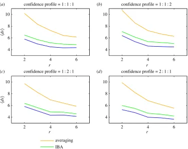
Results for all three methods are presented in figures2–4. The mean and maximal errors for the SA approach, the IBA method and the CWC approach are given in figures2a–dand3a–d. For demonstration purposes, we use three confidence levels rather than a continuous distribution. This allows us to clearly control differences in confidence levels in figures2and3and we do so by presenting four panels labelled (a)–(d). These represent different profiles, with the confidence for each assessment randomly allocated using probabilities for high, medium and low confidences in the ratios: (a) 1 : 1 : 1, (b) 1 : 1 : 2, (c) 1 : 2 : 1 and (d) 2 : 1 : 1. We observe that, for each method, the scores become more accurate (errors decrease) as the number of assessors per objectrincreases.

Fromfigure 2a–d, with only two assessors per object, the SA method gives errors averaging about 10 points. Overr=6 assessors per object are required to bring the mean error down to six points. Fisher’s IBA, however, achieves this level of improvement with only two or three assessors. The CWC method delivers a further level of improvement of about one point. One also notes that, for the calibration approaches, relatively little is gained on average by employing more than four assessors per object. This result can be compared with [15] which found that five assessors per object was optimal in terms of accuracy over cost, for a procedure used by the Canadian Institutes of Health Research.

Figure 3shows that IBA also leads to significant improvements in the maximal error values relative to those obtained through SA. With two assessors per object, maximal errors are reduced from about 45 to 30–35. The CWC approach does not appear to significantly improve upon this. However, with six assessors per object the maximal error value of about 25 delivered by the SA process is reduced to about 20 by IBA and to as low as 16 by CWC when half the assessments are done with a high degree of confidence in the scores.

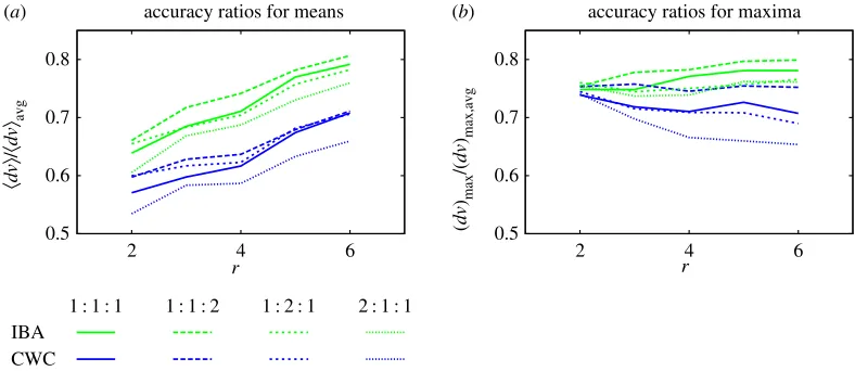
Figure 4a gives the improvements achieved by the calibration methods as ratios of the mean errors coming from Fisher’s IBA approach to the SA approachdvIBA/dvavgand of the mean errors

7

rsos

.ro

yalsociet

ypublishing

.or

g

R.

Soc

.open

sc

i.

4

:1

60760

...

4 6 8 10

2 4 6

·

dv

Ò

confidence profile = 1 : 1 : 1

4 6 8 10

2 4 6

confidence profile = 1 : 1 : 2

4 6 8 10

2 4 6

·

dv

Ò

r

confidence profile = 1 : 2 : 1

4 6 8 10

2 4 6

r

r r

confidence profile = 2 : 1 : 1

averaging IBA CWC

(a) (b)

(c) (d)

Figure 2.Mean errors plotted against the numberrof assessors per object for the SA approach (upper curves, orange), the incomplete-block-analysis method (middle curves, green) and the calibration-with-confidence approach (lower curves, blue). The various panels represent different confidence profiles with probabilities for high, medium and low confidences in the ratios: (a) 1 : 1 : 1, (b) 1 : 1 : 2, (c) 1 : 2 : 1 and (d) 2 : 1 : 1.

accuracy on the part of the calibrated approaches.Figure 4bgives the analogous accuracy ratios for the maximal errors, namely (dv)max,IBA/(dv)max,avgand (dv)max,CWC/(dv)max,avg.Figure 4ademonstrates

that IBA delivers mean errors between about 60 and 80% of those coming from the SA approach, the better improvements being associated with lower assessor numbers. This is also the most desirable configuration for realistic assessments, as it represents employment of a minimal number of assessors per object. The CWC approach reduces errors by about a further 10 percentage points irrespective of the number of assessors.

4.2. Case study 2: grant proposals

To test CWC in a realistic setting, we adapted data from a university’s internal competition for research funding, in which 43 proposals were evaluated by a panel of 11 assessors. Each proposal was graded by two assessors, who in addition each specified a confidence level in their grading in the form of high, medium or low. To respect confidentiality of the competition while making the data available, we not only anonymized the proposals and assessors but also made sufficient changes to the data (while preserving the statistical properties) so that attribution would not be possible. The actual panel used SA, but the assessors were also asked to provide confidences so that CWC could be applied for comparison. The panel awarded grants to the top 10 proposals. Our goals were firstly to see what differences would have been made by use of IBA or CWC, secondly to quantify the evidence for the three models from the data to determine which was most appropriate, and thirdly to compare the posterior uncertainties they provide.

To apply CWC, we translated the qualitative confidence levels of high, medium and low to values

cao=λ2, 1,λ−2, respectively, withλ=1.75. We choseλ=1.75 as a reasonable guess at how the assessors

8

rsos

.ro

yalsociet

ypublishing

.or

g

R.

Soc

.open

sc

i.

4

:1

60760

...

10 20 30 40 50

2 4 6

(

dv

)max

confidence profile =1 : 1 : 1

10 20 30 40 50

2 4 6

confidence profile = 1 : 1 : 2

10 20 30 40 50

2 4 6

(

dv

)max

r

confidence profile = 1 : 2 : 1

10 20 30 40 50

2 4 6

r

r r

confidence profile = 2 : 1 : 1

averaging IBA CWC

(a) (b)

(c) (d)

Figure 3.Maximum errors plotted against the numberrof assessors per object for the SA approach (upper curves, orange), the incomplete-block-analysis method (middle curves, green) and the calibration-with-confidence approach (lower curves, blue). The various panels represent different confidence profiles with probabilities for high, medium and low confidences in the ratios: (a) 1 : 1 : 1, (b) 1 : 1 : 2, (c) 1 : 2 : 1 and (d) 2 : 1 : 1.

0.5 0.6 0.7 0.8

2 4 6

·

dv

Ò

/

·

dv

Òavg

r

accuracy ratios for means

0.5 0.6 0.7 0.8

2 4 6

(

dv

)max

/(

dv

)max,avg

r

accuracy ratios for maxima

IBA

1 : 1 : 1 1 : 1 : 2 1 : 2 : 1 2 : 1 : 1

CWC

(a) (b)

Figure 4.(a) The ratiosdvIBA/dvavganddvCWC/dvavgmeasure the mean improved accuracies of IBA (green curves) and CWC

(blue), respectively, over SA. Smaller ratios indicate a greater degree of improvement over SA. (b) The analogous quantities for maximal errors are (dv)max,IBA/(dv)max,avgand (dv)max,CWC/(dv)max,avg, respectively. The four line types correspond to relative probabilities of

standard deviations of 5, 10 or 15, respectively, in the ratios 1 : 1 : 1 (solid); 1 : 1 : 2 (long-dashed); 1 : 2 : 1 (short-dashed) and 2 : 1 : 1 (dotted lines).

is for panel chairs to ask assessors to provide uncertainties rather than qualitative confidence levels, as indicated in §2, so we did not implement the inference ofλ.

9

rsos

.ro

yalsociet

ypublishing

.or

g

R.

Soc

.open

sc

i.

4

:1

60760

...

0 20 40 60 80 100

20 40 60 80 100

IB

A

SA

0 20 40 60 80 100

20 40 60 80 100

CWC

IBA

0 20 40 60 80 100

20 40 60 80 100

SA

CWC

–30 –20 –10 0 10 20 30

30 40 50 60 70 80 90

dif

ferences

means

(a) (b)

(c) (d)

Figure 5.Correlations between the results coming from the three methods applied to Case Study 2. The three panels give the correlations between the outputs of (a) IBA and SA; (b) CWC and IBA and (c) SA and CWC. The coefficients of determination are given, respectively, byR2=0.5701; 0.8807 and 0.3772. Panel (d) is a Bland–Altman or Tukey mean-difference plot of differences between results from pairs of approaches against their averages. The symbols ‘+’ (red) compare CWC to IBA (VCWC−VIBAversus (VIBA+VCWC)/2); ‘×’ (green)

compare IBA to SA (VIBA−Vavgversus (Vavg+VIBA)/2); ‘◦’ (blue) compare SA to CWC (Vavg−VCWCversus (VCWC+Vavg)/2).

Table 2.The 43 grant proposals are identified as OA, OB, OC,. . .OZ, OA, OB,. . .OP, OQ. Here they are ranked according to theirVavg,

VIBAandVCWCvalues, representing the outcomes of SA, the IBA and CWC approaches. Proposals identified by CWC as belonging to the

top 10 but missed by IBA are highlighted in boldface. Proposals identified by IBA or CWC as belonging to the top ten but missed by SA are highlighted in italics. Proposals which are not in the CWC top 10 are underlined.

rank SAVavg IBAVIBA CWCVCWC

1 OH (87.0) OA (85.3) OA (88.8)

. . . .

2 OP (87.0) OC (84.9) OB(85.2)

. . . .

3 OC (86.0) OH (80.6) OC (84.9)

. . . .

4 OS (84.0) OP (79.7) OD(82.8)

. . . .

5 OA (80.5) OD(79.5) OE(82.0)

. . . .

6 OM (80.5) OB(79.4) OF (78.9)

. . . .

7 OZ (80.5) OF (78.6) OG(78.4)

. . . .

8 OF (79.5) OE(76.9) OH (77.3)

. . . .

9 OA(78.5) OS (76.7) OI(77.1)

. . . .

10 OI (78.0) OJ(76.4) OJ(75.6)

. . . .

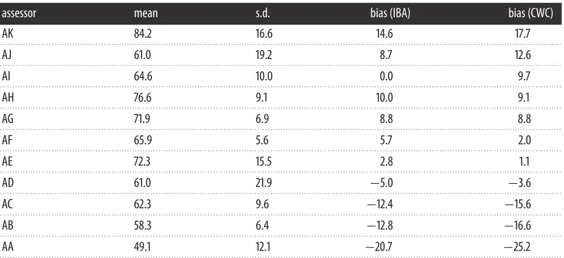
plot [16]. The correlations are not strong, though as we would expect, the correlation of IBA with CWC is stronger than those of either with SA. In particular, we note that the set of proposals rated in the top 10 varies substantially with the method used (table 2). The reason for the differences is that IBA and CWC attribute a significant range of biases to the assessors (table 3).

10

rsos

.ro

yalsociet

ypublishing

.or

g

R.

Soc

.open

sc

i.

4

:1

60760

...

Table 3.Assessor statistics: assessors are labelled AA,. . .AK according to increasing CWC-biases (5th column). Here, we give the mean scores they awarded, standard deviations and IBA-biases too. The mean score awarded over all assessments was 66.9.

assessor mean s.d. bias (IBA) bias (CWC)

AK 84.2 16.6 14.6 17.7

. . . .

AJ 61.0 19.2 8.7 12.6

. . . .

AI 64.6 10.0 0.0 9.7

. . . .

AH 76.6 9.1 10.0 9.1

. . . .

AG 71.9 6.9 8.8 8.8

. . . .

AF 65.9 5.6 5.7 2.0

. . . .

AE 72.3 15.5 2.8 1.1

. . . .

AD 61.0 21.9 −5.0 −3.6

. . . .

AC 62.3 9.6 −12.4 −15.6

. . . .

AB 58.3 6.4 −12.8 −16.6

. . . .

AA 49.1 12.1 −20.7 −25.2

. . . .

Table 4.Residuals (scaled by mean confidence in the case of CWC).

method SA IBA CWC

residual 8602 4388 3156

. . . .

Table 5.Bayesian log-evidences.

method SA IBA CWC

log-evidence −385 −389 −387

. . . .

A first answer is to compare the ‘residuals’ that the methods leave after the least-squares fit. In the case of SA, this means the value of equation (3.1) obtained by taking thevoto be the averaged scores and

ba=0. For IBA, the residual is the value of (3.1) at the least-squares fit, taking all thecao=1. For CWC,

we take the value of (3.1) at the least-squares fit, divided by the average confidence over all assessments. The residuals are presented intable 4. From this point of view, we see clear improvement progressively from SA to IBA to CWC, providing an apparently compelling argument for the use of CWC.

As IBA and CWC have more free parameters (the biases) than SA, however, one should penalize them appropriately to make a correct comparison. Also although normalizing the residual for CWC by the average confidence sounds sensible, it is not clear it is the right way to compare CWC with IBA.

A principled answer is provided by Bayesian model comparison. In this procedure, the evidence provided by the data in favour of each model is quantified, and the best model is the one with the highest evidence. The procedure to quantify the evidence for the three models is described in appendix E. It depends on assumptions about the prior probability distribution for the parameters of the models, but we took ‘ball’ priors on the true values and on the biases (constrained by the degeneracy-breaking condition) and a truncated Jeffreys’ prior on the variance of the noise. In the notation of appendix E, the parameters for the prior probability distributions were σO=22.5, σA=15,wmax=900, wmin=1.

As the evidences come out to be small numbers (around 10−168), we took their (natural) logarithms. The resulting log-evidences are shown intable 5. Simple averaging wins, but these values are so close together that we cannot make a strong conclusion about which method is most justified by the data. Furthermore, adjusting the prior probability distributions and the confidence weights changes which method has the highest evidence. We suspect that differences between the evidences for the models would become apparent if each proposal had been evaluated by more than two assessors.

11

rsos

.ro

yalsociet

ypublishing

.or

g

R.

Soc

.open

sc

i.

4

:1

60760

...

Table 6.Confidence-weighted root mean square uncertainties for the values (and biases in the cases of IBA and CWC). For SA, the weighting is according to the numbernoof assessors for objecto.

method SA IBA CWC

uncertainty 14.1 8.4 8.0

. . . .

one-third chance of differing by more than eight from the outputted values. This means that for IBA and CWC, only the top three proposals oftable 2are reasonably assured of being in the top 10.

As the object of the competition was only to choose the best 10 proposals to fund, rather than assign values to each proposal, it might have been more appropriate to design just a classifier system (with a tunable parameter to make the right number in the ‘fund’ class) but our goal was to use it as a test of CWC.

The fact that three different methods with roughly equal evidence lead to drastically different allocation of the grants, and with large posterior uncertainties, highlights that better design of the panel assessment was required. Large variability of outcome even when just using SA but with different assessment graphs was already noted by Graveset al. [17]. A moral of our analysis is that to achieve a reliable outcome, the assessment procedure needs substantial advance design. We continue a discussion of design in appendices C and F, but substantial treatment is deferred to a future paper.

4.3. Third context: assessment of students

We also tested the method on undergraduate examination results for a degree with a flexible options system [18] and on the assessment of a multi-lecturer postgraduate module.

In the former case, as surrogates for the confidences in the marks we took the number of Credit Accumulation and Transfer Scheme (CATS) points for the module, which indicate the amount of time a student is expected to devote to the module (for readers used to the European credit transfer and accumulation system, 2 CATS points are equivalent to 1 ECTS point). The amount of assessment for a module is proportional to the CATS points. If it can be regarded as consisting of independent assessments of subcomponents, e.g. one per CATS point, with roughly equal variances, then the variance of the total score would be proportional to the number of CATS points. As the score is then normalized by the CATS points, the variance becomes inversely proportional to the CATS points, making confidence directly proportional to CATS points. The outcome of our analysis indicated significant differences in standards for the assessment of different modules, but as most modules counted for 15 or 18 CATS, this was not a strong test of the merits of including confidences in the analysis, so we do not report on it here. For the postgraduate module, there were four lecturers plus module coordinator, who each assessed oral and written reports for some but not all of the students, according to availability and expertise (except the coordinator assessed them all). Each assessor provided a score and an uncertainty for each assessment. The results were combined using our method and the resulting value for each student was reported as the final mark. The lecturers agreed that the outcome was fair.

5. Discussion

We have presented and tested a method to calibrate assessors in a panel, taking account of differences in confidence that they express in their assessments. From a test on simulated data we found that calibration with confidence (CWC) generated closer estimates of the true values than Additive incomplete block analysis (IBA) or simple averaging (SA). A test on some real data, however, provided little evidence to distinguish between the methods, though they produced wildly different rankings, suggesting that the assessment procedure for that context needed more robust design. Nevertheless, CWC came ahead on posterior precision. We note that the default of assuming all assessment confidences to be equal results in IBA, which already represents a useful improvement over SA.

One of the principal conclusions from our analysis is that to achieve reliable outcomes from the methods we tested, requires good design of the assessment graph (showing which objects are evaluated by which assessors and with what confidences).

12

rsos

.ro

yalsociet

ypublishing

.or

g

R.

Soc

.open

sc

i.

4

:1

60760

...

Some other drawbacks of our CWC method are:

— It requires assessors to give reliable uncertainties; if assessors differ in their confidence estimates the method gives higher weight to those who give higher confidences. In particular, one needs to guard against an assessor giving unwarrantedly high confidence for a particular assessment. There is a case for calibrating confidences too.

— Bias effects may be more subtle than just an additive effect; for example, an assessor may be more generous (or perhaps tougher) on topics in which they have high confidence, or they may use a shorter or longer part of the scale than other assessors.

— Some organizations insist on round-number scores; this goes against the spirit of our approach and is awkward for assessors who may rightly wish to rate an object as between two of the allowed grades. The requirement is perhaps based on the laudable idea of not wishing to imply higher accuracy than is warranted, yet in our opinion this is better dealt with by reporting an uncertainty for each result on a continuous scale.

— Some organizations may insist that scores cannot go beyond certain limits, which is awkward for an assessor if after evaluating several objects highly they find there are some they wish to rate even higher.

There are a number of refinements which one could introduce to the core method, addressing some of these drawbacks. These include how to deal with different types of bias, different scales for confidence, different ways to remove the degeneracy in the equations, how to deal with the endpoints on a marking scale, and how to choose the assessment graph. Some suggestions are made in the appendices, along with mathematical treatment of the robustness of the method and of computation of the Bayesian evidence for the models.

An advantage of our type of calibration is that it does not produce the artificial discontinuities across field boundaries that tend to arise if the domain is partitioned into fields and evaluation in each field carried out separately. In the UK Research Assessment Exercise 2008, for example, there is evidence that different panels had different standards [20]. Although RAE2008 stated that cross-panel comparisons are not justified, some universities have used such comparisons to help decide on how much to resource different departments. Our approach would take advantage of cross-panel referrals (which was part of RAE2008 for work in the overlaps between panels) to infer relative standards and hence to normalize the outcomes.

We suggest that a method such as this, which takes into account declared confidences in each assessment, is well suited to a multitude of situations in which a number of objects is assessed by a panel. We acknowledge, however, that this approach requires an investment in training assessors to estimate their uncertainties and in constructing a sufficiently strongly connected assessment graph. Different panels will deal with the trade-off between investment of effort and accuracy of results in different ways.

Data accessibility. Software implementing the method is free to download from the websitehttp://calibratewithconfi dence.co.uk. Software and data for the two case studies are available fromhttps://github.com/ralphkenna/CWC.git.

Authors’ contributions. R.S.M. conceived and developed the theory. S.P. tested it using an early case study. R.J.L. performed case study 1. R.K. performed case study 2. R.S.M., S.P., R.K. and R.J.L. discussed and interpreted the results and wrote the paper.

Competing interests. We have no competing interests.

Funding. The work of R.S.M. was supported by the ESRC under the Network on Integrated Behavioural Science (ES/K002201/1) and the Centre for Evaluation of Complexity in the Nexus (ES/N012550/1). R.K. was supported by the EU Marie Curie IRSES Network PIRSES-GA-2013-612707 DIONICOS, Dynamics of and in Complex Systems, funded by the European Commission within the FP7-PEOPLE-2013-IRSES Programme (2014-2018).

Acknowledgements. We are grateful to the Mathematics Department, University of Warwick, for providing us with examination data to perform an early test of the method, to the Applied Mathematics Research Centre, Coventry University for funding to make a professional implementation of the method and to Marcus Ong and Daniel Sprague of Spectra Analytics for producing it. We also thank John Winn for pointing us to the SIGKDD’09 method, and David MacKay for pointing us to the NIPS method and teaching R.S.M. Bayesian model comparison back in 1990. We are grateful to the reviewers of this and previous versions for many useful comments.

Appendix A. Scale for confidences

We motivated the model by proposing that the noise terms be of the formσaoηaowith theηaoindependent

zero-mean random variables with unit variance, so that theσao are standard deviations. Nevertheless,

13

rsos

.ro

yalsociet

ypublishing

.or

g

R.

Soc

.open

sc

i.

4

:1

60760

...

fit, nor our quantifications of robustness (appendices C and D). Thus, the ηao can be taken to have

any variancew, as long as it is the same for all assessments. It is only ratios of confidences that have significance.

The fitting procedure can be extended to infer a best-fit value forw. Even if the assessors provide confidences based on assuming w=1, the best fit for wis not 1 in general. Assuming independent Gaussian errors, the maximum-likelihood value forwcomes out to be

¯

w= R N,

where

R=

ao

cao(sao− ¯vo− ¯ba)2 (A 1)

is the residual from the least-squares fit (v¯,b¯) for (v,b) andN is the total number of assessments. The posterior distribution forw, given a prior distribution, is obtained in appendix D.

Appendix B. Degeneracy-breaking conditions

We can remove the degeneracy in equations (3.2) and (3.3) in different manners from equation (3.8) used here. Indeed, use of (3.8) can lead to an average shift from the scores to the true values. This does not matter if only a ranking is required, but if the actual values are important (e.g. for degree classification), then a better choice of degeneracy-breaking condition is needed.

A preferable confidence-weighted degeneracy-breaking condition is

a

C_aba=0, (B 1)

which from (3.3) automatically implies _oCovo=aocaosao, thus avoiding the possibility of such

systematic shifts.

From a theoretical perspective, however, the best choice of degeneracy-breaking condition is to choose a reference valuevref(think of a notional desired mean) and require

ao

cao(vo−ba)=Cvref, (B 2)

where

C=

ao

cao. (B 3)

Using the notation in (3.6) and (3.7), this can equivalently be written as

o

Covo−

a

C_aba=Cvref. (B 4)

To reduce the possible average shift from confidence-weighted average scores to true values, the reference valuevrefshould be chosen near the confidence-weighted average score

¯

s=

ao

caosao

C . (B 5)

Choosingvrefexactly equal tos¯gives (B 1), which makes the confidence-weighted average bias come out

to 0 and the confidence-weighted average value come out to¯s. We will show in appendix C, however, that the results are a factor√2 more robust to changes in the scores ifvrefis chosen to be fixed rather than

dependent on the scores.

For any affine choice of degeneracy-breaking condition on the biases,_aβaba=γ, the reduced system

(3.12) can be solved either by replacing one of the equations by the degeneracy-breaking condition as in §3, or by appending an additional unknowns, addingβasto the left-hand side of each equation (3.12),

and appending the degeneracy-breaking equation as an additional equation. The latter option has the advantage of preserving the symmetry of the matrix representing the system of equations and hence twice as efficient algorithms to solve them (symmetric indefinite factorization). The additional unknown

14

rsos

.ro

yalsociet

ypublishing

.or

g

R.

Soc

.open

sc

i.

4

:1

60760

...

Appendix C. Robustness to changes in the scores

Here, we present our approach to the quantification of the robustness of our method to small changes in the scores, using norms that take into account the confidences.

Fors=(sao)(a,o)∈E, define the operatorKby

Ks=

V B

, (C 1)

as a shorthand for the definitions in equations (3.4) and (3.5), so that equations (3.2) and (3.3) can be written as

L

v

b

=Ks. (C 2)

Thus, if a changesis made to the scores, we obtain changesv,bof magnitude bounded by

v b

≤ L−1Ks, (C 3)

whereL−1is defined by restricting the domain ofLto (3.8) and its range toα(V,B)=0, and appropriate norms are chosen. In this appendix, we propose that appropriate choices of norms are

sscores=

ao

caos2ao, (C 4)

(v,b)results=

ao

cao(v2o+b2a)=

o

Cov2o+

a

Cab2a, (C 5)

and the associated operator norm from scores to results for L−1K. With the confidence-weighted degeneracy-breaking conditionC_aba=0, (B 1) instead of (3.8), we obtain

L−1K ≤

√

2

√_μ2, (C 6)

whereμ2is the second smallest eigenvalue of a certain matrixMformed from the confidences (see (C 10)). In particular, this gives

|δvo| ≤√1

Co

√

2

√_μ2

ao

caoδs2ao. (C 7)

The factor of√2 can be removed if one switches to an ideal degeneracy-breaking condition as in (B 2) of appendix B.

As a consequence, to maximize the robustness of the results, the task for the designer ofEis to make none of theComuch smaller than the others and to makeμ2significantly larger than 0. The former is

evident (no object should receive significantly less assessment or less expert assessment than the others). The latter is the mathematical expression of how well connected is the graphΓ (equivalentlyΓA). To

design the graphΓ requires a guess of the confidence levels that assessors are likely to give to their assessments (based on knowing their areas of expertise and their thoroughness or otherwise) and a compromise between assigning an object to only the most expert assessors for that object and the need to achieve a chain of comparisons between any pair of assessors.

We now go into detail, derive the above bounds and describe some computational short cuts. One can measure the size of a changesaoto a scoresaoby comparing it to the declared uncertainty σao. Thus, we take the size ofsaoto be√cao |sao|. We propose to measure the size of an arraysof

changessaoto the scores by the square root of the sum of squares of the sizes of the changes to each

score, as in (C 4). Supremum or sum-norms could also be considered but we will stick to this choice here. It is also reasonable to measure the size of a changevoto a true valuevoby comparing it to the

uncertainty implied by the sum of confidences in the scores for objecto. Thus, the size ofvois defined

to be√Co|vo|, whereCois the total confidence in the assessment of objecto. Similarly, we measure the

size of a changebain biasbaby Ca |ba|whereCais the total confidence expressed by a given assessor.

15

rsos

.ro

yalsociet

ypublishing

.or

g

R.

Soc

.open

sc

i.

4

:1

60760

...

The size of the operatorL−1Kis measured by the operator norm from scores to results, i.e.

L−1K =sup

s=0

L−1Ksresults

sscores . (C 8)

The operatorL−1Kis equivalent to orthogonal projection with respect to the norm (C 4) from the scores to the subspaceΣof the formsao=vo+bawith a degeneracy-breaking condition to eliminate the ambiguity

in direction of the vectorvo=1,ba= −1.

The tightest bounds in (C 3) are obtained by choosing the degeneracy-breaking condition to correspond to a plane perpendicular to this vector with respect to the inner product corresponding to equation (C 5). Thus, we choose degeneracy-breaking condition (B 2).

Theorem. For a connected graphΓ and with the degeneracy-breaking condition(B 2),the size of the change

(v,b)resulting from a given array of changess in scores is bounded by

(v,b)results≤√1_μ2sscores, (C 9)

whereμ2is the second smallest eigenvalue of the matrix

M=

INO D

DT INA

, (C 10)

DT_ao= cao CoCa

, (C 11)

NA,NOare the numbers of assessors and objects, respectively,and for k∈N,Ikis the identity matrix of rank k.

Proof. Firstly, the orthogonal projection in metric (C 4) fromsto the subspaceΣnever increases length. Secondly, ifsao=vo+bawithaocao(vo−ba)=0 then

s2_scores=

ao

cao(vo+ba)2=gTMg, (C 12)

wheregis the vector with components

go= ˜vo:= Covo, (C 13)

ga= ˜ba:=

Caba. (C 14)

Then, because we restricted to the subspace orthogonal to the null vector in results-norm, andMis non-negative and symmetric

gTMg≥μ2

i

g2_i =μ2(v,b)2results,

where index iranges over all objects and assessors. Positivity ofμ2 holds as soon as the graphΓ is

connected, becauseMis a transformation of the weighted graph-Laplacian to scaled variables [21], so dividing byμ2and taking the square root yields the result.

The computation of the eigenvalueμ2ofMcan be reduced from dimensionNA+NOto dimension

NAby

Proposition. If NA≥2,the second smallest eigenvalueμ2of M is related to the second largest eigenvalueλ2

of DT_{D by}

μ2=1− λ2. (C 15)

If NA=1and NO≥2, thenμ2=1. If both are 1, thenμ2=2.

Proof. The equations for an eigenvalue–eigenvector pairμ, (v˜,b˜) ofMare

˜

v+Db˜=μv˜ (C 16)

DTv˜+ ˜b=μb˜. (C 17)

Applying DT to the first equation, multiplying the second by (1−μ), and then substituting for (1−μ)DTv˜in the second yields

DTDb˜=(1−μ)2b˜. (C 18)

Thus, eitherb˜=0 or (1−μ)2_{is an eigenvalueλofD}T_{D. In the first case, equation (C 16) impliesμ=1, so}

16

rsos

.ro

yalsociet

ypublishing

.or

g

R.

Soc

.open

sc

i.

4

:1

60760

...

Conversely, if (λ,b˜) is an eigenvalue–eigenvector pair forDTDwithλ=0 thenλ >0 becauseDTDis non-negative, so putv˜= ±Db˜/√λto see that (v˜,b˜) is an eigenvector ofMwith eigenvalueμ=1±√λ. If

λ=0 andDb˜=0 thenμ=1 is an eigenvalue ofMwith eigenvector (v˜,b˜) for anyv˜withDTv˜=0, e.g.v˜=0. Thus, there is a two-to-one correspondence between eigenvaluesμofMnot equal to 1 and positive eigenvaluesλofDT_{D(counting multiplicity):μ=1±}√_{λ. Any remaining eigenvalues are 1 forMand}

0 forDT_{D. The degeneracy gives an eigenvector v˜} o=

√

Co,b˜a= − CaofMwith eigenvalue 0 and it

corresponds to an eigenvalue 1 ofDT_{D. All other eigenvalues ofMare non-negative becauseMis. All}

other eigenvalues ofDT_{Dare less than or equal to 1 by the Cauchy–Schwarz inequality. So if the second}

largest eigenvalueλ2ofDTD(counting multiplicity) is positive, then the second smallest eigenvalueμ2

ofM(counting multiplicity) is 1−√λ2. Ifλ2=0, thenμ2=1 because existence ofλ2impliesNA≥2 so

Mhas dimension at least three and we have only two simple eigenvaluesμ=0 and 2 from the simple eigenvalue 1 ofDTD, soMmust have another one but any other value than 1 would give a positive

λ2; so the same formula holds. If there is no second eigenvalue ofDTD(becauseNA=1), then ifNO≥2

the second largest eigenvalue ofMmust be 1 by the same argument. If bothNAandNOare 1, then the

second largest eigenvalue ofMis the other one associated with the eigenvalue 1 ofDTD, namely 2.

Note that

(DTD)aa=Caa CaCa

is a similarity transformation of (3.13). As examples of second eigenvalues, putting unit confidences on the graphs in the left column offigure 1we calculateλ2=13,23, 1 for cases (a), (b), (c) in the right column,

givingμ2=1−

1 3, 1−

2

3, 0, respectively.

Finally, a user may prefer to use the degeneracy-breaking condition (B 1) rather than (B 2), perhaps out of uncertainty about what value ofvrefto use. Or a user may be happy to use (B 2) withvrefequal to the confidence-weighted average score, but wantsvrefto follow this average score if changes are made to the scores. That comes out equivalent to using (B 1). So we extend our discussion of robustness to treat this case. We find it makes the bounds increase by a factor of only√2.

Proposition. ForΓ connected and using degeneracy-breaking condition(B 1),the size of(v,b)resulting from changess to the scores is at most(√2/√μ2)sscores.

Proof. If the degeneracy-breaking condition (B 2) gives a change (v,b) for a changesto the scores, then switching to degeneracy-breaking condition (B 1) just adds an amountkof the null vectorn=(1,−1) to achieve_aC_a(ba−k)=0, i.e.

k=

aCaba

C . (C 19)

In the results metric, the null vector has length _oCo+aCa=

√

2C. Thus, the correction has length|k|√2C=√2/C|C_aba|. Using the condition (B 2), we can write

aCaba=12(

aCaba+

oCovo), which one can recognize as one half of the inner product of (1,1) with (v,b) in

results-norm, so it is bounded by √C/2 (v,b). Thus, the length of the correction vector is at most that of (v,b). The correction is perpendicular to (v,b), thus the vector sum has length at most

√

2(v,b).

One may also ask about robustness with respect to changes in the confidencescao. If an assessor

declares extra high confidence for an evaluation, for example, that can significantly skew the resultingv andb. The analysis is more subtle, however, because of how thecaoappear in the equations and we do

not treat it here.

Appendix D. Posterior probability distribution

Another point of view on robustness is the Bayesian one. From a prior probability on (v,b) and a model for theηao, one can infer a posterior probability for (v,b), whose inverse width tells one how robust is

the inference.

17

rsos

.ro

yalsociet

ypublishing

.or

g

R.

Soc

.open

sc

i.

4

:1

60760

...

probability density for (v,b) is proportional to

exp− S 2w,

constrained to the degeneracy-breaking hyperplane, where

S=

ao

cao(sao−vo−ba)2.

Using (C 12) and (A 1), this can be written as

exp− 1 2w(g

T_Mg+R),

with (v,b) being the deviations of (v,b) from the least-squares fit. Thus, the covariance matrix in these scaled variables iswM−1_{, where for degeneracy-breaking conditionγ}T_g=K,M−1 _{is interpreted}

as the limit ast→ ∞of (M+tγ γT₎−1_{. Using the degeneracy-breaking condition (B 2) or equivalently}

(B 4) for whichγ is in the null direction ofMand diagonalizing the matrix, we obtain widths w/μj

for the posterior ongin the eigendirections ofM, whereμjare the positive eigenvalues ofM. Thus, the

robustness of the inference is again determined byμ2, but scaled by

√

w.

A slightly more sophisticated approach is to considerwto be unknown also. Given a prior density

ρ forw(which could be peaked around 1 if the assessors are assigning confidences via uncertainties, but following Jeffreys would be better chosen to be 1/wif there is no information about the scale for the confidences), the posterior density for (w,v,b) is proportional to

ρ(w)w−N/2exp− S 2w,

where again N is the number of assessments. The maximum of the posterior probability density is determined by the least-squares fit for (v,b) (which is independent ofw) and the following equation forw:

ρ_(w) ρ(w) −

N

2w+ S

2w2 =0.

ForNlarge, the peak of the posterior haswnear the previously determined maximum-likelihood value

¯

w=R/N. For example, taking Jeffreys’ prior, the peak is atw=R/(N−2). Integrating over w(with Jeffreys’ prior) one finds the marginal posterior for (v,b) to be proportional to

(gTMg+R)−N/2.

Incorporating an affine degeneracy-breaking condition, this is a (NO+NA−1)-variate Student

distribution withν=N−NO−NA+1 degrees of freedom. Its covariance matrix isw∗M−1with

w∗=_ν−R

2

andM−1_{interpreted by imposing the chosen degeneracy-breaking condition as above.}

So for the degeneracy-breaking condition (B 2), the robustness of the inference is given by widths

w∗/μj forj≥2, in the eigendirections of Mon g. In particular, the confidence-weighted root mean

square uncertaintyσfor the components of the vector (v,b) is

σ=

w∗

2C

j≥2

1

μj =

RTrM−1

2(ν−2)C, (D 1)

where Tr denotes the trace and, again,M−1_{is interpreted by restricting to the degeneracy-breaking plane.}

Marginal posteriors for eachvoandbacan be extracted, but it must be understood that in general they are

significantly correlated. One way to do this in the case of degeneracy-breaking condition (B 2) is to find the orthogonal matrixOto diagonalizeMasOT_{DOwithD=diag(μ}

j), and then the posterior variance

ofgiisw∗

j>1O2ji/μj, but there may be ways to evaluate it without diagonalizingM.

For the case of SA, the root mean square posterior uncertainty in the values, weighted by the numbers

noof assessors for objecto, is

σ=

R

N−NO, (D 2)