Point Process Based High
Frequency Volatility Estimation:
Theory and Applications
Yifan Li
Supervisors:
Prof. Ingmar Nolte
Dr. Sandra Nolte
Department of Accounting and Finance
Lancaster University
Thesis submitted in partial fulfilment of the requirements for the
degree of
Doctor of Philosophy in Finance
Declaration
I hereby declare that except where specific reference is made to the work of others, the contents of this dissertation are original and have not been submitted in whole or in part for consideration for any other degree or qualification in this, or any other university. This dissertation is my own work and contains nothing which is the outcome of work done in collaboration with others, except as specified in the text and Acknowledgements.
Acknowledgements
My PhD has been a challenging yet rewarding experience. I would like to express my gratitude and appreciation to many people who helped me directly and/or indi-rectly in developing this study and my academic career. It would be impossible for me to complete this work without the invaluable support and encouragement from you.
Firstly, I would like to thank my supervisors Prof. Ingmar Nolte and Dr. San-dra Nolte for introducing me to the field of financial econometrics. I feel extremely lucky to have you as both my supervisors and friends. You provide tremendous support to my research and career development in every aspect with your erudite knowledge and heart-warming encouragement. You set excellent examples for me to become not only a responsible and rigorous researcher, but also a helpful and enthu-siastic scholar. I am very grateful for your kindness and patience to my capricious research and career choices, and I could have not achieved anything in the past four years without your guidance.
I thank Prof. Oliver Linton and Prof. Stephen Taylor for reviewing this lengthy the-sis and providing insightful comments and corrections that greatly improved the thethe-sis.
I would like to thank Lancaster University Management School (LUMS) for providing me with generous financial support to fund my PhD. I would also like to thank all the academic and administrative staffs in the Department of Accounting and Finance of LUMS to organize the PhD programme. With the support of the department I was able to participate in various seminars, conferences and exchange programmes, which are extremely important experiences for building my research and connections. I am grateful for all researchers that taught me various courses and offered me precious suggestions to my research and career plan.
research scope. Our collaborations also greatly strengthen my research portfolio and competitiveness in the job market, which is of crucial importance for me to secure a Lecturer in Finance position at Alliance Manchester Business School (AMBS).
Many friends and colleagues have accompanied me during my PhD journey in Lancaster. There are too many names to mention here, but the past four years certainly have been a very joyful and memorable experience for me because of you all. Specially, I would like to thank Wenwen Ke and Yiming Xiao for their unconditional understanding and support half the world away. Thanks for sharing our lives and standing by my side after all these years despite our geographical distances, and I am really looking forward to our reunion in the future.
I would like to thank my parents and parents-in-law for encouraging me to chase my dreams and providing invaluable support to me both financially and emotionally. During the past five years, my time at home was very limited, and I knew by heart that you missed me every single day when I was away. As much as I would like to spend more time with you, my curiosity and desire to explore the unknowns and expand human knowledge spur me into a lifelong journey that unfortunately drives us further apart. I am forever indebted to your everlasting love, and I hope that you will be proud of my growth and achievements.
Abstract
This thesis is a compilation of three main studies with the common theme: point process based high-frequency volatility estimation. The first chapter introduces a new class of high-frequency volatility estimators and examines its asymptotic properties. The second chapter studies the relative importance of market microstructure (MMS) variables on high-frequency volatility estimation. The third chapter proposes a Markov-switching model for high-frequency volatility estimation and provides intra-day measures of information contents in the trading process using the proposed model.
In the first chapter, we propose a novel class of volatility estimators named the Renewal Based Volatility (RBV) estimator, and derive its asymptotic properties. This class of estimators is motivated by the work of Engle and Russell (1998), Gerhard and Hautsch (2002), Andersen, Dobrev, and Schaumburg (2008), Tse and Yang (2012), Nolte, Taylor, and Zhao (2018), which use price durations to construct
high-frequency volatility estimators. We show that our RBV estimator nests the volatility estimator using price duration, thus providing a theoretical framework to analyse its asymptotic properties. Our theoretical results support the simulation and empirical findings in Tse and Yang (2012) and Nolte, Taylor, and Zhao (2018) that: (1) both the non-parametric duration (NPD) based and the parametric duration (PD) based volatility estimators are more efficient than the Realized Volatility (RV) estimator; (2) a parametric design can greatly improve the efficiency of volatility estimation; (3) the PD estimator can provide accurate intraday volatility estimates. We provide simulation evidence for the performance of the NPD estimator and propose an ex-ponentially smoothed version that can outperform noise-robust RV-type estimators under general market microstructure noise and jumps.
variables. Our empirical study based on high-frequency trade and quote data from 29 highly liquid securities and a market index ETF shows that, by benchmarking on a Realized Kernel measure, the inclusion of MMS covariates significantly improves the performance of volatility estimates on both daily and intraday levels. The BSR approach is very effective in selecting the most relevant MMS covariates for volatility estimation, and it suggests that contemporaneous number of trades and order flow are the most important variables for intraday volatility estimation. More importantly, intraday volatility estimates can be constructed from the ACD model even in the case when the RV-type estimators cannot be reliably constructed due to a lack of data.
Table of Contents
List of Figures xiv
List of Tables xviii
Introduction 1
1 Asymptotic Theory for Renewal Based High-Frequency Volatility
Estimation 7
1.1 Introduction . . . 7
1.2 Prerequisites: Renewal Theory . . . 10
1.3 Renewal Based Volatility Estimator . . . 12
1.4 Parametric Renewal Based Volatility Estimator . . . 15
1.5 Some Examples . . . 19
1.6 The NPDVolatility Estimator Under Market Frictions . . . 25
1.6.1 Drift Effect . . . 25
1.6.2 Jump Effect . . . 25
1.6.3 A More Realistic Model . . . 27
1.6.4 Bias of the NPDestimator . . . 29
1.6.5 Price Discretization . . . 30
1.6.6 A Possible Bias Correction Method for the NPDEstimator . . 31
1.7 Simulation Study . . . 32
1.7.1 Simulation Design . . . 32
1.7.2 1FSV Model Without Noise and Price Discretization . . . 37
1.7.3 Full 1FSV Model: Primal Volatility Estimators . . . 39
1.7.4 Full 1FSV Model: Bias Corrected Estimators . . . 43
1.8 Concluding Remarks . . . 48
2 High-Frequency Volatility Estimation and the Relative Impor-tance of Market Microstructure Variables 51 2.1 Introduction . . . 51
2.2 Literature Review . . . 53
2.4 Price Duration Modelling . . . 60
2.4.1 Inclusion and Selection of Variables . . . 61
2.5 Data and Descriptive Statistics . . . 65
2.6 Empirical Results . . . 68
2.6.1 Analysis of the Relative Importance of MMS Covariates . . . 68
2.6.2 Estimation of the LL-ACD model . . . 71
2.6.3 Intraday Volatility Estimation with the LL-ACD Model . . . . 80
2.7 Concluding Remarks . . . 88
3 High-Frequency Volatility Modelling: A Markov-Switching Au-toregressive Conditional Intensity Model 91 3.1 Introduction . . . 91
3.2 Conditional Intensity Modelling . . . 94
3.2.1 Basic Point Process Theory . . . 94
3.2.2 The Original ACI Model . . . 96
3.2.3 Stationarity of the ACI Model . . . 97
3.3 Markov-Switching ACI Model . . . 99
3.3.1 Specification of the MS-ACI Model . . . 99
3.3.2 Stationarity Condition of the MS-ACI Model . . . 100
3.3.3 Model Estimation . . . 101
3.3.4 Post-Estimation Diagnostics . . . 109
3.4 Monte Carlo Simulation Study . . . 111
3.5 Application to High-Frequency Stock Price Duration Data . . . 116
3.5.1 Data . . . 117
3.5.2 Main Empirical Results . . . 122
3.6 Concluding Remarks . . . 127
4 Conclusion 129 4.1 Summary of Main Findings . . . 129
4.2 Implications . . . 131
4.3 Limitations and Future Researches . . . 132
4.4 Final Remarks . . . 133
Bibliography 135 Appendix A Appendix to Chapter 1 147 A.1 The Time Changed Compounded Poisson Process . . . 147
A.2 Proof to Theorem 1.5 . . . 147
Table of Contents | xiii
A.3.2 End-of-Sample Bias . . . 152
A.4 Proof of Corollary 1.3 . . . 152
A.5 Proof of Corollary 1.1 . . . 153
A.6 Simulation of ρ(δ) and ρ(r) for the PD and PR estimators . . . 154
A.7 An Approximated Time Discretization Bias . . . 155
A.8 Determinants of the Bias of the NPD Model . . . 156
A.9 Moment conditions for rj of the GST model . . . 162
A.10 Implementation details for RK, NPDz, PRV and PBip estimators . . . 162
A.11 Additional Tables and Figures . . . 165
Appendix B Appendix for Chapter 2 171 B.1 Analysis of Co-movements Between RK and ICV Estimates . . . 171
B.2 Additional Tables and Figures . . . 174
B.3 Best Subset Selection Using Mixed Integer Optimization . . . 188
B.4 Robustness Checks of the LL-ACD(1,1) Model Estimation . . . 188
B.4.1 Gains in Information Criteria using BSR Selection . . . 189
B.4.2 Residual Diagnostics . . . 190
B.4.3 Goodness-of-Fit . . . 193
B.5 Daily Volatility Estimation with the LL-ACD Model . . . 196
B.6 Construction of the Intraday ICV Estimator . . . 201
Appendix C Appendix for Chapter 3 203 C.1 Proof to Proposition 3.1 . . . 203
C.2 Approximated Single Move Sampler . . . 204
C.3 Estimating the Variance-Covariance Matrix of Estimated Parameters and the Most Probable State Vector . . . 205
C.4 Deseasonalization of the Price Duration and Volume . . . 207
C.5 Robustness Checks of the MS(2)-ACI(2,1)-V Model . . . 211
C.6 A Market Microstructure Model for Informed Trading and the Volume-Volatility Relationship . . . 215
1.1 Discrepancy between the density of R(i·) and D˜(i·) . . . 24
1.2 Simulated diurnal pattern of intraday volatility and transaction arrival rate . . . 36
1.3 Histogram and correlogram for the simulated price change with mod-erate level of MMS noise and no jumps . . . 36
1.4 An example of simulated price path of the IFSVJ model with moderate level of noise . . . 37
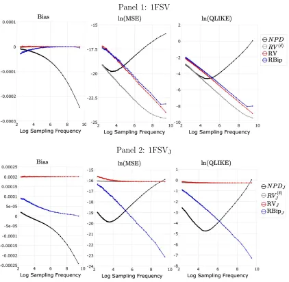
1.5 Simulated Bias, MSE and QLIKE for daily volatility estimates obtained from NPD, RV(δ), RV and RBip for 1FSV model without noise and price discretization . . . 38
1.6 Average sampling frequency of the NPD estimator for the 1FSV and 1FSVJ models . . . 40
1.7 Simulated Bias, MSE and QLIKE for daily volatility estimates obtained from NPD, RV(δ), RV and RBip for 1FSV model with moderate level of MMS noise . . . 41
1.8 Average correlogram of calendar time returns and price duration returns 42 1.9 Average sampling frequency of the NPD and NPDz estimator for the 1FSV and 1FSVJ models under optimal γ . . . 44
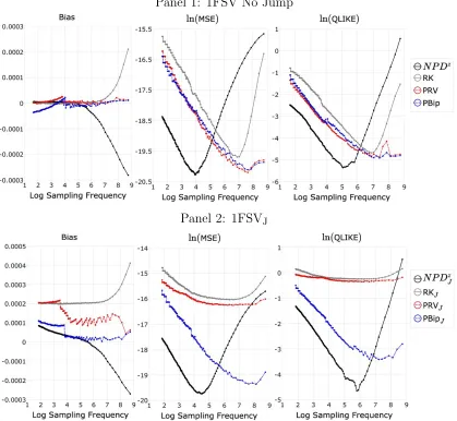
1.10 Simulated Bias, MSE and QLIKE for daily volatility estimates obtained from NPDz, RK, PRV and PBip for 1FSV model with moderate level of MMS noise . . . 45
2.1 Daily price change threshold δ for all thirty stocks from 2011-Jan to 2014-Dec . . . 66
2.2 An example of the price duration process . . . 67
2.3 Correlogram and histogram of log price durations for SPY . . . 67
2.4 Estimated diurnal patterns from models in Table 2.5 . . . 73
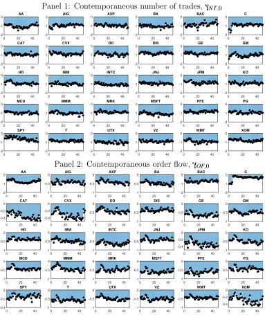
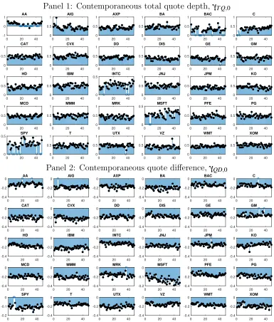
2.5 Summary of estimated contemporaneous MMS parameters of the LL-ACD(1,1)-K model for all stock-months, part 1 . . . 75
List of Figures | xv
2.7 Summary of estimated contemporaneous MMS parameters of the LL-ACD(1,1)-K model for all stock-months, part 3 . . . 77 2.8 Example of intraday volatility estimates based on ICV and RK for SPY 82 2.9 Tick-by-tick price change for SPY on 09-Aug-2011 . . . 83 2.10 15-minute volatility estimates for AA and SPY on 29-Mar-2013 . . . 86
3.1 Convergence Diagram for Spec. 1 in Table 3.1 . . . 115 3.2 Scatter plots with regression line for AIG 2016-03, INTC 2016-08, SPY
2016-05 . . . 120 3.3 R2 Difference for the volume-duration regressions in the first hour of
the day and the rest of the day . . . 121 3.4 Distribution of estimated regimes over time for AIG 2016-03, INTC
2016-08 and SPY 2016-05 . . . 124 3.5 Scatter plots with regression line for AIG 2016-03, INTC 2016-08, SPY
2016-05 based on estimated regimes . . . 125 3.6 R2 difference for the volume-duration regressions between observations
in regime 1 and 2 using the estimated state vector . . . 126
A.1 Simulated volatility signature plot for the NPD estimator on the GST model with no MMS noise . . . 158 A.2 Simulated volatility signature plot for the NPD estimator on the GST
model with i.i.d. MMS noise . . . 159 A.3 Simulated volatility signature plot for the NPD estimator on the GST
model with AR(1) MMS noise . . . 160 A.4 Simulated volatility signature plot for the NPD estimator on the GST
model with AR(1) MMS noise and price discretization . . . 161 A.5 Simulated volatility signature plot for the NPD estimator on the GST
model with price discretization and jumps . . . 162 A.6 Optimal θs of PRV and PBip estimators . . . 164 A.7 Simulated Bias, MSE and QLIKE for daily volatility estimates obtained
from NPD, RV(δ), RV and RBip for 1FSV model with high level of
MMS noise . . . 166 A.8 Simulated Bias, MSE and QLIKE for daily volatility estimates obtained
from NPD, RV(δ), RV and RBip for 1FSV model with low level of
MMS noise . . . 167 A.9 Simulated Bias, MSE and QLIKE for daily volatility estimates obtained
A.10 Simulated Bias, MSE and QLIKE for daily volatility estimates obtained from NPDz, RK, PRV and PBip for 1FSV model with low level of MMS noise . . . 169
B.1 Correlogram and histogram of log price durations for IBM, JPM and PFE . . . 182 B.2 Summary of estimated dynamic parameters of the LL-ACD(1,1)-K
model for all stock-months, part 1 . . . 183 B.3 Summary of estimated dynamic parameters of the LL-ACD(1,1)-K
model for all stock-months, part 2 . . . 184 B.4 Summary of estimated one-duration lagged MMS parameters of the
LL-ACD(1,1)-K model for all stock-months, part 1 . . . 185 B.5 Summary of estimated one-duration lagged MMS parameters of the
LL-ACD(1,1)-K model for all stock-months, part 2 . . . 186 B.6 Summary of estimated one-duration lagged MMS parameters of the
LL-ACD(1,1)-K model for all stock-months, part 3 . . . 187 B.7 Comparison betweendL and dO for all stock-months . . . 189 B.8 Correlograms and quantile-quantile plots of the estimated residuals
from model estimations in Table 2.5 . . . 191 B.9 Example of daily volatility estimates based on ICV and RK for SPY . 197 B.10 Illustration of the boundary problem of the intraday ICV estimator . 202
C.1 Examples of Deseasonalization: Raw and Deseasonalized Price Dura-tion and Volume from AIG 2016-03, INTC 2016-08, SPY 2016-05 . . 209 C.2 Lomb-Scargle Periodogram for Raw and Deseasonalized Price
Dura-tions, Volume and Bid-Ask Spread Covariates for AIG 2016-03, INTC 2016-08, and SPY 2016-05 . . . 210 C.3 Monthly choices of δ for 10-by-12 stock-month datasets . . . 225 C.4 Yearly distribution of estimated regimes over time for all stock-months
for the MS(2)-ACI(2,1)-V model . . . 225 C.5 Difference in the estimated bˆ1s from the volume-duration regressions
between observations in regime 1 and 2 using the estimated state vector226 C.6 EstimatedSoR for MS(2)-ACI(2,1) and MS(2)-ACI(2,1)-V models . . 226 C.7 Yearly distribution of estimated regimes over time for all stock-months
for the MS(2)-ACI(2,1) model . . . 227 C.8 Quantile-Quantile Plots of the residuals obtained from ACI(2,1),
List of Figures | xvii
C.9 Correlograms of the residuals obtained from ACI(2,1), ACI(2,1)-V, MS(2)-ACI(2,1) and MS(2)-ACI(2,1)-V models for AIG 2016-03, INTC 2016-08 and SPY 2016-05 . . . 229 C.10 Bayesian Information Criterion of ACI(2,1), ACI(2,1)-V, MS(2)-ACI(2,1)
and MS(2)-ACI(2,1)-V models for all stock-months . . . 230 C.11 Distribution of estimated regimes over time from the
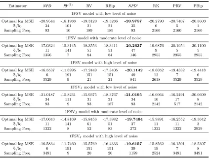
1.1 List of all volatility estimators considered in the simulation study . . 33 1.2 Comparison of the optimal MSEs for all volatility estimators in Table
1.1 for the 1FSV and 1FSVJ models with low, moderate and high
levels of noise . . . 47
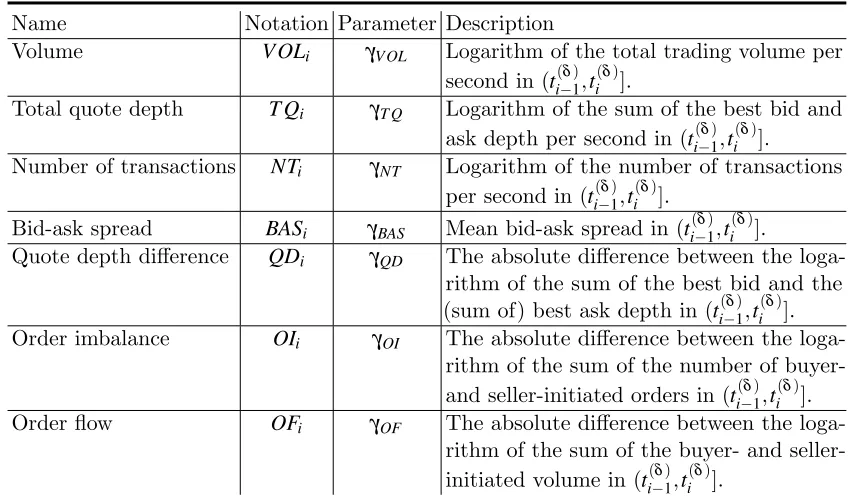
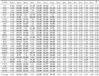
2.1 Description of MMS variables . . . 62 2.2 Cross-correlation table between log price durations and MMS covariates 68 2.3 Best-subset regression outputs for SPY, 2011-01 . . . 69 2.4 Average of monthly relative importance of MMS covariates . . . 70 2.5 Examples of LL-ACD(1,1) estimation outputs for 2011-01, SPY . . . 72 2.6 Out-of-sample performance of the LL-ACD(1,1) models . . . 80 2.7 Averaged correlation table of RK and monthly estimated intraday
ICV volatility estimates for SPY . . . 84 2.8 Comparison of MSEs of intraday ICV volatility estimates . . . 84
3.1 Monte Carlo Simulation Results of Parameter Estimates of MS(2)-ACI(1,1) Models and the Corresponding Complete Models for 100 Random Draws of Data . . . 113 3.2 Monte Carlo Simulation Results of Parameter Estimates of a
MS(3)-ACI(1,1) Model and its Complete Version for 100 Random Draws of Data . . . 115 3.3 Yearly Descriptive Statistics forx˙δ
i,d and lnVol˙ δ
i,d . . . 119 3.4 Parameter Estimates of MS(2)-ACI(2,1)-V Model for AIG 2016-03,
INTC 2016-08 and SPY 2016-05 . . . 123
A.1 Simulated moments for D˜(·) and Ri(·) and the simulated ρ(·) . . . 155 A.2 Comparison of the optimal QLIKEs for all volatility estimators in
Table 1.1 for the 1FSV and 1FSVJ models with low, moderate and
high levels of noise . . . 165
List of Tables | xix
B.2 Daily descriptive statistics of the transaction data . . . 174
B.3 Descriptive statistics of the dataset . . . 175
B.4 Descriptive statistics of the dataset . . . 176
B.5 Average of quarterly rankings of relative importance of MMS covariates177 B.6 Average of half-yearly rankings of relative importance of MMS covariates178 B.7 Average of yearly rankings of relative importance of MMS covariates . 179 B.8 Average MMS parameter estimates for the LL-ACD(1,1)-K model . . 180
B.9 Average MMS parameter estimates for the LL-ACD(1,1)-A model . . 181
B.10 Summary of diagnostic test results . . . 192
B.11 Average adjusted R-squared for models with varying estimation windows194 B.12 Summary of likelihood ratio test results . . . 195
B.13 Averaged correlation table of RK and monthly estimated daily ICV volatility estimates . . . 198
B.14 Comparison of MSEs of ICV volatility estimates within each estimation window . . . 199
B.15 Comparison of MSEs of ICV volatility estimates across different esti-mation windows . . . 200
C.1 Yearly Descriptive Statistics for xδ i,d and lnVoli,dδ . . . 219
C.2 Comprehensive estimation outputs for AIG 2016-03 . . . 220
C.3 Comprehensive estimation outputs for INTC 2016-08 . . . 221
C.4 Comprehensive estimation outputs for SPY 2016-05 . . . 222
C.5 Summary of Cram´er-von-Mises, Andersen-Darling and Ljung-Box test results . . . 223
C.6 Estimation Outputs of MS(3)-ACI(2,1)-V model for AIG 2016-03, INTC 2016-8 and SPY 2016-05 . . . 224
Introduction
Volatility estimation is an important topic in the field of finance and financial econo-metrics, as it is a crucial input for asset pricing, portfolio allocation, risk management, etc. The availability of high-frequency data recently has led to a shift from volatility modelling at low frequency (e.g the GARCH model by Engle (1982) and Bollerslev (1986) and its extensions) to high-frequency volatility measures. Since the seminal work of Andersen, Bollerslev, Diebold, and Ebens (2001) and Andersen, Bollerslev, Diebold, and Labys (2001), the Realized Volatility (RV)-type measures are popu-larized and became one of the most widely applied high-frequency volatility measures.
The popularization of the RV estimator is not surprising, as it possesses many desired properties of a volatility measure. Firstly, it is very easy to construct, as it only involves summing up squared intraday returns sampled at equidistant intervals. Secondly, assuming the log-price process to be a continuous semimartingale, the RV measure converges to the integrated variance of the price process with well-established asymptotic properties (see e.g. Barndorff-Nielsen and Shephard (2002)). Thirdly, a large number of extensions to the RV estimator are developed to address the issue that the RV measure is biased in the presence of observation errors and price discontinuities (jumps). For example, in order to correct for the bias introduced by market microstructure (MMS) noise, Zhang, Mykland, and A¨ıt-Sahalia (2005) and Zhang (2006) advocate the use of subsampling and more than one sampling frequency, Hansen and Lunde (2006) and Barndorff-Nielsen, Hansen, Lunde, and Shephard (2008a) popularize the Realized Kernel estimator, and Jacod, Li, Myk-land, Podolskij, and Vetter (2009) and Hautsch and Podolskij (2013) propose a pre-averaging approach. Examples of jump-robust RV-type estimators can be found in Barndorff-Nielsen and Shephard (2003) and Andersen, Dobrev, and Schaumburg (2012).
construction of RV measures. These two problems arise due to the non-parametric nature of the RV-type estimators, and confine the use of the RV-type estimators in situations where the amount of data is limited, i.e. less frequently traded stock or intraday volatility estimation, or incorporating other observable information in high-frequency volatility estimation.
An alternative high-frequency volatility estimator that has the potential to overcome the above problems is the point process based volatility estimator initially proposed by Engle and Russell (1998), and developed by Gerhard and Hautsch (2002), Tse and Yang (2012) and Nolte, Taylor, and Zhao (2018). As Tse and Yang (2012) summarize, this estimator enjoys a full parametric design, thus one can use data beyond the window of volatility estimation to improve the quality of parameter estimates which in turn leads to more precise volatility estimation. The parametric structure also facilitates the inclusion of other MMS covariates, which can not only further improve the quality of volatility estimation, but also provide a framework to analyse the relationship between volatility and other MMS covariates on a high-frequency level. These two properties are the key advantages of this estimator over the RV approach, and evidence also supports the superior performance of this estimator over the RV approach. Via simulation, Tse and Yang (2012) show that the point process based volatility estimator is more efficient than the RV-type estimators, and Nolte, Taylor, and Zhao (2018) find that it has better forecasting performance than the RV-type estimators. However, this estimator did not receive equal attention as the RV-type estimators, partly due to the fact that its theoretical properties are largely unknown.
This thesis is motivated by the potential of the point process based approach and attempts to popularize this approach for wider applications. The thesis consists of three individual chapters which contribute to the existing literature from both theoretical and empirical perspectives. More importantly, the thesis aims to advocate the use of the point process based approach by demonstrating that this approach is superior to the RV approach in both quality of volatility estimation and the provision of a powerful framework for MMS studies involving high-frequency volatility.
| 3
renewal process in business time under some mild assumptions. Asymptotic results can be derived based on the renewal process in business time. Our theoretical findings suggest that, firstly, the non-parametric point process based volatility estimator is more efficient than existing RV-type estimators, and the RBV approach has the po-tential to outperform RV-type estimators under any sampling scheme. Secondly, we corroborate the advantages of using a parametric structure over the non-parametric estimators such as the RV. Specifically, by augmenting the RBV estimators with a parametric structure, the efficiency of volatility estimates can be further improved without increasing the resolution of price process. This chapter provides a theoretical foundation for the point process based volatility estimators in Tse and Yang (2012) and Nolte, Taylor, and Zhao (2018), which will also be implemented in Chapters 2 and 3 of this thesis.
In addition to the theoretical considerations discussed above, Chapter 1 also provides an in-depth analysis of the Non-Parametric Duration (NPD) based volatility estimator by Nolte, Taylor, and Zhao (2018) in the presence of market frictions and jumps. We quantify the effect of jumps, time discretization, MMS noise and price discretization on theNPDestimator by a comprehensive simulation study. In our simulation results, we demonstrate that the NPD estimator is indeed more efficient than calendar time RV estimators sampled equally frequently when the sampling frequency is low, and is very robust to jumps. However, as the sampling frequency increases, the NPD estimator is more sensitive to MMS noise and thus more biased compared to the calendar time RV estimators. To overcome this problem, we propose an exponentially smoothed NPD estimator and show that it can mitigate the MMS noise bias and has the potential to outperform common noise robust RV-type methods such as the Realized Kernel and the pre-averaged RV.
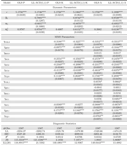
In Chapter 2, we focus on exploiting information in the MMS covariates to im-prove the quality of high-frequency volatility estimation with the point process based approach, which is a feature that is not supported by the traditional RV approach. In detail, we include trading volume, bid-ask spread, total quote depth, quote depth difference, number of trades, order imbalance and order flow in a log specification of the Autoregressive Conditional Duration (ACD) model (Engle and Russell, 1998) to construct daily and intraday volatility estimates. We implement a Best Subset Regression (BSR) approach to assess the relative importance of each variable and select the optimal number of variables.
empirical findings suggest that, firstly, the inclusion of MMS covariates can to a great extent improve the goodness-of-fit of the parametric model, and the BSR approach can effectively select the most relevant variables to include in the ACD model. This result is further reflected in the quality of daily and intraday volatility estimates. Using the Realized Kernel measure as a benchmark, we show that the inclusion of optimally selected MMS covariates significantly reduces the distance between the volatility estimates from the ACD models and the benchmark on both daily and intraday levels, and including all MMS covariates does not further improve the result. More importantly, we demonstrate that with the inclusion of MMS covariates, we can construct reliable intraday volatility estimates, even when the amount of data is considered inadequate for a reliable RV-type estimator to be constructed. Therefore, our results in the second chapter provide empirical evidence supporting the theoretical findings in Chapter 1.
In Chapter 3, we develop the Markov-Switching Autoregressive Conditional In-tensity (MS-ACI) model by extending the ACI model originally proposed by Russell (1999) with a Markov-switching structure. We augment the stationarity condition of the ACI and MS-ACI model, and show that the MS-ACI model can be reliably estimated by the Stochastic Approximation Expectation Maximization (SAEM) al-gorithm (Celeux, Chauveau, and Diebolt, 1996; Celeux and Diebolt, 1992). Our results contribute to the literature by providing a frequentists’ method to solve the path dependency problem in estimating the Markov-switching autoregressive models without any simplification to the parametric structure of the model.
| 5
on the market index, and this suggests that what we capture may be associated with firm-specific information arrivals into the market. Based on our empirical investigation, we propose to use the posterior probability of regime classification as a measure of intraday informativeness of the market.
Chapter 1
Asymptotic Theory for Renewal
Based High-Frequency Volatility
Estimation
1.1
Introduction
Since the seminal paper by Engle and Russell (1998), a point process based high-frequency volatility estimator provides an important alternative to the Realized Volatility (RV)-type estimator as popularized by Andersen, Bollerslev, Diebold, and Labys (2001). The main argument supporting the point process based volatility estimator is its parametric structure and ability to provide intraday inference on local volatility, as opposed to an integrated volatility estimator from the RV estimator. The quality of volatility estimates from point process based estimators has be verified by Tse and Yang (2012) and Nolte, Taylor, and Zhao (2018). In these papers, Tse and Yang (2012) show that the volatility estimates from fitting an Autoregressive Conditional Duration (ACD) (Engle and Russell, 1998) to the absolute price change point process can outperform RV-type estimators under the assumption of various stochastic volatility models. With the same volatility estimator, Nolte, Taylor, and Zhao (2018) show that volatility estimates from the point process can provide better predictability compared to those from the RV and RV variants. Despite these promis-ing results showpromis-ing a clear advantage of the point process based volatility estimators over the RV-type estimators, its theoretical properties have not yet been established.
volatility. They demonstrate that the duration-based volatility estimator can easily outperform the RV-type estimator in ideal conditions with a smaller mean squared error (MSE). Much of the theoretical properties of these non-parametric estimators have been discussed in these papers respectively, but none of them generalize the properties of these non-parametric estimators to a setting where both time-varying volatility and a general market microstructure noise (MMS) are present. Moreover, the duration based approach suffers from a truncation bias, when the price change is not exactly the value of the threshold. Together with the market microstructure noise, the consistency and asymptotic behaviour of these non-parametric estima-tors are largely unknown, which greatly hinders their applications in empirical studies.
We propose a general class of volatility estimators that we will refer to as the Renewal Based Volatility (RBV) estimators, which provides a theoretical framework for the aforementioned point process based volatility estimators (with the exception of the estimators in Andersen, Dobrev, and Schaumburg (2008)). This class of volatility estimators is constructed based on a renewal process in business time, which is a time change that treats the integrated variance as a measure of time. Based on this renewal process and the fact that the counts of events are shared by both business and calendar clocks, we can construct an estimator that estimates the time elapse in business time, which corresponds to the integrated variance in calendar time. As we do not require any knowledge about the dynamics of the volatility process, this estimator is by construction non-parametric. Moreover, we show that, by specifying a dynamic structure on the observed point process in the calendar time and defining a link function that maps the durations in calendar time to its counterparts in business time, one can construct parametricRBV-class estimators that can achieve a higher efficiency than their non-parametric counterparts. This includes the parametric duration-based volatility estimator as in Engle and Russell (1998), Tse and Yang (2012) and Nolte, Taylor, and Zhao (2018), and the intensity-based volatility estimator (Gerhard and Hautsch, 2002; Li, Nolte, and Nolte, 2018c). We derive the asymptotic distribution of both the non-parametric and parametric RBV estimators, and show that they are consistent as long as one can construct a renewal process in business time. One desirable property of this class of estimators is that, the asymptotic variance can be constructed without another estimation step (such as the estimation of integrated quarticity in the RV framework, see e.g. Barndorff-Nielsen and Shephard (2004)), which allows one to construct more precise confidence bounds.
1.1 Introduction | 9
We formalize the properties of theNPDestimator for a general semimartingale setting in the presence of jumps, time-varying volatility, irregular arrivals of observations, price discretization and MMS noise. Our findings suggest that, firstly, the NPD esti-mator is more robust to jumps than a realized bipower variation estiesti-mator. Secondly, although the NPD estimator has a smaller asymptotic variance than the calendar time RV-type estimators in the absence of noise, it is very sensitive to MMS noise. Consequently, theNPD estimator will be biased upwards more heavily compared to a calendar time RV-type estimators of similar sampling frequency, which significantly weakens its relative performance.
By correcting the biases for theNPD estimator and exploiting its smaller asymptotic variance, we propose to construct the NPD estimator on the exponentially smoothed price process, which we will refer to as the exponentially smoothed NPD estimator, denoted byNPDz. In our simulation we show that, if the smoothing parameter is cho-sen optimally, the truncation bias due to time discretization can approximately offset the smoothed MMS noise bias at moderate to large sampling frequencies. At these sampling frequencies, the NPDz estimator exhibits a significantly higher efficiency compared to the commonly used bias corrected calendar time sampling volatility estimators, including the Realized Kernel (Barndorff-Nielsen, Hansen, Lunde, and Shephard, 2008a), the pre-averaged RV and pre-averaged bipower variation (Hautsch and Podolskij, 2013) estimators. Additionally, we demonstrate that, although the optimal sampling frequency of theNPDz estimator is much smaller than its calendar time competitors, its optimal efficiency is still better than the optimal performance from its competitors, which requires a much larger sampling frequency.
The rest of the chapter is structured as follows: Section 1.2 describes the gen-eral theory for the renewal process and renewal reward process. Section 1.3 and 1.4 introduces the renewal based volatility estimator and the parametric renewal based volatility estimator respectively. Section 1.5 gives some examples on both the non-parametric and parametric estimators that belong to the class of renewal based estimators. In Section 1.6, we examine the NPD estimator under a general semi-martingale in the presence of various market imperfections. We conduct a Monte Carlo simulation study in Section 1.7. Section 1.8 concludes.
1.2
Prerequisites: Renewal Theory
This section summarizes the related renewal theory used in constructing the renewal based volatility estimator. For a more comprehensive discussion, please refer to standard point process textbooks, e.g. Wolff (1989), Ross (1996), etc.
We start with the definition of a renewal process:
Definition 1.1. Renewal Process: Let {Di}i=1,2,··· be a sequence of positive i.i.d.
random variables with 0<µ =E[Di]<∞ which represents the inter-event arrival
time, and let ti denote the arrival time of the i-th event (renewal epoch) given by:
ti= i
∑
j=1
Dj. (1.1)
A renewal process X(t) is defined as a random variable that counts the number of event arrivals in the interval (0,t]:
X(t)≡ ∞
∑
i=1
1l{t
i≤t}. (1.2)
A renewal process has the following asymptotic properties:
Theorem 1.1. Elemental Renewal Theorem: Let X={X(t)}t≥0 be a renewal
process with mean inter-arrival time 0<µ <∞ and renewal function m(t) =E[X(t)], then
lim
t→∞
X(t) t
a.s.
→ 1
µ, (1.3)
lim
t→∞
m(t)
t →
1
1.2 Prerequisites: Renewal Theory | 11
Proof. See e.g. Feller (1941), Doob (1948) Theorem 3.3.4, Chapter 3 in Ross (1996).
A seemingly trivial result from the above theorem is that for a given 0<µ<∞, limt→∞X(t)→∞. The renewal function, m(t) =E[X(t)], has the following second
order asymptotic expansion ast →∞:
Proposition 1.1. Let X(t) be a renewal process defined in Definition 1 with mean and variance of the inter-event arrival time denoted as 0<µ <∞ and 0<σ2<∞ respectively. Let m(t) =E[X(t)] denote the renewal function. The process m(t) has the following asymptotic expansion as t→∞:
m(t) = t µ +
σ2
2µ2−0.5+o(1). (1.5)
Proof. E.g. Corollary 3.4.7 in Ross (1996)
It is useful to consider the distribution of time elapses since the last renewal epoch. This is known as the age process of a renewal process, formally defined as follows:
Definition 1.2. Age Process of A Renewal Process: LetX(t)denote a renewal process defined in Definition 1.1. The age process of a renewal process is defined as:
A(t) =t−tX(t) (1.6)
The moments of A(t)can be derived from the moments of the renewal process if they exist:
Theorem 1.2. For an age process A(t) defined in Definition 1.2, and let the n-th moments of the inter-epoch duration of the underlying be denoted by E[Dni] =µn.
Provided that all µn exist, the moments of the age process A(t) can be expressed as:
E[An(t)] = µn+1
(n+1)µ (1.7)
Proof. See, e.g. Coleman (1982).
We will also use the property of a renewal reward process, which is defined as follows:
v<∞and variance σr2<∞associated with each Di. Then the renewal reward process
is defined as:
R(t) = X(t)
∑
i=1
Ri. (1.8)
The expectation of this process, r(t) =E[R(t)], is defined as the reward function.
A renewal reward process has the following asymptotic properties:
Theorem 1.3. Renewal Reward Theorem: For a renewal reward process defined in Definition 1.3, the following results hold:
lim
t→∞
R(t) t
a.s.
→ v
µ, (1.9)
lim
t→∞
r(t)
t →
v
µ. (1.10)
Proof. E.g. Theorem 3.6.1, Chapter 3 in Ross (1996).
1.3
Renewal Based Volatility Estimator
We are now in the position of constructing the renewal based volatility (RBV) estimator for financial price processes. We start with an assumption about the price process and the associated volatility process of interest:
Assumption 1.1. Price Processes: Let the log price process{P(t)}t>0be a
stochas-tic process with an adapted, c`adl`ag and strictly positive integrated variance (IV) process defined by IV(0,t) =Rt
0σp2(s)ds with IV(0,t)→∞ ast→∞. We define a time change τ(t) =IV(0,t) that converts the calendar time to the integrated variation time, which
is also known as the business time. We assume that the time changed price process ˜
P(τ(t)) =P(t) is a L´evy process in business time.
In the above assumption, we do not need to specify a particular form for the processσp(t)as long as it satisfies Assumption 1.1. In this section we will assume that the complete trajectory ofP(t)can be observed, and the effect of discrete observation of the price process will be analysed in Section 1.6.
We can reverse the time change t7→τ(t) by using t=inf{u∈R+:IV(0,u)≥τ(t)}. It is clear that τ(t) is a stopping time for anyt. Also, the time changed information set has the relationship Ft =F˜τ(t). For a more rigorous discussion on the change of
1.3 Renewal Based Volatility Estimator | 13
Assumption 1.1 may seem strict, but it is satisfied by a wide range of stochas-tic processes that are used in modelling financial price processes. We give two simple examples.
Example 1: Any continuous local martingale satisfies this assumption due to to following theorem.
Theorem 1.4. (Dambis-Dubin Schwarz): Let (M(t))t≥0 be a continuous Ft
-local martingale such that its quadratic variation ⟨M⟩∞= +∞, then there exists a
Brownian motion (B(t))t≥0, such that for everyt ≥0, M(t) =B(⟨M⟩t).
Since the quadratic variation and integrated variance of M(t) coincide, the result-ing L´evy process in business time is a standard Wiener process. Note that Theorem 1.4 still holds when the stochastic volatility and the price process are correlated, which is known as the ‘leverage effect’ that is commonly observed in practice (see e.g. Bollerslev, Litvinova, and Tauchen (2006)).
Example 2: A (inhomogeneous) compounded Poisson process as in Oomen (2005) satisfies this assumption. The resulting L´evy process is a homogeneous compounded Poisson process. See Appendix A.1 for details. 1
The connection from the L`evy process in business time and the renewal theory in the previous section is established by the following proposition:
Proposition 1.2. Let {Y(t)}t≥0 be a L´evy process on the filtered probability space {Ω,F,P}. Define a stopping time process that automatically renews once stopped as:
ti= inf
t≥ti−1
{Y(t)∈S(ti−1)}, (1.11)
in whichS(ti)is the stopping condition for ti as a function ofFti. If, for anyi,j and
t >0, Prob(Y(ti+t)∈S(ti)) =Prob(Y(tj+t)∈S(tj)), then the sequence {ti}i=1,2,···
corresponds to arrivals of a renewal process.
Proof. The condition Prob(Y(ti+t)∈S(ti)) =Prob(Y(tj+t)∈S(tj)) ensures that the stopping condition is equivalent to the paths of the L´evy process originating from all the possible starting points ti∈(0,∞) regardless of when the previous event
occurred. Then clearly the distribution of ti−ti−1 is i.i.d., which follows from the property of the L´evy process. As a result, {ti}i=1,2,··· is by definition a renewal
process.
1Relying on Theorem 1.4, we can account for the leverage effect if the latent price process follows
Consequently, when the price processP(t)follows Assumption 1.1, we can obtain a L`evy processP˜(τ(t))in business time. According to Proposition 1.2, we can construct a renewal process {τ(ti)}i=1,2,··· in business time by choosing an appropriateS(τ(ti)) for each i. Effectively, we sample the price process at{ti}i=1,2,··· in calendar time in
such way that the business time counterpart {τ(ti)}i=1,2,··· is renewal. We therefore
refer to this sampling scheme as renewal sampling:
Definition 1.4. Renewal Sampling: For a price process P(t) satisfying Assump-tion 1.1, a renewal sampling scheme samples P(t) at 0<t1 <t2 <· · · where the arrivals in business time {τ(ti)}i=1,2··· is a renewal process in business time. Denote
the unobservable renewal process in business time as X˜(τ(t)) =∑i>01l{τ(ti)≤τ(t)} and
its observable calendar counterpart as X(t) =∑i>01l{ti≤t}.
Note that the c`adl`ag property of the integrated variance guarantees that X(t) =
˜
X(τ(t)). Using Proposition 1.2, we can constructX(t)in calendar time if the stopping condition in calendar time is only a function of the paths of P(t), but not a function of time. Heuristically, by observing the path of the price process in calendar time, we can decide where to ‘stop’ the price process and obtain a sample. If the condition in Proposition 1.2 for S(ti) is satisfied, then the stopping times in business time is by construction a renewal process.
The central contribution of this chapter is the following novel volatility estimator by sampling the price process P(t) with a renewal sampling scheme:
Definition 1.5. Renewal Based Volatility (RBV) Estimator: Let {P(t)}t>0 be
a price process that satisfies Assumption 1.1. Choose a S(ti) according to Propo-sition 1.2, and apply renewal sampling on P˜(τ(t)) to obtain the renewal sampling times {ti}i=1,2,··· and the point process X(t) =∑i>01l{ti≤t}, which has a business time
counterpart X˜(τ(t)) that is a renewal process. Let 0<µ<∞ and 0<σ2<∞ denote the first two moments of the inter-epoch duration in business time, then the RBV
estimator is defined by:
RBV(0,t) =X(t)µ. (1.12)
The RBV estimator has the following asymptotic distribution:
Theorem 1.5. The Renewal Based Volatility estimator as defined in Definition 1.5 has the following asymptotic distribution:
lim
t→∞
RBV(0,t)−IV(0,t)
p
X(t)σ
d
→N (0,1) (1.13)
1.4 Parametric Renewal Based Volatility Estimator | 15
One remark on the RBV estimator is that we can compute standard errors of the estimator without estimating the integrated quarticity as in the RV literature, which implies less estimation bias for the standard errors and confidence bounds. Similar to the RV-type estimators, theRBV estimator does not require any parametric assumption on the IV process in calendar time. The obvious problem here is that
µ is not explicitly specified, and is dependent on the assumption of P(t) and the stopping condition S(ti). In Section 1.5 we show that in some special cases µ is available in closed form. Also, the processP˜(τ(t))is usually very simple (for example, a standard Wiener process). In this case the moments of the renewal process can be simulated easily.
We would like to point out that in (1.13), the limiting distribution is obtained when µ is fixed and t→∞. This is known as the sprawl asymptotics, or the
long-span asymptotics, which is typical in the context of point processes. However, this is different to the infill asymptotics usually applied in the RV context where the time frame is fixed and the sampling frequency increases. To derive counterpart of Theorem 1.5 in the infill asymptotics setting, more assumptions are required for the asymptotic behaviour ofP(t) and X(t), which is presented in Appendix A.3.
To distinguish between the two asymptotic settings, for the rest of the chapter, the sprawl asymptotics is involved when the construction of the price durations is fixed. Consequently, the moments of the price durations in business time, namely, µ,
σ2, are fixed. Asymptotic results are derived by expanding the sampling window and lettingt→∞. For the infill case, the time span is fixed and we allow the moments of
the price durations in business time to change. Asymptotic results in this case are typically derived by letting µ →0 for a fixed time frame.
1.4
Parametric Renewal Based Volatility
Estima-tor
The duration in business time D˜i is not directly observable, but we can observe its calendar time counterpartDi. Using the fact that D˜i is i.i.d., the connection between Di and the integrated variance process is that:
Z ti−1+Di
ti−1
If we can specify a parametric model g(t|Ft) that uses all the information available in such a way that the following variable is i.i.d:
Ri=
Z ti−1+Di
ti−1
g(s|Fs)ds, (1.15)
then we can use the quantity Riµ
E[Ri] as an estimator for
˜
Di. Without any loss of generality we setE[Ri] =µ to simplify notation. We will refer to this estimator as the parametric renewal based volatility (PRBV) estimator, formally defined as follows:
Definition 1.6. Parametric Renewal Based Volatility (PRBV) Estimator:
Let{P(t)}t>0, X(t), X˜(τ(t)), µ and σ2be defined identically to Definition 1.5. Define
a parametric model g(t|Ft) and an i.i.d. variable Ri that follows (1.15) with 0<
E[Ri] =µ <∞ and 0<V[Ri] =σr2<∞. Then the PRBV estimator is defined as:
PRBV(0,t) = X(t)
∑
i=1 Ri=
Z t
0
g(s|Fs)ds. (1.16)
Recall that the RBV estimator is already consistent, therefore for any i.i.d. Ri with finite moments, the PRBV estimator will still be consistent. However, the randomness in Ri may introduce extra noise in the PRBV estimator, unless there exists a substantial amount of positive correlation between Ri and D˜i, which requires that g(t|Ft) is a good proxy of σp2(t) for allt. Thus, we can assess the efficiency of the PRBV estimator by using theRBV estimator as a benchmark.
Conditioning on that we can observe the i.i.d. variable Ri, the asymptotic dis-tribution of the PRBV estimator can be derived analogously to the derivation of Theorem 1.5 noting that Ri−D˜i is a zero-mean i.i.d. variable, and the pair {Ri,D˜i}
forms a renewal reward process.
Theorem 1.6. The Parametric Renewal Based Volatility estimator as defined in Definition 1.6 has the following asymptotic distribution:
lim
t→∞
PRBV(0,t)−IV(0,t)
p
X(t)(σ2+σ2
r −2ρ σ σr) d
→N (0,1) (1.17)
where ρ is the correlation between Ri and D˜i.
Proof. This follows similarly from the proof in Appendix A.2 by using that the variableRi−D˜i is i.i.d. with zero mean. Note thatV[Ri−D˜i] =σ2+
σr2−2ρ σ σr.
1.4 Parametric Renewal Based Volatility Estimator | 17
is known. The variance of the PRBV estimator can be written as:
V[PRBV(0,t)] =V[RBV(0,t)] +X(t)(σr2−2ρ σ σr), (1.18)
and as long as σr2−2ρ σ σr<0, that is, ρ ∈(2σσr,1], the PRBV estimator will always be more efficient than theRBV estimator. Obviously, the value of ρ is determined by the distance between g(t|Ft) and σp2(t), which is unfortunately model dependent.
We provide an example of g(t|Ft) which allows us to examine ρ directly. Initially proposed by Gerhard and Hautsch (2002) derived from the instantaneous volatility estimator of Engle and Russell (1998), the conditional intensity process of X(t) is used as a proxy of the instantaneous volatility. We defineg(t|Ft) as follows:
g(t|Ft) =µ λ(t|Ft), (1.19)
where λ(t|Ft) is theFt-conditional intensity of the process X(t) defined as:
λ(t|Ft)≡lim
∆↓0
1
∆E[
X(t+∆)−X(t)|Ft]. (1.20)
The corresponding renewal reward variable Ri is then defined as:
Ri=µ
Z ti
ti−1
λ(s|Fs)ds≡µΛ(ti−1,ti). (1.21) The i.i.d.-ness of Ri is guaranteed by the following theorem:
Theorem 1.7. Random Time Change Theorem (RTCT): LetX(t) be a simple point process adapted to a history Ft with bounded, strictly positive Ft-conditional intensity λ(t|Ft) and Ft-compensators Λ(t) =
Rt
0λ(u|Fu)du with Λ(∞) =∞ almost
surely. Under the random time change t7→Λ(t), the transformed process
˜
X(t) =X(Λ−1(t)) is a Poisson process with unit rate.
Conversely, suppose there is given a history Gt, a Gt-adaptive cumulative process
M(t) with a.s. finite, monotonically increasing and continuous trajectories, and a
Gt-adapted simple Poisson process X0(t). Let Ft denote the history of σ-algebras
Ft=GM(t). Then X(t) =X0(M(t)) is a simple point process that is Ft-adapted and
has Ft-compensator M(t).
Theorem 1.7 suggests thatΛ(ti−1,ti)∼i.i.d.exp(1), so we haveRi∼i.i.d.exp(µ−1). The mean and variance of Ri are v=µ and σr2=µ2 respectively. We derive the following important proposition that characterizes the relationship between the conditional intensity processes in calendar time and business time:
Proposition 1.3. LetX(t)be a simple point process with conditional intensity process
λ(t|Ft), and let t 7→τ(t) be a change of time from calendar time to business time.
The conditional intensity process λ˜(τ(t)|F˜τ(t)) of the time-changed point process ˜
X(τ(t)) follows:
˜
λ(τ(t)|F˜τ(t))σp2(t) =λ(t|Ft). (1.22)
Proof. See Appendix A.4.
Proposition 1.3 has some very powerful implications that provide theoretical foundations for intensity and duration based volatility estimation.
Corollary 1.1. In Definition 1.6 with g(t|Ft) =µ λ(t|Ft), the rank correlation
between Ri and D˜i is 1. Additionally, if D˜i is i.i.d. exponentially distributed, then
g(t|Ft) =σp2(t).
Proof. See Appendix A.5.
Corollary 1.1 suggests that, firstly, thePRBV estimator is likely to perform well due to the monotonic non-linear relationship between Ri and D˜i. Secondly, the optimal renewal sampling scheme for g(t|Ft) =µ λ(t|Ft) is a homogeneous Poisson sampling scheme in business time. In this case, the conditional intensity of X(t) in calendar time is proportional to the spot volatility, so that the conditional intensity is a perfect estimator of instantaneous volatility for allt. However, the assumption that
˜
Di is i.i.d. exponentially distributed requires further assumptions on the price process (e.g. the compounded Poisosn process in Oomen (2006)), which is not desirable.
Alternatively, we can also correct for the discrepancy between the density of D˜i and Ri:
Corollary 1.2. In Definition 1.6 with g(t|Ft) = µ λ(t|Ft), let FD˜(x) and FD−˜ 1(x)
denote the CDF of D˜i and its inverse correspondingly. The following relationship holds for all i:
˜
Di=F−˜ 1
D (1−exp(−Ri/µ)) (1.23)
1.5 Some Examples | 19
The expression F−˜ 1
D (1−exp(−Ri/µ))is effectively an exponential inverse proba-bility integral transformation of D˜i, which is a perfect estimator for the volatility between the two points (ti−1,ti]. However, this is a weaker result compared to Corol-lary 1.1 because in generalg(t|Ft)≠ σp2(t). In this case, inference based onRi only reflectsD˜i in expectation with E[Ri] =E[D˜i] with a rank correlation of 1, andg(t|Ft) does not estimate the actual spot volatility.
From above, it is clear that regardless of the value of µ, if we know the true conditional intensity process in calendar time, we in principle know the underlying integrated variance process. Therefore, in practice one does not need to sample at ultra high-frequency to improve the precision of the volatility estimates, which is the common approach in the RV literature. Instead, one only needs to append the estimation window of the econometric model of the conditional intensity process to obtain a more precise estimate of the conditional intensity, which in turn leads to a more precise estimate of D˜i for each i. This is in stark contrast with the RV-type estimators which relies heavily on the availability of data within the volatility estima-tion window. We stress that this is a very important property of the PRBV estimator that validates the intraday volatility estimates as in Engle and Russell (1998) and Tse and Yang (2012), and also renders the PRBV estimator advantageous over the RV-type estimator in the situation where the availability of data is limited.
To summarize our findings on the PRBV estimators, we have shown that, it is possible to construct a PRBV estimator as in Corollary 1.2 that always has zero variance if Ri is known. However, these properties are unlikely to hold in practice as we do not observeg(t|Ft)and have to use a model to estimate gˆ(t|Ft)andRˆi instead. This will inevitably introduce estimation noise in the model, even if the specification of g(t|Ft) is correct. As this is more related to the properties of the econometric model used for the observed point process that deserves individual investigations, we will leave it for future research.
1.5
Some Examples
We give some concrete examples of RBV and PRBV in this section and summarize their properties. Assume the efficient log-price follows a semi-martingale of the following form:
dP(t) =α(t)dt+σp(t)dW(t), (1.24)
where α(t) is a continuousFt-predictable process and σ(t)is assumed to be c`adl`ag and strictly positive with Rt
and no discontinuities in the diffusion process for simplicity, and will discuss the effect of the drift term and jumps in the next section. The quantity of interest here is the integrated variance of the process over an interval (0,T):
IV(0,T) =
Z T
0
σp2(s)ds. (1.25)
Example 1: The first example of an RBV estimator, which will also be examined
in detail in later sections, is the non-parametric duration-based (NPD) volatility estimator proposed by Nolte, Taylor, and Zhao (2018). We start by defining the absolute price change point process, firstly introduced by Engle and Russell (1998):
Definition 1.7. The Absolute Price Change Point Process: The absolute price change point process {ti(δ)}i=0,1,··· for an observed price process P(t) and a given
price change threshold δ is constructed as follows:
1. Set t0(δ)=0 and choose a threshold δ.
2. For i=1,2,· · ·, compute the first exit time, ti(δ), of P(ti(−δ1)) through the double barrier [P(ti(−δ1))−δ,P(ti(−δ1)) +δ] as:
ti(δ)= inf
t>t(i−δ)1
{|P(t)−P(ti(−δ)1)| ≥δ}.
Iterate until the sample is depleted.
The arrivals of ti(δ) are referred to as price events. In the RBV framework, we can write S(δ)(t(δ)
i ) ={P(t
(δ)
i )−δ,P(t
(δ)
i ) +δ} and clearly it satisfies the condition in Proposition 1.2. Define the time change as τ(t) =Rt
0σ2(s)ds=IV(0,t), andP(τ(t)) is a standard Brownian motion by Theorem 1.4. As a result from Theorem 1.2, under business time, {τ(ti(δ))}i=1,2,··· forms a renewal process, denoted by X(δ)(τ(t)).
Let D(iδ) =ti(δ)−ti(−δ1) and D˜i(δ) =τ(ti(δ))−τ(ti(−δ1)) denote the duration under cal-endar time and business time respectively. Note that D˜(iδ) is the stopping time for a Wiener process (starting at zero) to exit a symmetric interval [−δ,δ]. We can retrieve its moments from its moment generating function (see Table 1 in Andersen, Dobrev, and Schaumburg (2008)). The first three moments are:
E[D˜(iδ)] =δ2, E[(D˜(iδ))2] =5
3δ
4, E[(D˜(δ)
i )
3] = 61
15δ
6. (1.26)
The NPD estimator in Nolte, Taylor, and Zhao (2018) is of the following form:
1.5 Some Examples | 21
Note we use the notation µ(δ)and σ2(δ) to denote the mean and variance of the price duration in business time for some δ. Therefore it is clear that the NPD estimator belongs to the class ofRBV estimators. The asymptotic distribution of the NPD estimator can be derived easily from (1.13):
lim
t→∞
NPD(0,t)−IV(0,t)
q
2
3X(δ)(t)δ4 d
→N (0,1) (1.28)
Using the asymptotic relationship δ2= IV(0,t)
X(δ)(t), we see that V[NPD(0,t)]→
2IV(0,t)2
3X(δ)(t). This suggests that, given a common sampling frequency, on average the NPD esti-mator will be more than six times as efficient as the RV sampled in calendar time, exactly six times as efficient as the RV sampled in business time, and more efficient than the RV under tick time sampling due to thatIV(0,t)2≤IQ(0,t) from Jensen’s inequality (Fukasawa, 2010a).
The efficiency gain from the RV estimator is not surprising. Since the NPD es-timator uses information in the path of the prices, it effectively uses more data than the RV estimator under the same sampling frequency. Additionally, as discussed in Section A.3.1, the NPD estimator is both an RBV estimator and a renewal RV estimator. It achieves the optimal efficiency for the renewal RV estimators due to the fact that the kurtosis of the return is 1.
Example 2: Inspired by Christensen and Podolskij (2007) and Andersen,
Do-brev, and Schaumburg (2008) and following the idea of theNPD estimator, we can also construct a range duration-based RBV-type volatility estimator. Let r denote a fixed range size, then the following sequence of stopping times forms a renewal process in business time:
ti(r)= inf
t>ti(−δ1)
{P(t)∈S(r)(ti(r))}, (1.29)
whereS(r)(ti(r)) ={P(t): sup
ti(r)<s<tP(s)−infti(r)<s<tP(s)≥r}. Similar to theNPD es-timator, letX(r)(τ(t))denote the renewal process under business time. The first three moments ofD˜(ir)=τ(ti(r))−τ(ti(−r)1)is as follows (Andersen, Dobrev, and Schaumburg, 2008)):
E[D˜(ir)] = 1
2r
2, E[(D˜(r)
i ) 2] = 1
3r
4, E[(D˜(r)
i )
3] =17
60r
and the non-parametric range duration-based volatility (NPR) estimator is simply:
NPR(0,t) = 1
2X
(r)r2, (1.31)
which has the following asymptotic distribution ast→∞:
lim
t→∞
NPR(0,t)−IV(0,t)
q
1
12X(r)(t)r4 d
→N (0,1) (1.32)
Using the asymptotic relationship r2= 2IV(0,t)
X(r)(t) , we have V[NPR(0,t)] =
IV2(0,t)
3X(r)(t). So the NPR estimator is twice as efficient as theNPDestimator for a common sampling frequency.
The efficiency gain of the range-based estimators compared to the RV-based es-timators has been addressed by Christensen and Podolskij (2007) and Andersen, Dobrev, and Schaumburg (2008), as price ranges exploit both the supremum and infimum of the price process, which can measure volatility more precisely than using price changes. We would like to stress that the asymptotic variance of the NPR estimator is smaller than the asymptotic variance of a general RV estimator under any sampling scheme (Fukasawa, 2010b; Fukasawa and Rosenbaum, 2012). With this
NPR example, it is clear that the RBV-class of estimators are in essence different from the RV-type estimators.
Example 3: The parametric duration (intensity) based volatility estimator, initially proposed by Engle and Russell (1998) and further developed by Gerhard and Hautsch (2002), Tse and Yang (2012), Nolte, Taylor, and Zhao (2018) and Li, Nolte, and Nolte (2018b) is an example of a PRBV estimator. Specifically, it specifies the dynamics of D(iδ) with a fully parametric model (for example, the Autoregressive Conditional Duration model by Engle and Russell (1998)), and defines
g(δ)(t|F
t) =µ λ(δ)(t|Ft) =δ2λ(δ)(t|Ft), (1.33) in which λ(δ)(t|Ft) is the conditional intensity process of X(δ)(t) defined in (1.20). Gerhard and Hautsch (2002) propose an instantaneous volatility estimator defined as InsV(δ)(t) =g(δ)(t|F
t), and an estimator of the IV between the arrival of two price
events can be constructed as follows:
R(iδ)=
Z ti(δ)
t(i−δ)1
g(s|Fs)ds=δ2Λ
(δ)
i ∼i.i.d.exp(δ
1.5 Some Examples | 23
with E[R(iδ)] =δ2 and V[R(iδ)] =δ4. As this quantity is i.i.d. from Theorem 1.7, the parametric duration (intensity) based (PD) estimator of the following form:
PD(0,t) = X(δ)
∑
i=1
R(iδ), (1.35)
is by definition a PRBV-class estimator. The asymptotic properties of the PRBV estimator discussed in Theorem (1.6) and Proposition 1.3 can be applied directly to derive the asymptotic distribution of the PDestimator:
lim
t→∞
PD(0,t)−IV(0,t)
p
C·X(δ)(t)δ4 d
→N (0,1), (1.36)
in whichC is a constant which cannot be solved analytically. From Proposition 1.3, sinceD˜(iδ) can be easily simulated based on a Wiener process, we can simulate the constantC easily. Details of this simulation can be found in Appendix A.6. Based on 1000000 replications, we found thatC≈0.034. Therefore, the asymptotic variance of the PDestimator is roughly one-twentieth of the NPD counterpart. It shows that, if the parametric model of λ(δ)(t|Ft) is well-specified, then there can be a substantial efficiency gain from the parametric estimation.
Based on the NPR estimator, we can construct a parametric range (PR) based volatility estimator by defining the renewal variable R(ir) as:
R(ir)=0.5r2
Z ti(r)
ti(−r)1
λ(r)(s|Fs)ds. (1.37)
The PR estimator is defined analogously to the PDestimator as:
PR(0,t) = X(r)
∑
i=1
R(ir)=R(r)(t), (1.38)
From the simulation in Appendix A.6 and the property of the PRBV estimator, we can derive the asymptotic distribution ofPD given R(ir):
lim
t→∞
PR(0,t)−IV(0,t)
√
C·X(r)(t)r4 d
→N (0,1), (1.39)
We would like to stress that, although the PD and PR estimators for the inte-grated variance are unbiased and consistent in the sense of expectation, using R(i·) as an estimator of D˜(i·) will introduce a non-zero error due to the discrepancy between R(i·) andD˜(i·). We plot the simulatedln(D˜(i·))againstln(R(i·))in Figure 1.1. The figure suggests that, as the discrepancy betweenR(ir) andD˜i(r) is larger than that ofR(iδ) and
˜
D(iδ), thePRestimator will be less efficient compared to thePDestimator. Also, based on the simulated D˜(i·), one can correct this discrepancy by the method in Corollary 1.2. After the correction, both estimators will have zero variance conditioning on the knowledge of R(i·).
Figure 1.1 Discrepancy between the density ofR(i·) and D˜(i·)
-3 -2 -1 0 1 2
-7.5 -5 -2.5 0 2.5
-3 -2 -1 0 1
-8 -6 -4 -2 0 2
Note: N=1000000. Descriptive statistics of{D˜(·)}
i=1:N and{R(
·)
i }i=1:N can be seen in Table A.1.
1.6 The NPD Volatility Estimator Under Market Frictions | 25
1.6
The
NPD
Volatility Estimator Under Market
Frictions
This section discusses the theoretical properties of theNPDvolatility estimator defined in (1.27) in the presence of drift, jumps, time discretization, market microstructure noise, and rounding effect.
1.6.1
Drift Effect
This section aims to clarify that the drift will not bias our estimator in an infill setting.2 As the drift effect is very small in empirical high frequency applications, we will follow the approach by Barndorff-Nielsen and Shephard (2002) and discuss the drift effect in this section and assume it to be zero in other sections.
Firstly, as discussed in previous section, the NPD estimator is also a renewal RV estimator, and the quadratic variation theory can be applied. Therefore under the as-sumption of (1.24) and asδ→0, the drift term will not bias our estimator. Moreover, we would like to note that there always exists a probability measure where the price process does not possess a drift by the use of Girsanov-Maruyama transformation. As the volatility remains unchanged after the change of measure and the NPDestimator can also be constructed on that probability measure, the presence of a drift is not a main concern under the infill setting.
1.6.2
Jump Effect
This section discusses the possible effect of jumps on the NPD estimator in the infill asymptotics setting. The NPD estimator is by construction very robust to large jumps, as pointed out by Andersen, Dobrev, and Schaumburg (2008), Tse and Yang (2012) and Nolte, Taylor, and Zhao (2018), because of its truncation feature. For simplicity, we consider the following diffusion process with jumps on the interval (0,T]:
P(t) =P(0) +
Z t
0
σp(s)dW(s) + J(t)
∑
j=1
Lj, (1.40)
where J(t) is a counting process independent of W(t), and Lj is the size of the j-th jump. We assume that |Lj−δ|>0 almost surely for all j as δ →0, so that
2Note that a drift in (1.24) can in general be estimated in the long-span asymptotics, and it will
also introduce a positive bias to theNPDestimator. We were unable to derive a bias correction