Power generation control of a monopile hydrostatic wind turbine using an H∞ loop shaping torque controller and an LPV pitch controller

warwick.ac.uk/lib-publications

Original citation:

Tong, Xin and Zhao, Xiaowei. (2017) Power generation control of a monopile hydrostatic

wind turbine using an H

∞

loop-shaping torque controller and an LPV pitch controller. IEEE

Transactions on Control Systems Technology.

Permanent WRAP URL:

http://wrap.warwick.ac.uk/92178

Copyright and reuse:

The Warwick Research Archive Portal (WRAP) makes this work by researchers of the

University of Warwick available open access under the following conditions. Copyright ©

and all moral rights to the version of the paper presented here belong to the individual

author(s) and/or other copyright owners. To the extent reasonable and practicable the

material made available in WRAP has been checked for eligibility before being made

available.

Copies of full items can be used for personal research or study, educational, or not-for profit

purposes without prior permission or charge. Provided that the authors, title and full

bibliographic details are credited, a hyperlink and/or URL is given for the original metadata

page and the content is not changed in any way.

Publisher’s statement:

“© 2017 IEEE. Personal use of this material is permitted. Permission from IEEE must be

obtained for all other uses, in any current or future media, including reprinting

/republishing this material for advertising or promotional purposes, creating new collective

works, for resale or redistribution to servers or lists, or reuse of any copyrighted component

of this work in other works.”

A note on versions:

The version presented here may differ from the published version or, version of record, if

you wish to cite this item you are advised to consult the publisher’s version. Please see the

‘permanent WRAP URL’ above for details on accessing the published version and note that

access may require a subscription.

Power generation control of a monopile hydrostatic

wind turbine using an

H

_∞

loop-shaping torque

controller and an LPV pitch controller

Xin Tong and Xiaowei Zhao

Abstract_{—We transform the NREL (National Renewable}

En-ergy Laboratory) 5-MW geared equipped monopile wind turbine model into a hydrostatic wind turbine (HWT) by replacing its drivetrain with a hydrostatic transmission drivetrain. Then we design an H∞ loop-shaping torque controller (to regulate the

motor displacement) and a linear parameter varying (LPV) blade pitch controller for the HWT. To enhance performances of the pitch control system during the transition region around the rated wind speed, we add an anti-windup (AW) compensator to the LPV controller, which would otherwise have had undesirable system responses due to pitch saturation. The LPV AW pitch controller uses the steady rotor effective wind speed as the scheduling parameter which is estimated by LIDAR (Light Detection and Ranging) preview. The simulations based on the transformed NREL 5-MW HWT model show that our torque controller achieves very good tracking behaviour while our pitch controller (no matter with or without AW) gets much improved overall performances over a gain-scheduled PI pitch controller.

Index Terms—Hydrostatic transmission, LIDAR preview, lin-ear parameter varying control, anti-windup, H∞ loop-shaping.

I. INTRODUCTION

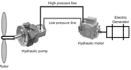
Wind power has been used as a clean source of renewable energy with sustainable growth in penetration and investments. To harvest more frequent and stronger winds, large wind turbines are being increasingly installed offshore, which are subjected to severe weather causing tremendous stress on the drivetrains. However, the gearbox of a conventional wind turbine drivetrain is very expensive and vulnerable, whose maintenance is difficult and expensive, particularly in the offshore case [1]. Replacing the gearbox drivetrain with a hydrostatic transmission (HST) one offers a more reliable solution. The latter has a much longer life cycle. A wind turbine with an HST drivetrain is called a hydrostatic wind turbine (HWT). Figure 1 (taken from Dutta [2]) represents a typical HST drivetrain. The rotor is directly coupled to a hydraulic pump in the nacelle, driving the high pressurised oil to operate a hydraulic motor which is coupled with a generator to produce electric power. The low pressure line transports the low pressure oil back to the pump from the motor. We consider the HST drivetrain with a fixed displacement pump and a variable displacement motor, which enables the HST to offer continuously variable transmission from the rotor/pump shaft speed to the motor/generator shaft speed. This allows

[image:2.612.324.555.196.320.2]

X. Tong and X. Zhao (Corresponding Author) are with the School of Engineering, University of Warwick, Coventry, CV4 7AL, United Kingdom, e-mail: [email protected]; [email protected].

Fig. 1. Main components of a typical HST drivetrain in the HWT, as well as their connections. This figure is taken from the literature [2].

the utilisation of a synchronous generator without the need for power electronics to match the grid frequency [1]. The motor & generator of the HST drivetrain can be either configured in the nacelle [2], [3] or at the tower base [4], [5]. In the present paper, we consider the former configuration, which has less operation & maintenance costs [1]. Several papers discussed the influences of different HST configurations on the turbine responses [1], [6].

To solve the above challenges, we design an H∞

loop-shaping torque controller and a linear parameter varying (LPV) pitch controller with an anti-windup (AW) compensator for the HWT. The LPV AW controller is scheduled by the steady rotor effective wind speed estimated by a LIDAR (Light Detection and Ranging) simulator. We assess both controllers based on a detailed aero-hydro-servo-elastic speed variable-pitch HWT simulation model. This model is transformed from the well-known geared equipped NREL (National Renewable Energy Laboratory) 5-MW baseline monopile wind turbine model within FAST (Fatigue, Aerodynamics, Structures, and Turbulence), through replacing its gearbox drivetrain with an HST one as shown in Fig. 1. The simulation results demon-strate that our torque controller achieves very good tracking behaviours and our pitch controller obtains much better overall performances (in regulating the rotor speed & generator power and reducing the loads on the blade bearings & tower) than the gain-scheduled PI pitch controller developed in [5].

The structure of the paper is as follows. In Section II, we transform the NREL 5-MW geared equipped monopile wind turbine model within FAST into a detailed monopile HWT. Then in Section III, we design an H∞ loop-shaping torque

controller and an LPV AW blade pitch controller for the HWT. In Section IV, we test the performances of our torque and pitch controllers through simulation studies using the transformed HWT model. Finally in Section V we conclude this paper.

II. TRANSFORMATION OF THENREL 5-MW BASELINE

MONOPILEWINDTURBINEMODEL WITHINFASTINTOA HYDROSTATICWINDTURBINE

Nowadays, monopile substructures dominate offshore wind installations [7]. The NREL 5-MW baseline monopile wind turbine model represents the current typical geared equipped wind turbine [8], which is usually simulated by the NREL FAST code [9]. Its cut-in, rated, and cut-out wind speeds are 3 m/s, 11.4 m/s, and 25 m/s, respectively. In this section, we transform the NREL 5-MW baseline monopile turbine model within FAST into a detailed aero-hydro-servo-elastic hydrostatic wind turbine (HWT) model for simulation studies, by replacing its gearbox drivetrain system with the HST drivetrain shown in Fig. 1.

We employ the HST mathematical model (2.1)–(2.3) from Laguna [5], and the parameters therein which were tailored for a simplified NREL 5-MW HWT.

˙

ωr= 1

Jr+Jp

(τaero−τp), (2.1)

˙

Dm= 1

Tm

(Dmd−Dm), (2.2)

˙

xl=Alxl+Bl1 Bl2

Qp

Qm

,

Pp

Pm

=

Cl1

Cl2

xl. (2.3)

(2.1) represents the rotational motion of the rotor/pump shaft, whereJr andJp are the moments of inertia of the rotor and pump, respectively. τaero is the aerodynamic torque which depends nonlinearly on the rotor/pump shaft speed ωr, the rotor effective wind speedV, and the blade pitch angleβ.τp is the pump torque described by

τp=DpPp+Bpωr+Cf pDpPp (2.4)

whereDpandPpare the pump displacement and the pressure difference across the pump, respectively. Bp and Cf p are the viscous damping and Coulomb friction coefficients of the pump, respectively. (2.2) describes the displacement actuator dynamics of the variable displacement motor, whereDmand

Dmd are the motor displacement and its command, respec-tively.Tm is the time constant. (2.3) represents the dynamics of the 10-m high pressure hydraulic line (assuming the low pressure line has constant pressure), with the flow rates of the pump and motor (Qp andQm) as the inputs and the pressure differences across the pump and motor (Pp and Pm) as the outputs [5], [10].Qp andQm are given by

Qp=Dpωr−CspPp, Qm=Dmωm+CsmPm, (2.5)

where Csp and Csm are the laminar leakage coefficients of the pump and motor, respectively. ωm is the fixed rotational speed of the assembly composed of the motor and synchronous generator. According to (2.5), Qm varies with the change of

Dm, which affects Pp in accordance with (2.3), and thus affectsτp (2.4). The generator power is

pg =ητmωm (2.6)

whereηis the generator efficiency andτmis the motor torque:

τm=DmPm−Bmωm+Cf mDmPm (2.7)

in whichBmandCf mare the viscous damping and Coulomb friction coefficients of the motor, respectively.

We modify the ElastoDyn input file of FAST (which contains the turbine structural information) to transform the gearbox drivetrain to the HST one. The relevant FAST DOFs are the generator DOF and drivetrain torsional flexibility DOF [9]. If we enable the former DOF and disable the latter one (assuming a rigid drivetrain shaft), the rotational motion of the rotor shaft is

˙

ωr= 1

Jr+n2Jg

(τaero−nτg) (2.8)

where n is the gearbox ratio which is 97 for the baseline turbine.Jg andτg are the generator inertia and torque. If we set n = 1 and regard the generator in the geared equipped turbine as the hydraulic pump in the HWT, then (2.8) and (2.1) are equivalent. Hence, to replace the baseline rotor shaft dynamics with the HWT rotor/pump shaft dynamics, we can simply disable the drivetrain torsional flexibility DOF, set the gearbox ratio to be 1, and set the generator inertia Jg to be the pump inertiaJp in the ElastoDyn input file.

There is an interface between FAST and

MATLAB/Simulink [9], through which we incorporate the mathematical model of the HST drivetrain (2.1)–(2.3) and the torque & pitch controllers (to be developed in Section III) into the NREL 5-MW wind turbine model to get an HWT.

III. TORQUE ANDPITCHCONTROLDESIGN OF THE

HYDROSTATICTURBINE

A. Torque Control

proportional to the filtered generator speed ωf g in Region 2 and is calculated using the Kω2 _{law in Region 1 [8]. The}

transformed NREL 5-MW hydrostatic wind turbine (HWT) employs the same torque control strategy, but the control variable becomes the pump torque. Regulation of the pump torque is typically fulfilled by adjusting the pressure difference across the pump Pp to track its command Ppd(ωf r) (where

ωf ris the filtered rotor speed), through controlling the motor displacementDm. According to (2.1) and (2.8), we obtain the desired pump torque

τpd(ωf r) =nτg(ωf g) =nτg(nωf r) (3.9)

wheren= 97. Then from (2.4) we get the pressure command

Ppd(ωf r) = τpd−Bpωf r (1 +Cf p)Dp

. (3.10)

We design the torque controller based on the HST drivetrain model (2.1)–(2.3). The nonlinear termτaero in (2.1) depends onωr(rotor/pump shaft speed),V (rotor effective wind speed) and β (blade pitch angle). Therefore, we linearise the model at an operating point(¯ωr,V ,¯ β¯)(where the bar over a variable denotes its steady value at the operating point) and derive a linear state-space modelΣm:

˙ˆ

xm=Amxˆm+BmDˆmd+BmdV ,ˆ Pˆp=Cmˆxm, (3.11)

in which

Am=

  

fωr−Bp

Jr+Jp 0 A13

0 −_Tm1 0

A31 A32 A33

 

,Bm= ₀ 1

Tm 0

T

,

Bmd=

h _fV

Jr+Jp 0 0

iT

,Cm=

0 0 Cl1,

where fωr =

∂τaero ∂ωr

¯

ωr, A13 = −

(Dp+Cf pDp)C l1

Jr+Jp , A31 =

DpBl1,A32=ωmBl2,A33=Al−CspBl1Cl1+CsmBl2Cl2

and fV = ∂τaero_{∂V ωr,¯ V ,}¯ _β¯. The state variable vector is

ˆ

xm =

ˆ

ωr Dˆm xˆl

T

where xˆm = xm−x¯m in which

xm=ωr Dm xl

T

. The input isDˆmd=Dmd−D¯m. The disturbance isVˆ =V −V¯. The output isPˆp=Pp−Ppd. We choose the operating point atV¯ = 9m/s in Region 1 where the blade pitch controller does not work andβ¯= 0◦_{. So inΣmwe}

neglect blade pitch actuator dynamics andτaero only depends on ωr andV. The values offωr andfV are derived through FAST linearisation at the operating point [9]. We denote the transfer function fromDˆmdtoPˆpbyGmwith the state-space realisation (Am,Bm,Cm,0).

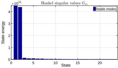
The highest natural frequency of the NREL 5-MW baseline monopile turbine is about 2.5 Hz [11]. Hence, we choose the number of modes for the hydraulic line to be 10, so the line’s modal frequencies are in a wide range of [0, 93.12] Hz. This results in a stable 23rd-order plant Gm. We use the singular perturbation approximation method [12] to reduce the order of

Gmso that the reduced modelGrmcan matchGmwell at low frequencies, which is sufficient for our control design due to slow variations of ωf r. Based on the Hankel singular values of Gm in Fig. 2, we discard 14 states with relatively small singular values. We derive Grm using the Matlab function

0 5 10 _State 15 20

0 1 2 3 4

State energy

×1011 Hankel singular valuesGm

[image:4.612.333.532.52.167.2]

Stable modes

Fig. 2. Hankel singular values of the 23rd-order plantGm.

150 200 250

Magnitude (dB)

10-4 10-2 100 102

0 90 180 270 360

Phase (deg)

Bode Diagram

[image:4.612.337.534.210.318.2]

Frequency (Hz)

Fig. 3. Bode frequency responses of the original 23rd-order plantGmand

its reduced 9th-order modelGrm.

balred[13]. Fig 3 shows the Bode frequency responses of the

original modelGmand the reduced-order modelGrm. Clearly,

GrmmatchesGm very well at frequencies below 40 Hz. Using the H∞ loop-shaping approach [14], we design a

torque controller Km based on Grm to shape the singular values of the open-loop transfer function Gs = GrmKm to match closely those of a desired transfer function Gmd and simultaneously stabilise the closed-loop system. We select

Gmd(s) = 930

(s+ 1e−7)(s+ 50) (3.12)

which has high gain at low frequencies, implying low tracking error in the steady state. Its gain crossover frequency is 17.88 rad/s and the high-frequency roll-off is about -40 dB/decade, which indicates fast tracking performance and good robustness against unstructured model uncertainties. Subsequently, we derive a pre-compensator Wm such that the singular values of GW = GrmWm are identical to those of Gmd in the frequency range [0,∞), using the algorithm proposed by Doyle [15]. The resulting closed loop is unstable because the original (uncompensated) closed-loop system has right-half-plane poles and zeros [16]. To guarantee a stabilising controller, we conductH∞ synthesis [14] by first calculating

a normalised coprime factorisation ofGW:

GW =M_W−1NW (3.13)

in which NWNW∗ +MWMW∗ = 1. The perturbed system of

GW is then written as

˜

0 0.5 1 1.5 2 0

0.2 0.4 0.6 0.8 1 1.2

Time (seconds)

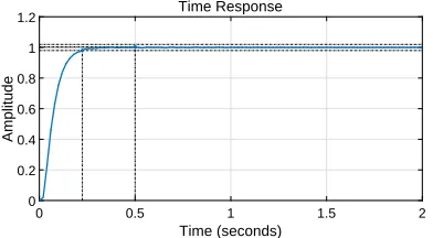
[image:5.612.77.273.57.165.2]

Amplitude

Fig. 4. Closed-loop step response.

where ∆1,∆2 are stable unknown modelling uncertainties.

Now consider finding an optimal H∞ controller Ks to min-imise νs such that

Ks 1

(1−GWKs)−1MW−1

_∞

≤νs. (3.15)

According to Lemma 3.1 in [14],Ksensures the closed-loop stability if

∆1 ∆2

∞≤ν −1

s . Finally, we get the torque controller:

Km=WmKs (3.16)

which can be solved by the Matlab function loopsyn [14]. The resulting closed-loop gain is νs = 1.78, which means that the modelling uncertainties of less than 0.56 are tolerated. The phase and minimum gain margins ofGmKmare 73.4 deg and 11.3 dB, respectively. The closed-loop step response has an overshoot of 0 and a settling time of 0.22 s (see Fig. 4). These results demonstrate that the closed-loop system has good robust stability and tracking performance.

We mention that, since Grm and Gmd are stable and realizable, Wm and GW are stable and realizable [15]. This results in a realizable Ks and thus a realizableKm[14].

B. Pitch Control Using LIDAR Wind Preview

In Region 2, blade pitch control regulates the rotor speed around its rated value. First we design an LPV pitch controller. Then we design an AW compensator for it for the purpose of the system’s recovery after pitch saturation during the transition between Regions 1 and 2. The LPV AW pitch controller uses the steady rotor effective wind speed (estimated by a LIDAR simulator) as the scheduling parameter.

1) LPV Pitch Controller: We design the pitch controller by

taking the rotor/pump shaft dynamics (2.1) and the blade pitch actuator dynamics into account. The latter one is represented by a first-order time delay

˙

β= 1

Tβ

(βd−β) (3.17)

whereβ andβd are the pitch angle and its command, respec-tively.Tβ= 0.1s is the time constant. To maintain the constant rated rotor power in Region 2, the torque controller regulates the pump torque τp to be inversely proportional to the rotor speed ωr. Then (2.1) is rewritten as

˙

ωr= 1

Jr+Jp

τaero(ωr, V, β)−

pr

ωr

(3.18)

wherepr = 5.2966e6W is the rated rotor power. Combining (3.17) and (3.18), we derive a nonlinear model. By linearising it at an operating point (¯ωr,V ,¯ β¯), we obtain

˙ˆ

xp=Apˆxp+Bpβˆd+BpdV ,ˆ ωˆr=Cpˆxp, (3.19)

in which

Ap=

 

fωr+prω2_¯r Jr+Jp

fβ Jr+Jp

0 −1

Tβ

 ,Bp=

h

0 _Tβ1 iT, (3.20)

Cp=1 0,Bpd =

h _fV

Jr+Jp 0

iT

, (3.21)

wherefβ=

∂τaero ∂β

¯

ωr,V ,¯β¯. The state variable vector isxˆp=

ˆ

ωr βˆ

T

, wherexˆp = xp−x¯p in which xp =

ωr β

T

. The input isβˆd=βd−β¯. The disturbance isVˆ =V−V¯. The output is ωˆr =ωr−ω¯r. In Region 2,ω¯r = 12.1rpm. Since the steady values ω¯r and β¯ depend uniquely on V¯ over the entire operating range of the wind turbine, we treat (3.19) as an LPV model withV¯ as the only scheduling parameter.

The design of an LPV pitch controller is to seek a controller

Kp( ¯V) scheduled by V¯ such that for the resulting closed-loop system, the induced L2 norm kF kL2 from the external signalwto the performance outputz=

z1 z2T

satisfies a performance levelγ >0, i.e.,

kF k_L

2= sup w6=0 ¯

V∈Θ

kzk2

kwk₂ < γ (3.22)

in which kxk₂=qR

xT_xdtand

Θ =

  

2

X

j=1

αjθj :αj≥0,

2

X

j=1 αj= 1

  

(3.23)

where θ1 = 11.4m/s and θ2 = 25m/s are the vertices of Θ. Hence, V¯ ∈ Θ means that V¯ varies in Region 2. The control structure is shown in Fig. 5. The external signal w

is the reference value for ωˆr = ωr −ω¯r which is set to be 0 to regulate the rotor speed ωr around its rated value ¯

ωr = 12.1rpm in Region 2. The performance output z is the outputs of weighting functions We and Wu. We select

We = 0._s5₊₅s+0_e−.25₄ , which has high gain at low frequencies to penalise the rotor speed error e and has low gain at high frequencies to limit overshoot. We selectWu= 1.30₀._.1₀₂s+0_s+1.5 to limit control bandwidth and to avoid fast pitch angle variations.

Gp( ¯V) has the state-space realisation (Ap,Bp,Cp,0). Ap (3.20) has the nonlinear termsfωr/(Jr+Jp)andfβ/(Jr+Jp) which depend on V¯ ∈ Θ as shown in Fig. 6. Clearly they can be approximated by two affine functions with V¯ ∈ Θ as the independent variable. Hence, we deemGp( ¯V)affinely dependent on V¯ ∈ Θ. Note that the controller output is

ˆ

βd =βd−β¯whereβ¯is a function ofV¯ (see Fig. 7). Therefore, the actual pitch angle command isβd= ˆβd+ ¯β( ¯V).βˆdis the output of the controllerKp( ¯V)as shown in Fig. 5. We obtain

¯

β( ¯V)by integrating the pitch rateβ˙¯( ¯V) = ˙¯V_dd_Vβ¯¯( ¯V)[17]. Such

     

XA(θj) + ˆBKjC2(θj) + (⋆) ⋆ ⋆ ⋆

ˆ

AT

Kj+A(θj) A(θj)Y+B2(θj) ˆCKj + (⋆) ⋆ ⋆

h

XB1(θj) + ˆBKjD21(θj)

iT

B1(θj)T −γI ⋆

C1(θj) C1(θj)Y+D12(θj) ˆCKj D11(θj) −γI

     

<0 (3.28)

w

_{=0 +}

-e

W

_e

z

₁

ˆ

d

b

_ˆ

r

w

W

_u

z

₂

( )

p

[image:6.612.39.566.52.576.2]

K V

G V

_p

( )

Fig. 5. Control structure of the LPV blade pitch controllerKp( ¯V).

Rotor effective wind speed V (m/s)

10 15 20 25 -3

-2.5 -2 -1.5 -1 -0.5

fβ

/

(

Jr

+

Jp

)

10 15 20 25 -0.8

-0.6 -0.4 -0.2 0

fωr

/

(

Jr

+

Jp

[image:6.612.66.274.268.380.2]

)

Fig. 6. fωr/(Jr+Jp)andfβ/(Jr+Jp)atV¯ ∈Θ.

0 5 10 15 20 25

¯

V(m/s) 0

5 10 15 20 25

¯β

!

¯V

"

(d

eg)

Fig. 7. Steady pitch angleβ¯( ¯V)(V¯is the steady rotor effective wind speed).

induce significant tower loads during the transition between Regions 1 and 2), through limiting dβ/¯ dV¯ to 2.5◦_s/m.

Following the control structure shown in Fig. 5, we obtain an augmented open-loop LPV system PΣ:

˙

x=A( ¯V)x+B1( ¯V)w+B2( ¯V) ˆβd, (3.24)

z=C1( ¯V)x+D11( ¯V)w+D12( ¯V) ˆβd, (3.25)

ˆ

ωr=C2( ¯V)x+D21( ¯V)w. (3.26)

Now we determine a stabilising LPV controller Kp( ¯V) to satisfy (3.22). Recall that Gp( ¯V)depends affinely onV¯ ∈Θ, so does its augmented system PΣ. Hence, according to [18], first we solve an optimisation problem offline: minimising

γX,Y,AˆKj,BˆKj,CˆKj

(j = 1,2) subject to (3.27) and

w=0 +

( ) p

K V bˆd

( )

pa G V

( ) aw

G V

aw

u

aw

y

ˆr

w

d b

Fig. 8. Anti-windup compensation scheme for the LPV pitch controller.

(3.28) with⋆ induced by symmetry.

X I

I Y

>0,X=XT >0,Y=YT >0 (3.27)

Then we derive the controller Kj at the vertex θj with the state-space realisation AKj,BKj,CKj,0in which

AKj =N−p1

ˆ

AKj −XA(θj)Y−BˆKjC2(θj)Y

−XB2(θj) ˆCKj

M−_pT, (3.29)

BKj =N−p1BˆKj,CKj = ˆCKjM−pT, (3.30) where Np and Mp are the solutions of the factorisation problemI−XY=NpMTp. For the online implementation, we measureV¯ and finally obtain the LPV pitch controllerKp( ¯V) with the state-space realisation(AK,BK,CK,0) where

AK BK

CK 0

( ¯V) =

2

X

j=1 αj

AKj BKj

CKj 0

(3.31)

in whichα1= 25₁₃−_.6V¯ andα2 = V¯−₁₃11_.6.4. We mention thatα1

andα2can be any continuous functions ofV¯ satisfying (3.23).

2) AW Compensator: We employ the AW compensation

scheme proposed in [19] for the LPV pitch controller (see Fig. 8). We mention that this AW setup can be incorporated with other pitch controllers because it is designed indepen-dently. This AW scheme is applicable only when the open-loop LPV plant is exponentially stable. However, due to the negative damping introduced by torque control (indicated by the term pr/ω¯2r in (3.20)), the LPV model Gp( ¯V) used for pitch control design is unstable when V¯ is above and near the rated value 11.4 m/s. In order to obtain an exponentially stable LPV plant for the AW design, we neglect this negative damping. Such a treatment (also used in [8], [20]) means that in (3.18) the rotor reaction torquepr/ωris assumed to remain at its constant steady value in Region 2. As a result, the LPV modelGpa( ¯V)used for the AW design is the same asGp( ¯V) withAp in (3.20) replaced with

Apa=

" _f

ωr Jr+Jp

fβ Jr+Jp

0 −_Tβ1

#

[image:6.612.74.273.420.529.2]

As shown in Fig. 8, the AW compensator provides two compensation terms uaw and yaw to the controller out-put and inout-put, respectively. We define the transfer func-tion matrix Gaw( ¯V) of the compensator as Gaw( ¯V) =

M( ¯V)−1 N( ¯V)T

, where N( ¯V) andM( ¯V) are the sta-ble proper coprime transfer functions satisfying Gpa( ¯V) =

N( ¯V)M( ¯V)−1_{. Then its state-space realisation is}

Gaw( ¯V)=s

 

Apa( ¯V) +BpF( ¯V) Bp

F( ¯V) 0

Cp 0



 (3.33)

where F( ¯V) is a state-feedback gain. To ensure quadratic stability of the closed-loop system during saturation and to minimise the effect of yaw on the controller input e, the following condition is required:

M( ¯V)−1

L2<1,

N( ¯V)

L2 < µ, (3.34) which is equivalent to kGawkL2 < µ with µ ≤ 1. To fulfil this condition, we first solve an optimisation problem offline: minimising µ(Q,Hj) (j = 1,2)subject to

   

Apa(θj)Q+BpHj+ (⋆) ⋆ ⋆ ⋆

BT_p −µ ⋆ ⋆

Hj 0 −µ ⋆

CpQ 0 0 −µ

   

<0,

Q=QT >0, µ≤1. (3.35)

Then we obtainF( ¯V)at the vertexθj:F(θj) =HjQ−1. We measure V¯(t)online and the resulting AW compensator is

Gaw( ¯V)=s

2

X

j=1 αj

 

Apa(θj) +BpF(θj) Bp

F(θj) 0

C_p 0



. (3.36)

We use the optimisation tools Sedumi [21] and YALMIP [22] to solve the optimisation problems. Then we derive the LPV pitch controller and its AW compensator. Although they are designed for the case that the scheduling parameter V¯

varies in Region 2, they actually work effectively in the entire operating range of the HWT. When V¯ falls outside Region 2, they choose the state-space data at either the vertex θ1 or

θ2 whichever is closer toV¯. We mention thatV¯ is estimated by a nacelle-based pulsed LIDAR simulator developed by us following Schipf et. al [17].

IV. SIMULATIONSTUDY

In this section we test the performances of our H∞

loop-shaping torque controller and LPV (with/without AW) pitch controller developed in Section III through simulation studies based on the transformed hydrostatic wind turbine (HWT) model developed in Section II. We will compare the perfor-mances of our pitch controller with a gain-scheduled PI pitch controller developed by Laguna [5] (tuned for a simplified NREL 5-MW HWT) whose proportional and integral terms

KP andKI are:

KP(β) =−

1.6167

1 + β

6.302336

, KI(β) =−

0.6929

1 + β

6.302336

. (4.37)

Wind speed (m/s)

50 100 150 200 250 300 Time (seconds)

10 15 20

50 100 150 200 250 300 8

[image:7.612.331.537.53.163.2] [image:7.612.323.537.223.329.2]

10 12 14 16 18

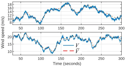
Fig. 9. Actual and estimated (by LIDAR) rotor effective wind speeds (V

andV¯) under the turbulent wind input with a mean speed of 11.4 m/s (top) or 18 m/s (bottom) along with a wave input.

Pressure difference

across the pump (bar)

50 100 150 200 250 300 Time (seconds)

250 300

350 50 100 150 200 250 300 200

250 300 350

Fig. 10. Pressure commandPpdand actual pressure difference across the

pumpPpunder the turbulent wind input with a mean speed of 11.4 m/s (top)

or 18 m/s (bottom) along with a wave input.

We also design a back-calculation AW compensator [23] for the above PI controller. The back-calculation coefficient is tuned to be 0.5.

[image:7.612.64.298.312.377.2]

We use two IEC full-field turbulent wind inputs together with a same irregular wave input during the simulations. The wind inputs are generated by NREL TurbSim [24] using the Class I Extreme Turbulence Model (ETM) with mean speeds of 11.4 m/s (rated speed) and 18 m/s, respectively. The waves are irregularly generated based on the JONSWAP/Pierson-Moskowitz spectrum by the HydroDyn module of FAST. The peak-spectral period and significant wave height of the incident waves are 10 seconds and 6 m, respectively.

Fig. 9 shows the actual rotor effective wind speedV (com-puted by FAST AeroDyn) and its estimationV¯ (by LIDAR). Clearly, the correlation between these two signals at low frequencies is good. This is very desirable since the low-frequency components contain the most wind power and affect the turbine most [25]. Besides, under either wind input, V

covers both Regions 1 and 2 as shown in Fig. 9. Fig. 10 shows that ourH∞loop-shaping torque controller tracks the pressure

command Ppd (3.10) effectively. The LPV AW controller is used for pitch control here.

Tables I and II list the performances of 4 different pitch controllers under the two wind inputs respectively, along with the same wave input. The same H∞ loop-shaping torque

TABLE I

PERFORMANCES OF4PITCH CONTROLLERS UNDER THE TURBULENT WIND INPUT WITH A MEAN SPEED OF11.4M/S ALONG WITH A WAVE INPUT. CHANGES W.R.T.THEPICASE ARE GIVEN IN THE BRACKETS.

PI LPV LPV AW PI AW Average

power (kW) 4309.8

4398.0 (2.05%)

4373.0 (1.47%)

4331.8 (0.51%) Standard deviation

of power (kW) 750.34

697.93 (-6.98%)

695.45 (-7.32%)

724.94 (-3.39%) Standard deviation

of pitch rate (deg) 1.20

0.61 (-49.17%)

0.74 (-38.33%)

0.88 (-26.67%) Fore-aft

DEQL (kN·m) 20614

7854.0 (-59.11%)

6197.7 (-69.93%)

7772.6 (-62.29%)

Side-to-side

DEQL (kN·m) 5941.1

2338.2 (-60.64%)

2064.4 (-65.25%)

2836.3 (-52.26%)

TABLE II

PERFORMANCES OF4PITCH CONTROLLERS UNDER THE TURBULENT WIND INPUT WITH A MEAN SPEED OF18M/S ALONG WITH A WAVE INPUT.

CHANGES W.R.T.THEPICASE ARE GIVEN IN THE BRACKETS.

PI LPV LPV AW PI AW Average

power (kW) 4625.0

4681.1 (1.21%)

4679.8 (1.18%)

4628.1 (0.067%) Standard deviation

of power (kW) 393.73

288.33 (-26.77%)

287.38 (-27.01%)

369.79 (-6.08%) Standard deviation

of pitch rate (deg) 1.11

0.79 (-28.83%)

0.81 (-27.03%)

0.99 (-10.81%) Fore-aft

DEQL (kN·m) 15872

8074.8 (-49.13%)

8007.1 (-49.55%)

9392.0 (-40.83%) Side-to-side

DEQL (kN·m) 5764.0

4336.1 (-24.77%)

4173.7 (-27.59%)

5748.7 (-0.27%)

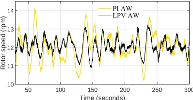
the monopile base using the NREL MLife code [27] based on the time-series of the monopile base fore-aft and side-to-side moments. As indicated in Tables I & II, our PI AW controller and LPV controllers (with and without AW) attain much better overall performances than the PI controller developed by Laguna [5] under either wind input along with the wave input, including increased average power, improved regulation of the rotor speed & generator power, and considerably reduced damage on the blade bearings & monopile tower. Considering the two cases with AW, the LPV AW controller is superior to the PI AW one especially in terms of mitigating the loads on the blade bearings & monopile tower. Fig. 11 shows the simulation results for the cases using three types of pitch controllers under the turbulent wind input with a mean speed of 11.4 m/s along with the wave input, which further verifies the conclusions from Table I. In addition, it is noticeable from Fig. 11 that significant rotor speed, generator power and tower loading variations occur due to pitch saturation during the transitions at about 55 s and 110 s (see the top diagram of Fig. 9) for the cases using the PI and LPV (without AW) controllers, while the LPV AW pitch controller achieves much smoother responses. We mention that similar phenomena are found under the turbulent wind input with a mean speed of 18 m/s along with the wave input. To avoid overlap, we only give the plot of the rotor speed responses for the cases using

50 100 150 200 250 300

10 12 14 16 18

Rotor speed (rpm)

(a)

50 100 150 200 250 300

0 5 10 15 20

Collective blade pitch angle (deg)

(b)

50 100 150 200 250 300

2500 3000 3500 4000 4500 5000

Generator power (kW)

(c)

50 100 150 200 250 300

-1.5 -1 -0.5 0 0.5 1

Monopile base

fore-aft moment (kN

·

m

)

×105

(d)

50 100 150 200 250 300

Time (seconds)

-1 -0.5 0 0.5 1 1.5 2

Monopile base

side-to-side moment (kN

·

m

) × 104

(e)

50 100 150 200 250 300 Time (seconds)

10 11 12 13 14

[image:9.612.73.272.60.163.2]

Rotor speed (rpm)

Fig. 12. Rotor speed responses under the turbulent wind input with a mean speed of 18 m/s along with a wave input.

the PI AW and LPV AW controllers in Fig. 12 where the LPV AW controller regulates the rotor speed much more tightly than its PI AW counterpart.

V. CONCLUSIONS

We transformed the NREL 5-MW geared equipped monopile wind turbine model within FAST into a detailed aero-hydro-servo-elastic hydrostatic wind turbine simulation model. We then designed an H∞ loop-shaping torque

con-troller and a LIDAR-based LPV AW pitch concon-troller. The simulation results showed good tracking behaviours achieved by our torque controller and much improved overall perfor-mances attained by our LPV (with or without AW) pitch control scheme compared with a gain-scheduled PI pitch control system developed by Laguna [5], in terms of rotor speed regulation, power quality, and load reductions of the blade bearings & monopile tower.

One of the future directions is to develop a more detailed HST drivetrain system which incorporates the dynamics of auxiliary hydraulic components (e.g., the charging system, pressure relief valves, accumulators, and flow control valves).

REFERENCES

[1] J.-C. Ossyra, “Reliable, lightweight transmissions for off-shore, utility scale wind turbines,” Eaton Corporation, WI, USA, Tech. Rep., 2012. [2] R. Dutta, “Modeling and analysis of short term energy storage for

mid-size hydrostatic wind turbine,” Master’s thesis, Uni. of Minnesota, 2012. [3] F. Wang and K. A. Stelson, “Model predictive control for power optimization in a hydrostatic wind turbine,” in 13th Scandinavian International Conference on Fluid Power, Sweden, Jun 2013. [4] B. Skaare, B. H¨ornsten, and F. G. Nielsen, “Modeling, simulation and

control of a wind turbine with a hydraulic transmission system,”Wind Energy, vol. 16, no. 8, pp. 1259–1276, 2013.

[5] A. J. Laguna, “Modeling and analysis of an offshore wind turbine with fluid power transmission for centralized electricity generation,”Journal of Computational and Nonlinear Dynamics, vol. 10, p. 041002, 2015. [6] A. J. Laguna, N. F. Diepeveen, and J. W. Van Wingerden, “Analysis of

dynamics of fluid power drive-trains for variable speed wind turbines: parameter study,”IET Renewable Power Generation, vol. 8, no. 4, pp. 398–410, 2014.

[7] X. Tong, X. Zhao, and S. Zhao, “Load reduction of a monopile wind turbine tower using optimal tuned mass dampers,”International Journal of Control, vol. 90, no. 7, pp. 1283–1298, 2017.

[8] J. Jonkman, S. Butterfield, W. Musial, and G. Scott, “Definition of a 5-MW reference wind turbine for offshore system development,” National Renewable Energy Laboratory (NREL), CO, USA, Tech. Rep., 2009. [9] J. M. Jonkman and M. L. Buhl Jr, “FAST users guide,” National

Renewable Energy Laboratory (NREL), CO, USA, Tech. Rep., 2005. [10] J. Makinen, R. Piche, and A. Ellman, “Fluid transmission line modeling

using a variational method,”Journal of dynamic systems, measurement, and control, vol. 122, no. 1, pp. 153–162, 2000.

[11] P. Passon, M. K¨uhn, S. Butterfield, J. Jonkman, T. Camp, and T. J. Larsen, “OC3—benchmark exercise of aero-elastic offshore wind turbine codes,” in EAWE Special Topic Conference: The Science of Making Torque from Wind, Lyngby, Denmark, Aug. 2007.

[12] Y. Liu and B. D. Anderson, “Singular perturbation approximation of balanced systems,”International Journal of Control, vol. 50, no. 4, pp. 1379–1405, 1989.

[13] A. Varga, “Balancing free square-root algorithm for computing singular perturbation approximations,” in30th IEEE Conference on Decision and Control, Brighton, UK, December 1991.

[14] K. Glover and D. McFarlane, “Robust stabilization of normalized coprime factor plant descriptions withH∞-bounded uncertainty,”IEEE

Transactions on Automatic Control, vol. 34, no. 8, pp. 821–830, 1989. [15] J. Doyle, “Advances in multivariable control,” Lecture Notes at

ONR/Honeywell Workshop, MN, USA, October 1984.

[16] D. McFarlane and K. Glover, “A loop-shaping design procedure using

H∞synthesis,”IEEE Transactions on Automatic Control, vol. 37, no. 6,

pp. 759–769, 1992.

[17] D. Schipf, E. Simley, F. Lemmer, L. Y. Pao, and P. W. Cheng, “Collective pitch feedforward control of floating wind turbines using lidar,”Journal of Ocean and Wind Energy, vol. 2, no. 4, pp. 223–230, 2015. [18] P. Apkarian and R. J. Adams, “Advanced gain-scheduling techniques for

uncertain systems,”IEEE Transactions on control systems technology, vol. 6, no. 1, pp. 21–32, 1998.

[19] M. C. Turner and I. Postlethwaite, “A new perspective on static and low order anti-windup synthesis,”International Journal of Control, vol. 77, no. 1, pp. 27–44, 2004.

[20] M. H. Hansen, A. D. Hansen, T. J. Larsen, S. Øye, P. Sørensen, and P. Fuglsang, “Control design for a pitch-regulated, variable speed wind turbine,” Risø National Laboratory, Denmark, Tech. Rep., 2005. [21] J. F. Sturm, “Using SeDuMi 1.02, a MATLAB toolbox for optimization

over symmetric cones,”Optimization methods and software, vol. 11, no. 1-4, pp. 625–653, 1999.

[22] J. Lofberg, “YALMIP: A toolbox for modeling and optimization in MATLAB,” in13th IEEE International Symposium on Computer Aided Control System Design, Taipei, Taiwan, September 2004, pp. 284–289. [23] A. Izadbakhsh, A. A. Kalat, M. M. Fateh, and M. R. Rafiei, “A robust anti-windup control design for electrically driven robots—theory and experiment,”International Journal of Control, Automation and Systems, vol. 9, no. 5, pp. 1005–1012, 2011.

[24] B. J. Jonkman, “TurbSim user’s guide: Version 1.50,” National Renew-able Energy Laboratory (NREL), CO, USA, Tech. Rep., 2009. [25] F. Dunne, L. Y. Pao, D. Schlipf, and A. K. Scholbrock, “Importance of

lidar measurement timing accuracy for wind turbine control,” in 2014 American Control Conference, OR, USA, Jun 2014, pp. 3716–3721. [26] K. Z. Østergaard, J. Stoustrup, and P. Brath, “Linear parameter varying

control of wind turbines covering both partial load and full load conditions,” International Journal of Robust and Nonlinear Control, vol. 19, no. 1, pp. 92–116, 2009.