warwick.ac.uk/lib-publications
Original citation:Price, Leah F., Drovandi, Christopher C., Lee, Anthony and Nott, David J. (2017) Bayesian synthetic likelihood. Journal of Computational and Graphical Statistics.
Permanent WRAP URL:
http://wrap.warwick.ac.uk/85427
Copyright and reuse:
The Warwick Research Archive Portal (WRAP) makes this work by researchers of the University of Warwick available open access under the following conditions. Copyright © and all moral rights to the version of the paper presented here belong to the individual author(s) and/or other copyright owners. To the extent reasonable and practicable the material made available in WRAP has been checked for eligibility before being made available.
Copies of full items can be used for personal research or study, educational, or not-for profit purposes without prior permission or charge. Provided that the authors, title and full bibliographic details are credited, a hyperlink and/or URL is given for the original metadata page and the content is not changed in any way.
Publisher’s statement:
“This is an Accepted Manuscript of an article published by Taylor & Francis. Journal of Computational and Graphical Statistics con 06/03/2017 available online:
http://dx.doi.org/10.1080/10618600.2017.1302882
A note on versions:
The version presented here may differ from the published version or, version of record, if you wish to cite this item you are advised to consult the publisher’s version. Please see the ‘permanent WRAP URL’ above for details on accessing the published version and note that access may require a subscription.
Bayesian Synthetic Likelihood
L. F. Price and C. C. Drovandi
∗School of Mathematical Sciences, Queensland University of Technology, Australia
Australian Research Council Centre of Excellence for
Mathematical and Statistical Frontiers (ACEMS)
A. Lee
Department of Statistics, University of Warwick, UK
D. J. Nott
†Department of Statistics and Applied Probability, National University of Singapore
January 18, 2017
Abstract
Having the ability to work with complex models can be highly beneficial. How-ever, complex models often have intractable likelihoods, so methods that involve evaluation of the likelihood function are infeasible. In these situations, the benefits of working with likelihood-free methods become apparent. Likelihood-free methods, such as parametric Bayesian indirect likelihood that uses the likelihood of an alter-native parametric auxiliary model, have been explored throughout the literature as a viable alternative when the model of interest is complex. One of these methods is called the synthetic likelihood (SL), which uses a multivariate normal approximation of the distribution of a set of summary statistics. This paper explores the accuracy and computational efficiency of the Bayesian version of the synthetic likelihood (BSL) approach in comparison to a competitor known as approximate Bayesian computation (ABC) and its sensitivity to its tuning parameters and assumptions. We relate BSL to pseudo-marginal methods and propose to use an alternative SL that uses an un-biased estimator of the SL, when the summary statistics have a multivariate normal distribution. Several applications of varying complexity are considered to illustrate the findings of this paper. Supplemental materials are available online.
∗LFP and CCD are grateful to Mat Simpson for assistance with the cell biology example. CCD thanks
NUS and the University of Warwick for supporting a visit where discussions on this research took place. LFP was supported by an Australian Postgraduate Award. CCD was supported by an Australian Research Council’s Discovery Early Career Researcher Award funding scheme DE160100741.
†DJN was supported by a Singapore Ministry of Education Academic Research Fund Tier 2 grant
1
Introduction
Statisticians and applied practitioners often desire the ability to work with complex
sta-tistical models. Such models can lead to a more complete understanding of the process
believed to generate the observed data, in comparison to simpler models that are easy to
fit computationally. One computational issue with complex models is that the likelihood
function can be very difficult or impossible to compute, precluding the use of standard,
likelihood-based approaches to inference. In such settings, likelihood-free methods
facili-tate inference by approximating the likelihood function in particular ways.
There are some likelihood-free methods that work on the full data level, but it is
com-mon practice to reduce the data to a summary statistic for computational or practical
pur-poses (see Blum et al. (2013) for an outline of data reduction techniques). When summary
statistics are used, a range of likelihood-free methods including approximate Bayesian
com-putation (ABC, see Sisson and Fan (2011) for example) and the synthetic likelihood (SL)
method of Wood (2010), which uses a multivariate normal approximation of the
distribu-tion of a set of summary statistics, are applicable. Even though Wood (2010) incorporates
the SL within a Markov chain Monte Carlo (MCMC) algorithm, the focus of Wood (2010)
is to determine the maximum SL estimator, i.e. a classical approach. It is trivial to consider
a Bayesian version of this, by assigning a prior distribution on the parameter. Then the
output of the MCMC algorithm of Wood (2010) would be a sample from an approximated
probability distribution of the parameter conditional on the observed summary statistic.
We refer to this approach as Bayesian synthetic likelihood (BSL), which is the focus of this
paper.
In contrast, ABC uses a non-parametric auxiliary likelihood as a replacement to the
intractable likelihood (Blum, 2010; Drovandi et al., 2015) and is currently regarded as
the state-of-the-art method of approximation when data have been reduced to a summary
statistic. Assume that there is interest in the parameter θ ∈ Θ of a stochastic process
and the observed data y ∈ Y has been generated from this model. In ABC, data x is
simulated from the model based on a proposedθ and the observed, sy ∈S, and simulated,
sx ∈ S, summary statistics are compared. Denote n independent simulated datasets as
statistic associated with xi is denoted si for notational convenience. ABC estimates the
intractable summary statistic likelihood, p(sy|θ), non-parametrically:
p,n(sy|θ) =
1
n
n X
i=1
K(ρ(sy,si)), (1)
whereρ(sy,sx) measures the distance between the observed and simulated summary
statis-tics andK(·) is a kernel weighting function with bandwidth(known as the ABC tolerance)
designed to give larger weight to smaller ρ. Despite the extensive research performed on
ABC, there still remains no standard way to select these tuning parameters. ABC can be
viewed as a pseudo-marginal method (Andrieu and Roberts, 2009), since p,n(sy|θ) in (1)
is an unbiased estimate of the ABC likelihood, p(sy|θ), which is given by
p(sy|θ) =
Z
Y
p(x|θ)K(ρ(sy,sx))dx.
Using the theory of Andrieu and Roberts (2009), the ABC target is not influenced by the
choice of nwhen the ABC likelihood (1) is incorporated in an MCMC algorithm. However,
ABC is known to be highly sensitive to the choice of , the discrepancy function and to a
lesser extent the kernel weighting function (Marin et al., 2012).
Since BSL by definition uses a multivariate normal approximation, it depends only on
a single tuning parameter, n, which is the number of replicated simulations of the model
used in estimating the mean and covariance matrix of the multivariate normal auxiliary
model, denoted by µn and Σn respectively. BSL uses the following estimate
pA,n(sy|θ) =N(sy;µn(θ),Σn(θ)), (2)
in place of the intractable likelihood of the summary statistic. The BSL target depends on
n as N(sy;µn(θ),Σn(θ)) is not an unbiased estimate of N(sy;µ(θ),Σ(θ)). Due to this
dependence on n, there is interest in investigating the sensitivity of BSL to this tuning
parameter. The subscriptA denotes that the target also depends on the choice of auxiliary
model, which in the case of BSL is multivariate normal. Alternative parametric auxiliary
models can be considered as part of a wider framework referred to as parametric Bayesian
indirect likelihood on the summary statistic level (psBIL) by Drovandi et al. (2015). This
general framework is described in Appendix A of the supplementary materials, though the
The main aim of this article is to explore the use of the SL within a Bayesian framework.
This involves exploring the sensitivity of BSL to its tuning parameter n, the multivariate
normal assumption and assessing the computational efficiency of the approach. We find
empirically that the target distribution provided by BSL is remarkably insensitive to n.
Due to this we are able to choose n to maximise computational efficiency and consider
guidance from the literature on pseudo-marginal methods (Andrieu and Roberts, 2009).
Furthermore, we propose to use an estimator of the normal likelihood that is exactly
un-biased when the summary statistics are multivariate normal, based on a density estimator
due to Ghurye and Olkin (1969). Using this exactly unbiased estimator creates a novel
pseudo-marginal BSL method that is theoretically unaffected by n under the multivariate
normality assumption for the summary statistic. In a toy application we show that BSL
becomes increasingly more computationally efficient than ABC as the dimension of the
summary statistic rises beyond 2. BSL also seems to be more efficient than ABC as the
dimension of the summary statistic is increased in more realistic examples. Finally, we
consider scenarios where BSL does not perform well.
Since its inception, the SL has shown promising results in substantive applications (see,
for example, Brown et al. (2014)). The SL has also been considered within a Bayesian
framework. Hartig et al. (2014) apply BSL to the FORMIND forest model. Fasiolo et al.
(2016) employ BSL and compare it with particle MCMC (Andrieu et al., 2010) for
applica-tions in ecology and epidemiology (see also Fasiolo and Wood (2016)). Everitt et al. (2016)
use BSL for models that have an intractable normalising constant. Meeds and Welling
(2014), Wilkinson (2014), Moores et al. (2015) and Gutmann and Corander (2015) use
em-ulation to speed up the calcem-ulations involved in BSL. Meeds and Welling (2014) consider
Gaussian process surrogate modelling of each marginal summary statistic, ignoring
poten-tial correlation between summaries. Wilkinson (2014) consider Gaussian process surrogate
modelling of the log SL. Gutmann and Corander (2015) develop a similar approach to
Wilkinson (2014) but use Bayesian optimisation (e.g. Jones (2001)) to train the GP rather
than the sequential history matching approach (e.g. Craig et al. (1997)) used in Wilkinson
(2014). Moores et al. (2015) use non-parametric modelling of the relationship between the
Despite this research, no attention has been given to how the value ofn affects BSL and no
comparison to its natural competitor, ABC. Furthermore, as mentioned earlier, we create
a new BSL method.
In Section 2 of this paper, the BSL method is described in further detail, including an
outline of the notation used throughout this paper. Section 3 compares the computational
efficiency of ABC and BSL on a toy example. The empirical results are provided in Section
4 on models and datasets with varying complexity. A discussion is provided in Section 5,
which also points to further research directions.
2
Bayesian Synthetic Likelihood
2.1
Framework
In a Bayesian framework, the objective is to determine an approximation to the posterior
distribution p(θ|y) ∝ p(y|θ)p(θ) where y ∈ Y is data of dimension N coming from the
assumed stochastic model. The model is considered to be so complex that the likelihood
function,p(y|θ), is not computationally tractable. In the SL method and in psBIL methods
more generally, a summary statistic of this data, sy ∈ S ⊆ Rd where d is the number of
statistics, is all that is required. The posterior distribution and likelihood become p(θ|sy)
and p(sy|θ), respectively. If sy carries most of the information contained in the observed
data, y, then p(θ|sy) can be close to p(θ|y). We note also that the aim is not always
to target the full posterior as discarding some information can be useful to improve the
behaviour of the likelihood, for example in the near-chaotic systems of Wood (2010), or to
make the inference more robust to model misspecifications. Since the full data likelihood is
intractable, it is likely thatp(sy|θ) is also intractable. In Appendix A of the supplementary
materials, a general framework for applying parametric approximations of this intractable
likelihood is given.
Due to its suitability under many circumstances and its computational convenience,
Wood (2010) use an auxiliary likelihood based on a multivariate normal approximation,
referred to as the synthetic likelihood. Here we have auxiliary parameters µ(θ) andΣ(θ),
covariance matrix of the multivariate normal distribution. In generalµandΣare unknown
but can be estimated by simulating n iid data sets of size N from the model based on θ
and fitting the auxiliary likelihood to the summary statistics,s1:n. The estimated auxiliary likelihood is N(sy;µn(θ),Σn(θ)), with the following analytic expression for the auxiliary
parameter estimates
µn(θ) = 1
n
n X
i=1
si, Σn(θ) = 1
n−1 n X
i=1
(si−µn(θ))(si−µn(θ))>. (3)
BSL arises when this auxiliary likelihood is combined with a prior distribution on the
parameter. Following Drovandi et al. (2015), BSL samples from the following target
pA,n(θ|sy)∝pA,n(sy|θ)p(θ), (4)
where
pA,n(sy|θ) =
Z
Sn
N(sy;µn(θ),Σn(θ))
n Y
i=1
p(si|θ)ds1:n. (5)
By taking a single draw of s1:n
iid
∼ p(·|θ) and computing N(sy;µn(θ),Σn(θ)) we obtain
an unbiased estimate of pA,n(sy|θ). Under the mild condition that (4) is integrable as a
function of θ, using the stochastic and non-negative estimator N(sy;µn(θ),Σn(θ)) in an
MCMC algorithm (see later) produces a pseudo-marginal algorithm (Andrieu and Roberts,
2009) that targets (4). It is important to note that pA,n(θ|sy) is not equal to the ‘ideal’
BSL target, pA(θ|sy) ∝ N(sy;µ(θ),Σ(θ))p(θ). Nevertheless, Drovandi et al. (2015) do
show under mild conditions that the ideal BSL target will be achieved as n → ∞. Later in
this section, we develop an alternative BSL method that does target pA(θ|sy), under the
assumption that the summary statistic is indeed multivariate normal.
As demonstrated above, the target distribution of BSL depends on the multivariate
normal approximation and on the selection of n (since pA(sy|µn(θ),Σn(θ)) is not an
un-biased estimator of pA(sy|µ(θ),Σ(θ))). There is interest, then, on the sensitivity of BSL
to the choice of n and its robustness towards departures from normality of the summary
statistic, which we investigate empirically in Section 4. We use an MCMC algorithm with
T iterations to sample frompA,n(θ|sy), which is shown in Appendix B of the supplementary
iteration, a simulation step in order to obtain µn(θ) and Σn(θ) of the SL. Wood (2010)
adopts the same approach but uses the output to maximise the SL, rather than using the
samples to construct a posterior distribution. We refer to this algorithm as MCMC BSL.
Under the assumption that the summary statistic is normally distributed and the
ob-served summary statistic sy is fixed, we point out that there is an exactly unbiased,
non-negative estimator of a normal density function due to Ghurye and Olkin (1969,§3.4), and
which results in a valid pseudo-marginal algorithm targeting pA(θ|sy) for any n > d+ 3
rather than pA,n(θ|sy), which is only an approximation of pA(θ|sy). We refer to the
unbi-ased estimator of the SL as uSL and the resulting Bayesian procedure as uBSL, where ‘u’
denotes unbiased. Using the notation of Ghurye and Olkin (1969), let
c(k, v) = 2
−kv/2π−k(k−1)/4
Qk i=1Γ
1
2(v−i+ 1)
,
and for a square matrix Awrite ψ(A) =|A|if A>0 and ψ(A) = 0 otherwise, where |A|
is the determinant ofAandA>0 means thatAis positive definite. The result of Ghurye
and Olkin (1969) shows that an exactly unbiased estimator of N(sy;µ(θ),Σ(θ)) is (in the
case where the summary statistics are normal and n > d+ 3)
ˆ
pA(sy|θ) = (2π)−d/2
c(d, n−2)
c(d, n−1)(1−1/n)d/2|Mn(θ)|
−(n−d−2)/2
ψ Mn(θ)−(sy−µn(θ))(sy−µn(θ))>/(1−1/n)
(n−d−3)/2
,
whereMn(θ) = (n−1)Σn(θ). The estimated likelihood, ˆpA(sy|θ), replacesN(sy;µn(θ),Σn(θ))
in MCMC BSL to create the novel MCMC uBSL algorithm. We stress that this algorithm
targetspA(θ|sy) (notp(θ|sy)) under the multivariate normality assumption of the summary
statistic, which can be made approximately valid through appropriate choice or
transfor-mation of the summary statistic (Wood, 2010). The appeal of this approach is that the
approximate posterior it induces may have less dependence on ncompared to the standard
implementation of MCMC BSL. We discuss this further in the next section and investigate
it empirically in Section 4.
2.2
Choice of
n
MCMC BSL is similar to the grouped independence Metropolis-Hastings (GIMH) algorithm
the likelihood estimate for the current θ is carried over to the next iteration (it is not
re-estimated). Specifically, the GIMH algorithm is a pseudo-marginal method (Andrieu and
Roberts, 2009) where a non-negative and unbiased likelihood estimator is used in place of
the intractable likelihood. Andrieu and Roberts (2009) show that the GIMH method has
as its limiting distribution the desired posterior distribution. In our case, the auxiliary
likelihood estimator based on n is not an unbiased estimator of the auxiliary likelihood
obtained if it were possible to take n → ∞, despite using unbiased estimators of the
mean vector, µ(θ), and covariance matrix, Σ(θ). However, we demonstrate with strong
empirical evidence in Section 4 that under the assumptions that the distribution of the
summary statistic is not highly irregular and the model is able to recover sy, the BSL
target shows little sensitivity ton. Therefore we conjecture that, under these assumptions,
the bias in the SL estimator decreases fairly rapidly so that small to moderatenis sufficient.
Given the apparent insensitivity of the BSL posterior to n, we suggest to choose n in
order to maximise the overall computational efficiency. A small value of n reduces the
computation time per iteration, but will result in highly variable estimates of the SL. It
is well known that the GIMH algorithm can become stuck if the likelihood for some θ is
grossly overestimated. On the other hand, ifnis set large, the SL is estimated precisely, but
the computation time per iteration is high. Borrowing the theoretical result for the GIMH
method outlined in Doucet et al. (2015), the value of n should be chosen such that the
log SL at some θ with high (BSL) posterior support should be estimated with a standard
deviation of roughly 1. We investigate this recommendation in Section 4.
The MCMC uBSL target is theoretically unaffected byn if the multivariate normality
assumption of the summary statistic holds. However, given that this assumption is unlikely
to hold in practice, the sensitivity of MCMC uBSL to the value of n is of interest, which
we explore empirically in Section 4. It is important to note that the random variable
describing the uSL is a mixture of a discrete and a continuous random variable; it may
be identically 0 if the argument of ψ(·) is not positive definite, implying that the log uSL
is −∞ in such cases. Hence the standard deviation of the log uSL is infinite generally,
meaning that we cannot consider the guidance of Doucet et al. (2015) for pseudo-marginal
In Section 3 we demonstrate on a toy example that BSL becomes increasingly more
computationally efficient relative to ABC with an increase in the dimension of the
sum-mary statistic. This is an expected result as BSL uses a parametric approximation to the
summary statistic likelihood as opposed to the non-parametric one used in ABC. However,
we find empirically in Section 4 that for BSL the optimal n in terms of computational
efficiency increases with the dimension of the summary statistic. Thus BSL is unable to
completely escape the curse of dimensionality issue. Therefore, as in the case of ABC, the
choice of summary statistic in BSL is important to keep the computation to a manageable
level.
2.3
Normality Assumption
In many applications the central limit theorem may justify the use of the multivariate
normal approximation of the distribution of the summary statistic (Wood, 2010). In cases
where the normality assumption does not hold, Wood (2010) suggests to apply an
appro-priate transformation. However, in complex problems with a high dimensional summary
statistic, it may not be feasible to investigate such transformations in great detail. Hence,
of interest is the robustness of the BSL method to departures from normality.
A possible on-line diagnostic tool for BSL would involve performing a hypothesis test for
multivariate normality (or at least a test for normality on each component of the summary
statistic) at every iteration of MCMC BSL. Unfortunately, to achieve sufficient power in
these tests a large value of n is required, which is not computationally efficient. This is
consistent with Wood (2010) in the context of SL. Despite this, we adopt this approach to
investigate the robustness of BSL when there is evidence against the normality assumption.
3
Efficiency Comparison to ABC
ABC approximates the intractable summary statistic likelihood,p(sy|θ), with the following
approximate likelihood
p(sy|θ) = Z
Y
A common choice for the kernel weighting functionK(·) is the indicator functionK(ρ(sy,sx))∝
I(ρ(sy,sx) ≤ ) while in this paper we consider the Gaussian kernel, K(ρ(sy,sx)) ∝
exp
−ρ(sy2,sx)2. The integral to compute the ABC likelihood in (6) is analytically in-tractable but it can be unbiasedly estimated by simulation, which is sufficient to generate
an MCMC kernel that targets p(θ|sy)∝p(sy|θ)p(θ) (Andrieu and Roberts, 2009). The
estimated ABC likelihood is given in (1). The results of Bornn et al. (2016) suggest that,
in a serial computing environment, n = 1 is close to optimal. Below we compare the
computational efficiency of ABC and BSL on a toy example.
It is well known that ABC suffers a curse of dimensionality with respect to the size of
the summary statistic (Blum et al., 2013). The multivariate normality assumption in BSL
may deteriorate with the size of the summary statistic, so that BSL still suffers from a curse
of dimensionality but in a different manner. However, intuitively one might expect BSL
to be more computationally efficient than ABC due to the use of a parametric auxiliary
model. The following toy example provides some insight. We will assume the unknown
likelihood isp(y|θ) = N(y;θ,Σ) whereΣis some fixed and known covariance matrix. The
auxiliary model is pA(y|φ) = N(y;φ,Σ), and one is interested in knowing which of the
two methods (standard ABC vs BSL) is more effective. Such a comparison is aided by the
fact that there is a correspondence between pA,n(y|θ) and p(y|θ) in this particular case,
with K(x,y) = N(y;x, Σ) and φn(θ) = n−1Pni=1xi. Indeed, elementary calculations provide that when =n−1, pA,n(y|θ) =N(y;θ,Σ(1 +)) =p(y|θ).
Since the two different auxiliary models define the same approximate likelihood, they
induce the same posterior distribution for a given prior distribution. The main difference
is how the likelihood N(y;θ,Σ(1 +)) is estimated within a Monte Carlo method. In
ABC, the approximation is Z1(θ) = N(y;x1, Σ), x1 ∼ N(·;θ,Σ), whereas in BSL the
approximation is Z2(θ) =N(y;x2,Σ),x2 ∼ N(·;θ, n−1Σ).
The full details on the efficiency comparison for this toy example can be found in
Appendix C of the supplementary materials. Here we provide the main results. In a
rejection sampling framework, we find that the ratio of the ABC acceptance rate against
the BSL acceptance rate is d/2. ABC requires on average nd/2 more samples of x1 than
random variables, and recalling that = n−1 we obtain that an ABC rejection sampler is more computationally efficient when d = 1, equally computationally efficient when d = 2
and becomes significantly less efficient as d increases beyond 2.
For other Monte Carlo methods, it is of some interest to consider the relative variance
of the estimates Z1(θ) and Z2(θ). We find that var (Z2(θ))<var (Z1(θ)) for any (y,θ,Σ),
∈ (0,1), and d≥ 1. The relative variance of Z2(θ) converges to 0 as → 0. In fact, we
have that the relative variance of Z1(θ) is in O(−d/2) as →0. It follows that if we define
Z1,M(θ) to be an average ofM iid replicates ofZ1(θ) then one would need to increaseM at
least by nd/2 in order to control the relative variance. Once again, by taking into account
the fact that simulatingZ2(θ) involves averagingn N(θ,Σ) random variables, this implies
that as d increases beyond 2 BSL becomes significantly more computationally efficient.
Since the above result is limited to the toy application considered and that BSL
es-timates Σ(θ) rather than using a fixed Σ, we attempt to compare the computational
efficiency of BSL and ABC on the examples in the next section.
4
Examples
Here results for BSL and uBSL are obtained for several simulation studies. These involve
investigating the sensitivity of the BSL approaches to n, robustness against the normality
assumption and comparisons to ABC in terms of computational efficiency. We note that
it is generally difficult to fairly compare the efficiency of different methods, especially
when they result in different target densities. In addition, ABC has a number of tuning
parameters, which further complicates the comparison. For some of the examples the
targets produced are similar so in these cases we use the same proposal distribution in the
BSL and ABC MCMC algorithms. To simplify the comparisons we use efficient starting
values and proposal distributions that are informed by pilot runs as described in Appendix
D of the supplementary materials. We assume that model simulation consumes the majority
of computing time in the simulation-based methods we consider in this paper. Thus to
compare efficiency, we compute the effective sample size (ESS) for each parameter obtained
from the CODA package in R (Plummer et al., 2006) and standardise it by the number
increase the magnitude to facilitate easy comparison. We refer to this as the normalised
ESS value.
We attempt to give an advantage to the ABC approach by assigning what might be
considered an efficient discrepancy function. Using the true parameter value, which is
obviously unavailable in practice, a number of simulations are generated from the model
and the summary statistics calculated. Then the sample covariance matrix of the summary
statistic is computed and subsequently used in a Mahalanobis discrepancy function for
ABC. Devising an efficient discrepancy function in ABC is a non-trivial task and may
involve some pilot runs. BSL avoids this extra tuning and computation. A Gaussian
function with variance is used as the kernel weighting function. We choose the value
for ABC so that it produces similar normalised ESS values to the BSL run that maximised
these values. Then we perform the regression adjustment approach of Beaumont et al.
(2002), which attempts to predict the ABC posterior marginals for = 0. If the regression
adjustment has an impact we suggest that the accuracy of ABC can be improved by further
lowering . In this case, we suggest that BSL is more computationally efficient than ABC.
An additional example based on the four parameter g-and-k quantile distribution (e.g.
Rayner and MacGillivray (2002)) was investigated, and full details are provided in
Ap-pendix E of the supplementary materials. The findings from this example support the
claim that the BSL posteriors are insensitive to n and that BSL appears to be more
effi-cient than ABC for this example.
4.1
Difference with True Posterior - Toy Example
This example allows for the comparison of ABC and BSL to the true posterior conditional
on the full data, which is known analytically. As previously explained, the aim is not always
to compare to the full posterior, but we are using a sufficient statistic in this application
so a comparison is sensible.
In this toy example, the data are drawn from a Poisson distribution,P(λ), with mean
λ and the prior for λ is a gamma distribution, G(α, β), with mean α/β. The summary
statistic here is the sample mean, which is sufficient for λ. We compare the results of the
BSL approaches with the true posterior, λ|y∼ G(PN
4.1.1 Sensitivity to n
For this simple example, the MCMC (u)BSL algorithm is run with λ= 30, α=β = 0.001,
N = 100 and T = 100,000. By setting λ = 30, the choice of a normal distribution for the
auxiliary likelihood may be approximately valid. The range of n values investigated here
are shown in Table 1.
In Figures 1(a) and 1(b), the estimated posterior distributions implied by BSL and uBSL
for a range of n values are shown, respectively. For ease of presentation, the figure only
shows results for some values of n. It is evident from the graph that the BSL posteriors
are surprisingly insensitive to n, with small departures in the tails for n = 2. We find
that the BSL posteriors are very similar for n ≥ 5. The posterior results for uBSL are
unsurprisingly insensitive to n given that the distribution of the sample sum at the true
value of λ isP(3000), which can be well approximated by a normal distribution.
27 28 29 30 31 32 0 0.2 0.4 0.6 0.8 n=2 n=10 n=50 (a) BSL
27 28 29 30 31 32 0 0.2 0.4 0.6 0.8 n=5 n=10 n=50 (b) uBSL
27 28 29 30 31 32
0 0.2 0.4 0.6 0.8 true ABC BSL
[image:15.612.107.506.343.521.2](c) ABC and BSL
Figure 1: Results for the toy example. (a) BSL posterior estimates for different values ofn.
(b) uBSL posterior estimates for different values of n. (c) Comparison of the true posterior
(solid) with the BSL posterior (with n = 5, dot-dash) and ABC posterior (with chosen
so that the acceptance probability is roughly 17.2%, dash). The online figure is in colour.
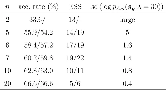
From Table 1, the efficiency of BSL and uBSL is very similar. The normalised ESS
suggests that n values of 5-7 give efficient results. However, we find that the posterior
results for n= 2 are slightly away from the other values of n for BSL.
Table 1: Sensitivity of BSL/uBSL to n for the simple example with regards to MCMC
acceptance rate and normalised ESS. Shown also is the estimated standard deviation of
the log SL at the true parameter value λ= 30. A ‘-’ indicates that a result is not available
for uBSL as the value of n is too small.
n acc. rate (%) ESS sd (logpA,n(sy|λ= 30))
2 33.6/- 13/- large
5 55.9/54.2 14/19 5
6 58.4/57.2 17/19 1.6
7 60.2/59.8 19/22 1.4
10 62.8/63.0 10/11 0.8
20 66.6/66.6 5/6 0.4
standard deviation. Despite this, BSL shows relatively high efficiency. Forn = 5 the tail is
less heavy but the standard deviation is well above 1. The standard deviation for n = 10
gives a value closer to that recommended of pseudo-marginal methods. However, n = 10
produces less efficient results than smaller values of n. The value of n = 20 produces
accurate synthetic likelihoods but requires too much computation to be useful.
4.1.2 Comparison to ABC
Using the squared difference between summary statistics as the discrepancy function, we
find that = 0.001 results in an ABC posterior close to the true posterior (see Figure
1(c)). The MCMC ABC acceptance probability is 17.2%. The normalised ESS for ABC is
25, indicating that ABC is more efficient than BSL and uBSL for this one parameter and
summary statistic example.
4.1.3 Normality
Here we investigate how the normality assumption of the BSL approaches affects the
ac-curacy of the results. The sum of N iidP(λ) variables is distributed asP(N λ). A general
rule of thumb is that a Poisson distribution is approximately normally distributed for mean
N = 100 with λ = 30 is chosen for an example where the normality assumption is
appro-priate andN = 10 with λ= 1 is chosen for an example where the normality assumption is
violated. For this investigation we use n = 50 and T = 100,000 so that any error can be
mostly attributed to the lack of normality of the summary statistic.
An Anderson-Darling test is performed using the summary statistic sample at each
MCMC iteration. Some graphs are displayed in Appendix F of the supplementary materials,
showing the accuracy of the estimated posterior along with some histograms of the p-values.
These graphs are shown for examples with λ = 1 and λ = 30. As expected, the p-values
do not appear to be uniformly distributed between zero and one in the example where
λ = 1. When λ = 30 the assumption of normality appears much more reasonable. The
BSL approaches appear to have very accurate estimates of the posterior distribution in
both cases, which is remarkable given the strong departure from normality when λ= 1.
4.2
Departure from Normality - Ricker Model
The summary statistics in this example are non-Gaussian so it is interesting to investigate
the sensitivity of BSL and uBSL to n and to compare their output with ABC, which does
not suffer from the multivariate normality assumption.
We consider the Ricker model presented in Wood (2010). Here a population of size Nt
at time t evolves according to Nt+1 = rNte−Nt+et where et iid
∼ N(0, σ2
e). However, a more
realistic scenario is where the Nt are unobserved and what is observed are the random
variables, Yt, such that Yt∼ P(φNt).
We set the model parameter asθ= (logr, φ, σe). The observed data of size N = 100 is
generated from the Ricker model with parameter θ = (3.8,10,0.3)> and N0 = 1. Here we
use the same summary statistics to that used in Wood (2010). These include the average
observation, the number of zeros, the autocovariances up to lag 5 (including the variance, lag
0), the parameter estimates of β0 andβ1 based on the regression,yt0.3 =β0yt0−.31+β1y0t−.61+ηt where ηt ∼ N(0, σ2η), and the coefficients of a cubic regression of the ordered differences on their observed values (see Wood (2010) for more details). This constitutes a total of 13
summary statistics. The prior distributions on the parameters are independent, uniform
To determine if the normality assumption of the summary statistic is reasonable, we
use the Anderson-Darling test for normality on each of the (marginal) summary statistics
when n= 100 for all values of θ proposed in MCMC BSL. We find that the components of
the summary statistic do not follow a normal distribution; there are departures away from
the uniform distribution for the p-values, significantly for many components (results not
shown). However, it does not appear that the distributions of the summary statistics are
highly irregular for θ with high posterior support, with some statistics showing skewness
without very heavy tails.
For this example, it is possible to use an unbiased particle filtering estimate of the
likelihood in particle MCMC (Andrieu et al., 2010) to target the posterior conditional on
the full data. Given that ABC and BSL work on the summary statistic level, a comparison
has not been included. See Fasiolo et al. (2016) who provide a comparison of particle
MCMC and BSL.
4.2.1 Sensitivity to n
To investigate the sensitivity of the BSL posteriors to n, we run the algorithm for a variety
of values of n. The results are shown in a table and in figures presented in Appendix G of
the supplementary materials. These figures demonstrate that the BSL target distributions
are again remarkably insensitive ton, given the lack of normality of the summary statistic.
Owing to the insensitivity of the target to n, the optimal n may be considered as the
one that maximises the normalised ESS. The efficiency of BSL and uBSL are again quite
similar. The optimal value of n out of the values tested appears to be 50 (with normalised
ESS values of 30, 35 and 45 for the three parameters), but values of n in the range 30-100
seem to provide relatively efficient results. For this range of n, values of the standard
deviation of the estimated log SL at the true parameter are roughly 1-4.
4.2.2 Comparison to ABC
We run ABC for 25 million iterations with an ABC tolerance that produces an acceptance
rate of roughly 0.26%. Our chosen ABC tolerance leads to normalised ESS values of 19,
3 3.5 4 4.5 0 1 2 BSL uBSL ABC ABC Reg
(a) logr
8 10 12
0 0.2 0.4 0.6 0.8 BSL uBSL ABC ABC Reg (b) φ
-0.2 0 0.2 0.4 0.6 0.8 1 0 1 2 3 4 BSL uBSL ABC ABC Reg
[image:19.612.110.506.74.253.2](c) σe
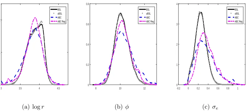
Figure 2: Posterior estimates for logr, φ and σe of the Ricker model when using ABC
(dash, based on 0.26% acceptance rate), ABC with regression adjustment (dot-dash), BSL
(solid) and uBSL (dot). The BSL approaches use n = 50. The online figure is in colour.
results with efficient n values. Regression adjustment is applied and appears to have a
small impact on all three parameters. This indicates that further reductions in may
have an effect on the ABC posterior, suggesting that BSL may be more efficient for this
example. There is some discrepancy between the (u)BSL and ABC posteriors for σe but
overall the BSL approaches produce an approximate posterior in the vicinity of the ABC
approximation despite the mild departure from normality of the summary statistics.
4.3
High Dimensional Summary Statistic - Cell Biology Model
In this realistic example, the summary statistic is of dimension 145. ABC suffers a curse
of dimensionality with respect to the size of the summary statistic, and intuitively one
might suspect that BSL will also suffer from a curse of dimensionality as the multivariate
normality assumption deteriorates in higher dimensions. The performance of ABC and
BSL in this application reveal how the methods scale with increasing dimension of the
summary statistic.
Cell motility and proliferation are important parts of many biological processes. Cell
motility causes random movement which, together with proliferation or reproduction, can
Zahm et al. (1997)). The main function of many medical treatments is to influence the
rates of these processes. In order to measure the efficacy of such treatments, it is important
that a measure of cell motility and proliferation can be accurately obtained. Unfortunately,
stochastic models for collective cell spreading do not possess a tractable likelihood function.
Several papers have adopted an ABC approach to estimate the parameters (e.g. Johnston
et al. (2014); Vo et al. (2015)). One difficulty with these cell biology applications is that
the observed data are typically available as sequences of images and therefore it is not
trivial to reduce the dimension of the summary statistic to a suitable level for ABC while
simultaneously retaining relevant information contained in the images.
A common method of collecting information about cell diffusivity and proliferation is
the scratch assay (e.g. Fronza et al. (2009); Johnston et al. (2014)). Scratch assays can
be used to measure cell migration in vitro and can be performed with readily available
and inexpensive equipment. Once cells have formed a single layer completely covering the
assay (i.e. a confluent monolayer), a ‘scratch’ is made which separates the cells (Liang
et al., 2007). Images of the cells are taken at regular time intervals until the cells are once
again in contact, and often the images are then reduced to summary statistics. In most
cases (e.g. Johnston et al. (2014); Treloar and Simpson (2013); Simpson et al. (2013)),
formal analysis is performed on a small number of images with intervals of at least one
hour, even when images are taken more frequently. In the experiment of Johnston et al.
(2014), images of murine fibroblast cells (3T3 cells) are taken every 5 minutes for 12 hours
and here we consider the possibility of using all 145 images (including the initial image) in
the analysis. Johnston et al. (2014) consider 3 of these images, at 4, 8 and 12 hours. By
using 145 images rather than a small subset of this, valuable information about the rates
of motility and proliferation could be attained. Here we investigate the capabilities of BSL
to accommodate this high-dimensional summary statistic and compare it with ABC with
the same summary statistic and also with the ABC approach of Johnston et al. (2014) who
consider only 3 images. The reader is referred to Johnston et al. (2014) for the summary
statistics used in their article.
To create the observed data, the cells can be placed on a two-dimensional discrete
process and part of the reason why Johnston et al. (2014) consider only 3 images (in
addition to reducing the dimensionality of the problem). Here we consider simulated data
to determine whether it might be beneficial to manually process more images, in terms of
how much additional information is obtained about the parameters. Let Xt
x,y ∈ {0,1} be an indicator that defines whether a cell is present at position (x, y) for x ∈ {1, . . . , R},
y∈ {1, . . . , C}at time indext ∈ {0,1, . . . ,144}. HereRandC are the number of rows and
columns in the lattice, respectively. Denote the matrix of indicators at time index tas Xt.
One possibly informative summary statistic regarding motility is the Hamming distance
between Xt and Xt−1
st= R X
x=1
C X
y=1
|Xx,yt −Xx,yt−1|.
This summary statistic should be suitable if relatively few motility events take place during
the time interval since the Hamming distance does not take into account how far cells might
have travelled, only the number of positions in the two matrices that differ. The summary
statistic we use to provide information regarding the proliferation is the total number of
cells at the end of the experiment, which we denote asK for some simulated dataset. Thus
the simulated summary statistic is given by s= (s1, . . . , s144, K) and is of dimension 145.
Random walk models allow for the direct comparison of simulations to their observed
counterparts. The random walk used here is a reflection of the cells under consideration.
Cells are motile, with the ability to move to a neighbouring lattice site (north, east, south,
west) during each time period of duration τ, which is fixed and set small enough so it
approximates well a stochastic process in continuous time. Assuming that there are a
total of N(t) cells present at time t, then during each time step N(t) cells are chosen with
replacement and given the opportunity to move (Simpson et al., 2013). Experiments have
suggested that the cell movement is random, so cells are equally likely to attempt movement
in thex and ydirections. If the attempted movement is to a vacant site, then the motility
event is successful.
When 3T3 fibroblast cells proliferate, they have a separation distance of one (Simpson
et al., 2010). After all motility events have been attempted during a single time step, N(t)
cells are chosen with replacement and given the opportunity to proliferate. The proliferation
The outcomes of this biological process are determined solely by the cell motility and
proliferation so only two parameters are required in the random walk. While the parameters
of interest are the diffusivity D and the proliferation rate λ, it is simple to just work with
the probabilities of motility and proliferation, Pm ∈[0,1] and Pp ∈[0,1]. Conversion back
to the biological parameters is done by using the formulae in Johnston et al. (2014). It is
also possible to include additional parameters for cell-to-cell adhesion and cell-to-substrate
adhesion depending on the type of cell under consideration. For more details on the random
walk simulation model, the reader is referred to Johnston et al. (2014).
The data are simulated with Pm = 0.35 and Pp = 0.001 with R = 27 and C =
36. Initially, N(0) = 110 cells are placed randomly in the rectangle with positions x ∈
{1,2, . . . ,13}and y∈ {1,2, . . . ,36}.
4.3.1 Sensitivity to n
We run the BSL methods with various values of n, with the table of results and the
estimated BSL and uBSL posteriors for different values of n given in Appendix H of the
supplementary materials. It is again remarkable how insensitive the (u)BSL posteriors are
ton, given the high-dimensional summary statistic. Despite this insensitivity of the target
ton, very large values ofnare required to estimate the SL precisely and achieve reasonable
mixing due to the high dimensional summary statistic. However, we are able to take
advantage of the embarrassingly parallel nature of BSL by performing the n independent
model simulations on a computer node with 16 cores. This is trivial to implement, using
the parfor technology in Matlab, for example.
The BSL and uBSL methods have similar efficiency. The optimal value ofn appears to
be n = 5000 which produces an estimated log SL of 1.4. However, n values between 2500
and 10000 are also relatively efficient.
4.3.2 Comparison to ABC
We run ABC with the same set of summary statistics. We make use of the 16 processors
by taking the average of the kernel weighting function values for 16 independent model
0.1 0.2 0.3 0.4 0.5 0.6 0
10 20 30 40 50 60 70
ABC 3 images ABC all images ABC all images reg adj BSL all images
(a) Pm
×10-3
0 1 2
0 1000 2000 3000
ABC 3 images ABC all images ABC all images reg adj BSL all images
[image:23.612.115.498.77.319.2](b) Pp
Figure 3: Posterior density estimates for (a) Pm and (b) Pp of the collective cell spreading
model when using the ABC approach of Johnston et al. (2014) (solid), ABC with all the
images without (dot-dash) and with (dot) regression adjustment, and BSL (n = 5000)
with all the images (dash). Shown in squares with a vertical line are the true values of the
parameters used to generate the data. The online figure is in colour.
ABC is run with several different tolerance values within = 1000 and = 1500. These
choices of the tolerances result in acceptance rates between 1% and 8%. The tolerance of
= 1000 produces normalised ESS values closest to the BSL approaches with near optimal
n. However, we find that this tolerance leads to poor (non-smooth) posterior density
estimates even after significant thinning. We suggest that the very low acceptance rate is
leading to an inaccurate estimate of the ESS. The tolerance of = 1100 gives smoother
posterior estimates. We also perform regression adjustment. In the regressions we use
the first discrepancy value and associated simulated summary statistic produced by the 16
independent simulations at each iteration of MCMC ABC.
The comparison of the posterior results for ABC, BSL (n = 5000) and the ABC
ap-proach of Johnston et al. (2014) is shown in Figure 3. The results for uBSL and BSL
that a substantial amount of additional information can be obtained about the motility
parameter Pm by considering more than 3 images. Further, the results from BSL are much
more precise than that from ABC (cross-validation provides reassurance that we are not
over-confident in the parameter values, see Appendix H of the supplementary materials).
Remarkably, the ABC results using 3 images are much more precise than the ABC results
for Pp (Figure 3(b)) using all the images. Note that Johnston et al. (2014) consider the
number of cells at each of the three time points (including 12 hours). Both BSL and ABC
with all the images use the number of cells at 12 hours as a summary statistic. The
re-sults for Pp from BSL are very close to the results of the ABC approach of Johnston et al.
(2014). It appears that ABC with all the images is being greatly affected by the inability
to reduce the ABC tolerance, further demonstrated by the strong impact of the regression
adjustment.
The BSL approaches are able to make use of the multiple cores in a more efficient
manner than ABC. Given the much higher acceptance rates of MCMC BSL compared to
ABC, fewer iterations are required which implies fewer calls to the multiple cores. Further,
due to the large value of n required to estimate the BSL target precisely, the multiple
cores are given a significant amount of work to do. ABC performs on average 67 model
simulations per second, whereas BSL is able to produce 820 model simulations per second.
It appears that BSL, together with the capabilities of parallel computing, is able to deal
with the very high-dimensional summary statistic in this application.
5
Discussion
Our empirical results suggest that the optimal value of the standard deviation of the
es-timated log SL (at a parameter value with high posterior support) is likely to be above
1, the value recommended generally for pseudo-marginal methods (Doucet et al., 2015).
However, in their theoretical results, Doucet et al. (2015) assume that the log-likelihood
estimator has a normal distribution. For BSL we observe that for moderate values of n
the synthetic log-likelihood estimator can have a heavy left tail (i.e. underestimated
syn-thetic log-likelihoods). This might explain the larger optimal standard deviation that we
log-likelihood does not cause much problem in pseudo-marginal methods as these values
are simply rejected. More concerning is when the log-likelihood estimator has a heavy
right tail, which can result in the likelihood being grossly overestimated and the MCMC
chain becoming stuck at that value for a long period. We do note that the BSL target is
remarkably insensitive to n and there appears to be quite a large range of n values that
lead to relatively efficient results (an estimated log SL of between 1 and 3, roughly). These
results indicate that it may be easier to select a value of n in BSL compared to selecting
in ABC. Even when there are significant departures in normality of the summary statistic,
but where the distribution of the summary statistic remains regular, BSL can still produce
reasonable approximations. However, when the distribution of the summary statistic is
highly irregular as in the example given in Appendix I of the supplementary materials, the
output of BSL cannot be trusted, whilst ABC represents a robust alternative in such cases.
We find that even though uBSL has an estimated log SL with infinite variance, in
practice it gives an efficiency that appears similar to BSL. Further, we find in the examples
that BSL and uBSL provide similar posterior approximations. Despite the fact the uBSL
provides some additional theoretical support in terms of the sensitivity of the posterior
approximation to n, we find that the standard BSL posterior is remarkably insensitive to
n. Given this, it may be that the standard BSL method is adopted more often in future
applications as it is simpler to implement.
In a serial computing environment, some theoretical results suggest that BSL should
be more computationally efficient than ABC when the dimension of the summary statistic
is greater than 2. ABC is known to suffer from the curse of dimensionality, and this may
also be a concern in BSL with the multivariate normal approximation deteriorating in
higher dimensions. However, the theoretical results in favour of BSL are supported by
empirical results which demonstrate that BSL becomes increasingly efficient relative to
ABC as the dimension of the summary statistic increases. Since the optimal value of n
in BSL is inherently greater than 1, BSL may benefit more from parallel computing than
ABC, where the optimal number of replicated simulations is n = 1 in a serial computing
environment (Bornn et al., 2016). In the cell biology application we found an order of
Meeds and Welling (2014) develop an approach that adaptively chooses the value ofnat
each iteration in order to keep the probability of making an incorrect accept/reject decision
below a chosen level. When one parameter configuration is clearly preferred over another,
only a small value of n is required. Given the insensitivity of the target distribution to n,
such an approach may be useful for further improving the efficiency of the BSL approaches.
One aspect of the MCMC BSL approaches we have not investigated is the convergence
properties. We found that when the chain is initialised in a negligible point of the posterior
support that it can become stuck there for long periods. In these parts of the space the
SL is estimated with very high variability. Lee and Latuszy´nski (2014) show that the ABC
MCMC kernel that we use in this paper is not geometrically ergodic. It would be interesting
to explore the convergence properties of the MCMC BSL approaches. Some studies have
investigated the asymptotic properties of various ABC methods (e.g. Li and Fearnhead
(2016) and Frazier et al. (2016)). Further research on the asymptotic properties of BSL
would be of interest.
We have done some initial investigations on the performance of BSL when the model is
misspecified. Specifically, when the model is unable to recover the observed statistic, sy.
We found that a larger value of n than what might be expected for a given dis required to
achieve a reasonable acceptance probability in MCMC (u)BSL and that the BSL methods
are not necessarily robust to such misspecifications. The reason for the poor efficiency is
thatsyis always in the tails of the SL and is thus harder to estimate. It is possible that ABC
may be more robust and efficient in such settings, but this requires further investigation.
However, these scenarios would typically motivate further model development.
Higher variability in the tails of the SL is a general issue affecting convergence and
caus-ing the algorithm to become stuck, especially in cases of model misspecification and highly
irregular summary statistics. To help overcome these issues, a parametric auxiliary model
other than the multivariate normal can be used which is equivalent to working in the
gen-eral psBIL framework. One possible avenue for further research is to investigate the use of
a multivariate-t auxiliary model for the summary statistic to improve the robustness of the
method. However, the multivariate-t distribution does not have a convenient closed form
summary other than normal could be handled using a Gaussian copula model. It would
be possible in this framework to consider semi-parametric models where the marginals are
fitted using kernel density estimates and the dependence between marginals modelled with
a Gaussian copula.
The major issue with estimating the SL precisely is in estimating the covariance matrix
of the summary statistic accurately. The sample covariance matrix used in this paper is an
unbiased estimator but it is well known that there are biased but lower variance estimators
particularly in the presence of small samples (see Ledoit and Wolf (2004) and Friedman
et al. (2008)). We plan to investigate such approaches in future research, which may lead
to BSL methods that require fewer model simulations.
Following MCMC ABC, a series of sequential Monte Carlo (SMC) ABC approaches (e.g.
Sisson et al. (2007)) have been developed that appear to increase efficiency. The major
advantages of the SMC approach over MCMC ABC is that it is straightforward to adapt
the parameter proposal in this framework, a population of particles prevents the algorithm
from getting stuck and many of the algorithms have natural stopping rules so that does
not need to be explicitly chosen (e.g. Vo et al. (2015)). Further, SMC can facilitate fully
Bayesian model comparisons more easily than in MCMC (see, for example, Drovandi and
McCutchan (2016)). Everitt et al. (2016) use BSL within an SMC framework to perform
model comparisons in models with intractable normalising constants. There is scope to
extend this algorithm, for example to develop an exact-approximate SMC BSL algorithm
and to adaptively select the value of n as the sequence of targets is traversed.
Overall the BSL approaches appear to be useful methods for approximating p(θ|sy).
The method requires less tuning than ABC, is more computationally efficient than ABC in
challenging scenarios, shows some robustness to the normality assumption and is
embar-rassingly parallelisable. The clear drawback of the method is the normality assumption,
which will be increasingly violated with an increasing dimension of the summary
statis-tic. Although our paper suggests that BSL remains an interesting avenue to investigate,
further research on the theoretical properties of the method is required and to determine
6
Supplementary Material
Additional information to supplement the main paper is available in the following files
found online.
Appendices: Contains all appendices to the main document. (Appendices.pdf, PDF
portable document format)
Code: Contains all of the code required to perform the described methods on the Ricker
example from Section 4.2. (Code.zip, compressed (zipped) folder)
References
Andrieu, C., A. Doucet, and R. Holenstein (2010). Particle Markov chain Monte Carlo methods. Journal of the Royal Statistical Society: Series B (Statistical
Methodol-ogy) 72(3), 269–342.
Andrieu, C. and G. O. Roberts (2009). The pseudo-marginal approach for efficient Monte Carlo computations. The Annals of Statistics 37(2), 697–725.
Beaumont, M. A. (2003). Estimation of population growth or decline in genetically moni-tored populations. Genetics 164(3), 1139–1160.
Beaumont, M. A., W. Zhang, and D. J. Balding (2002). Approximate Bayesian computation in population genetics. Genetics 162(4), 2025–2035.
Blum, M. G. B. (2010). Approximate Bayesian computation: a non-parametric perspective.
Journal of the American Statistical Association 105(491), 1178–1187.
Blum, M. G. B., M. A. Nunes, D. Prangle, and S. A. Sisson (2013). A comparative review of dimension reduction methods in approximate Bayesian computation.Statistical
Science 28(2), 189–208.
Bornn, L., N. S. Pillai, A. Smith, and D. Woodard (2016). The use of a single pseudo-sample in approximate Bayesian computation. To appear in Statistics and Computing.
Brown, V. L., J. M. Drake, H. D. Barton, D. E. Stallknecht, J. D. Brown, and P. Rohani (2014). Neutrality, cross-immunity and subtype dominance in avian influenza viruses.
PLOS ONE 9(2), 1–10.
Dale, P. D., P. K. Maini, and J. A. Sherratt (1994). Mathematical modeling of corneal epithelial wound healing. Mathematical Biosciences 124, 127–147.
Doucet, A., M. K. Pitt, G. Deligiannidis, and R. Kohn (2015). Efficient implemen-tation of Markov chain Monte Carlo when using an unbiased likelihood estimator.
Biometrika 102(2), 295–313.
Drovandi, C. C. and R. A. McCutchan (2016). Alive SMC2: Bayesian model selection for
low-count time series models with intractable likelihoods. Biometrics 72, 344–353.
Drovandi, C. C., A. N. Pettitt, and A. Lee (2015). Bayesian indirect inference using a parametric auxiliary model. Statistical Science 30(1), 72–95.
Everitt, R. G., A. M. Johansen, E. Rowing, and M. Evdemon-Hogan (2016). Bayesian model comparison with un-normalised likelihoods. To appear in Statistics and Computing.
Fasiolo, M., N. Pya, and S. N. Wood (2016). A comparison of inferential methods for highly non-linear state space models in ecology and epidemiology. Statistical Science 31(1).
Fasiolo, M. and S. N. Wood (2016). To appear in Handbook of Approximate Bayesian
Computation, Chapter Approximate methods for dynamic ecological models.
Frazier, D. T., G. M. Martin, C. P. Robert, and J. Rousseau (2016). Asymptotic properties of approximate Bayesian computation. https://arxiv.org/pdf/1607.06903.pdf.
Friedman, J., T. Hastie, and R. Tibshirani (2008). Sparse inverse covariance estimation with the graphical lasso. Biostatistics 9(3), 432–441.
Fronza, M., B. Heinzmann, M. Hamburger, S. Laufer, and I. Merfort (2009). Determination of the wound healing effect of Calendula extracts using the scratch assay with 3T3 fibroblasts. Journal of Ethnopharmacology 126(3), 463–467.
Ghurye, S. G. and I. Olkin (1969). Unbiased estimation of some multivariate probability densities and related functions. The Annals of Mathematical Statistics 40(4), 1261–1271.
Gutmann, M. U. and J. Corander (2015). Bayesian optimization for likelihood-free infer-ence of simulator-based statistical models. To appear in Journal of Machine Learning
Research.
Hartig, F., C. Dislich, T. Wiegand, and A. Huth (2014). Technical note: approximate Bayesian parameterization of a process-based tropical forest model. Biogeosciences 11, 1261–1272.
Johnston, S., M. J. Simpson, D. L. S. McElwain, B. J. Binder, and J. V. Ross (2014). Interpreting scratch assays using pair density dynamic and approximate Bayesian com-putation. Open Biology 4(9), 140097.
Jones, D. R. (2001). A taxonomy of global optimization methods based on response surfaces.
Ledoit, O. and M. Wolf (2004). A well-conditioned estimator for large-dimensional covari-ance matrices. Journal of Multivariate Analysis 88(2), 365–411.
Lee, A. and K. Latuszy´nski (2014). Variance bounding and geometric ergodicity of Markov chain Monte Carlo kernels for approximate Bayesian computation. Biometrika 101(3), 655–671.
Li, W. and P. Fearnhead (2016). Improved convergence of regression adjusted approximate Bayesian computation. https://arxiv.org/pdf/1609.07135.pdf.
Liang, C.-C., A. Y. Park, and J.-L. Guan (2007). In vitro scratch assay: a convenient and inexpensive method for analysis of cell migration in vitro. Nature Protocols 2(2), 329–333.
Marin, J.-M., P. Pudlo, C. P. Robert, and R. J. Ryder (2012). Approximate Bayesian computation methods. Statistics and Computing 22(6), 1167–1180.
Meeds, E. and M. Welling (2014). GPS-ABC: Gaussian process surrogate approximate Bayesian computation. In Proceedings of the Thirtieth Conference Annual Conference
on Uncertainty in Artificial Intelligence (UAI-14), Corvallis, Oregon, pp. 593–602. AUAI
Press.
Moores, M. T., C. C. Drovandi, K. L. Mengersen, and C. P. Robert (2015). Pre-processing for approximate Bayesian computation in image analysis. Statistics and
Com-puting 25(1), 23–33.
Plummer, M., N. Best, K. Cowles, and K. Vines (2006). CODA: convergence diagnosis and output analysis for MCMC. R News 6(1), 7–11.
Rayner, G. D. and H. L. MacGillivray (2002). Numerical maximum likelihood estimation for the g-and-k and generalized g-and-h distribution. Statistics and Computing 12(1), 57–75.
Simpson, M. J., K. A. Landman, and B. D. Hughes (2010). Cell invasion with proliferation mechanisms motivated by time-lapse data. Physics A: Statistical Mechanics and its
Applications 389, 3779–3790.
Simpson, M. J., K. K. Treloar, B. J. Binder, P. Haridas, K. J. Manton, D. I. Leavesley, D. L. S. McElwain, and R. E. Baker (2013). Quantifying the roles of cell motility and cell proliferation in a circular barrier assay. Journal of the Royal Society Interface 10(82), 20130007.
Sisson, S. A. and Y. Fan (2011). MCMC handbook, Chapter Likelihood-free Markov chain Monte Carlo, pp. 313–335. Chapman & Hall.
Swanson, K. R., C. Bridge, J. D. Murray, and E. C. A. Jr (2003). Virtual and real brain tumor: using mathematical modeling to quantify glioma growth and invasion. Journal
of the Neurological Sciences 216, 1–10.
Treloar, K. K. and M. J. Simpson (2013). Sensitivity of edge detection methods for quan-tifying cell migration assays. PLoS ONE 8(6), e67389.
Vo, B. N., C. C. Drovandi, A. N. Pettitt, and G. J. Pettet (2015). Melanoma cell colony expansion parameters revealed by approximate Bayesian computation. PLOS
Computa-tional Biology 11(12), e1004635.
Vo, B. N., C. C. Drovandi, A. N. Pettitt, and M. J. Simpson (2015). Quantifying un-certainty in parameter estimates for stochastic models of collective cell spreading using approximate Bayesian computation. Mathematical Biosciences 263, 133–142.
Wilkinson, R. (2014). Accelerating ABC methods using Gaussian processes. Journal of
Machine Learning Research 33, 1015–1023.
Wood, S. N. (2010). Statistical inference for noisy nonlinear ecological dynamic systems.
Nature 466, 1102–1107.