Zone-based, Robust Flood Evacuation Planning
ISabine B¨uttnera, Marc Goerigkb,∗
aTechnische Universit¨at Kaiserslautern, Kaiserslautern, Germany bUniversity of Lancaster, Lancaster, United Kingdom
Abstract
We consider the problem to evacuate several regions due to river flooding, where suffi -cient time is given to plan ahead. To ensure a smooth evacuation procedure, our model includes the decision which regions to assign to which shelter, and when evacuation orders should be issued, such that roads do not become congested.
Due to uncertainty in weather forecast, several possible scenarios are simultane-ously considered in a robust optimization framework. To solve the resulting integer program, we apply a Tabu search algorithm based on decomposing the problem into better tractable subproblems. Computational experiments on random instances and an instance based on Kulmbach, Germany, data show considerable improvement com-pared to an MIP solver provided with a strong starting solution.
Keywords: Evacuation Planning, Flood Evacuation, Robust Optimization
1. Introduction
World-wide, flood damages have been on the rise and will likely continue to pose a further increasing risk. The floods in June 2013 are estimated to amount to 12 billion Euro in losses [Re13], while the floods in India and Pakistan during September 2014 caused over 5 billion US$ and 665 fatalities alone [Re14]. Yearly losses within the EU are estimated to increase to over 23 billion Euro annually by 2050 [JHSF+14].
Due to highly sophisticated weather forecasts, floods do not hit us completely by surprise, and do not belong to the class of no-notice emergencies. Therefore, opera-tions research has great potential to prepare for and to mitigate flood effects. Still, the literature on optimization models specifically for flood evacuation has been relatively sparse so far in comparison to other natural disasters [AG06]; for general surveys on evacuation planning and disaster management, we refer to [HT01, AG06].
IPartially supported by the German Ministry of Research and Technology (BMBF), project
RobEZiS, grant number 13N13198.
∗Corresponding author; Address: Lancaster University Management School, Bailrigg, Lancaster,
LA1 4YX, United Kingdom; Phone:+44 (0)1524 595125
In [KYC05], a game-theoretic model for shelter location and allocation in flood evacuation planning is presented, which amounts to a bi-level optimization program that is solved using a genetic algorithm. Other papers include data uncertainty by developing robust and stochastic optimization models. In [CTC07], a two-stage pro-gram for flood evacuation is presented that includes the location of storehouses and the allocation and distribution of resources. To solve this model, sample average approx-imation is applied. A robust model for issuing evacuation instructions is presented in [HHH11], which extends the previous work [HHPB10]. An ant colony algorithm is applied to solve the model.
Robust optimization has been successfully applied also to other problems in disas-ter management, e.g., in [GDT15, GG14, KWLY11]. For general overviews on robust optimization, see [KY97, ABV09, BTGN09, GS15].
In this paper we present a model for planning an evacuation due to inland flooding, that takes the decision when to issue the evacuation orders, and the assignment of regions to shelters into account. In Section 2 we discuss this model in detail, before presenting a formulation as an integer program (IP) and showing itsN P-hardness in Section 2.2. Acknowledging the data uncertainty present in our problem, we discuss a robust model extension in Section 3. To solve this model, we consider a decomposition of the problem in Section 4 and a Tabu search heuristic in Section 5. Our solution algorithms are tested in computational experiments that are described in Section 6. Section 7 concludes our paper and points to further areas of research.
2. Nominal Model Definition
2.1. Model Purpose and Description
To simplify the presentation, we first introduce our flood evacuation model with-out data uncertainty, i.e., when weather forecasts are reliable. We then extend this formulation to several scenarios in Section 3.
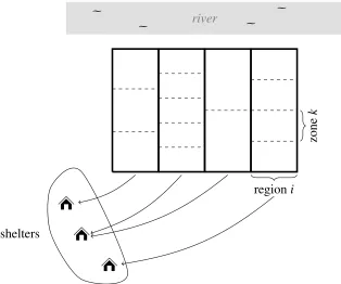
Consider the following evacuation problem, which we denote as the flood evac-uation problem (FEP): in foresight of a river flooding, an evacevac-uation plan has to be determined for a certain landscape (e.g. a city) consisting of an assignment of the evacuees to one of a number of available shelters and, additionally, an (individual) evacuation order, i.e. a time at which the instruction to evacuate is issued. The area of consideration is divided into certainregions(e.g. quarters) and each of the regions itself is subdivided into severalzones(e.g. blocks), see also Figure 1.
leave a certain time span later than receiving the instruction. Hence, a certainresponse timecan be observed.
Finally, in the situation of a river flooding, not all areas are exposed to the same risk from a chronological view. Some areas are flooded earlier than others (those lying upstream and those closer to the river.)
To incorporate all of these properties we propose the following model (in discrete time-steps): The regions within the area to be evacuated and the zones within each region as well as the set of available shelters are known. For each of the zones, there is a latest notification time at which the evacuation order should be issued at latest. The violation of these target times will be the criterion when determining an optimal evacuation plan. Furthermore, the total number of evacuees in a zone (the demand) is known but, moreover, we know theresponse profileof the zone: the total demand is split into the number of people leaving directly after receiving the evacuation order, the number leaving one time step after that, two time steps delayed, etc. This profile is given independently for each zone. This allows to model the fact that usually an evacuee living closer to the waterside will leave earlier than somebody living more inland and we assume these values to be fixed (e.g. estimated due to evacuees’ behavior in earlier flooding situations).
For each of the shelters two values are given: on the one hand the totalcapacity
giving the maximum number of people assigned to the same shelter, and on the other hand also an accommodation rategiving the maximum number of people arriving at the shelter per time step. Both capacity constraints are strict. Due to budgeting reasons, not all available shelters can be used; instead, there is a bound given on the number of shelters that may be opened.
Then, a feasible evacuation plan determines an assignment of the regions to the shelters and an evacuation order time individually for each zone such that the overall capacity of no shelter is exceeded and the number of evacuees arriving at a shelter at the same time does not exceed the accommodation rate. In particular, all evacuees from the zones within one region are assigned to the same shelter, but a shelter can host evacuees from several regions (as long as both the overall capacity restriction and – at each time – the bound on the number of arriving evacuees from all regions w.r.t. the respective evacuation orders times and the response profile is fulfilled).
The plan is considered optimal if the number of evacuees being informed (and thus evacuated) later than their respective target time is minimal.
river
e
e e
e
regioni
zone
k
shelters
Figure 1: The zonal model (FEP).
0 5 10 15 20
1 2 3 4 5 6 7 8 9 10111213
d
1
time
(a) Response profiled1.
0 5 10 15 20
1 2 3 4 5 6 7 8 9 10 12 13
d
2
time
(b) Response profiled2.
0 5 10 15 20
1 2 3 4 5 6 7 8 9 10111213
d
1 + d
2
time
[image:4.612.128.442.107.369.2](c) Combined response pro-file, if d2 is delayed by three time units.
Figure 2: Example for response profiles with feasible evacuation order when the accommodation rate is 20.
2.2. IP formulation
We now describe an integer programming model for (FEP), beginning with data and variables in Section 2.2.1, followed by objectives and constraints in Section 2.2.2.
2.2.1. Data and Variables
The following sets are given in the (FEP):
• zonesKi = {1, . . . ,ki}for each regioni∈I,
• sheltersS={1, . . . ,m}.
For each zonek ∈Kiwe have:
• response profile [dik
0, . . . ,d
ik
tk], where d ik
t is the demand in zone k, in t periods
after the evacuation order is given.
Dikis the overall demand in zonekandD
idenotes the overall demand of regioni,
that is Dik
BP0≤τ≤tkd
ik
τ andDi BPk∈Ki D ik,
• desired notification time ∆ik until which the evacuation order should be issued.
The desired notification time should be chosen in a way that, depending on the respective response profile, all evacuees have left the region before being endan-gered.
For each shelter j∈ Swe have:
• capacity uj, giving the maximum number of evacuees in shelter j,
• accommodation rate bj, the maximum number of evacuees arriving at jper
pe-riod.
Additionally, we have:
• time horizon T ∈N. We setT ={1, . . . ,T}.
• maximum number of shelters C, denoting the number of shelters fromSthat can be used.
Finally, we assume when any evacuation order is given within the time horizonT0 ⊆
T, there is sufficient time available withinT for the evacuation to be completed (for the simplicity of notation, we assumeT0
to be the same for all regions and zones). We furthermore introduce the following variables:
• zi j ∈ {0,1} =: B to model if the evacuees from region i ∈ I are assigned to
shelter j∈ S
• xikt ∈Bto model if the evacuation order for zonek∈ Ki in regioni ∈ Iis given
at timet ∈ T0
• sj ∈Bto model if shelter j∈ Sis opened
• yikt j ∈ N is the number of evacuees leaving zone k ∈ Ki in region i ∈ I to
2.2.2. Integer Program
Using the above notation, we formulate the (FEP) as follows:
min X
i∈I
X
k∈Ki
X
τ∈T 0
τ≥∆ik
(τ−∆ik)·xikt (1)
s.t. X
t∈T0
xikt =1 for alli∈ I,k∈ Ki (2)
X
j∈S yikt j =
X
τ≤t
dτikxik(t−τ) for alli∈ I,k∈ Ki,t ∈ T (3)
X
j∈S
zi j = 1 for alli∈ I (4)
X
t∈T
yikt j ≤ zi jM for alli∈ I,k∈ Ki, j∈ S (5)
X
i∈I
zi jDi ≤ujsj for all j∈ S (6)
X
i∈I
X
k∈Ki
yikt j ≤bjsj for all j∈ S,t∈ T (7)
X
j∈S
sj ≤C (8)
xikt ∈B for alli∈ I,k∈ Ki,t ∈ T
0
(9)
zi j ∈B for alli∈ I, j∈ S (10)
sj ∈B for all j∈ S (11)
yikt j ∈N for alli∈ I,k∈ Ki,t ∈ T, j∈ S (12)
The constant parameterMin constraint (5) is chosen sufficiently large, e.g.M= P
iDi.
The objective (1) is to minimize the number of evacuees who are evacuated too late with respect to the respective notification time∆ik (weighted with the severity of
the delay). Note that if the evacuation order is issued before∆ik, then the
correspond-ing term in the objective becomes zero; for delayed evacuation orders, the penalty increases linearly.
A solution of the IP encodes a solution to the (FEP): for each zone, exactly one evacuation order is issued (2) and the number of evacuees leaving a zone are com-puted accordingly (3). All evacuees are assigned to one shelter (4) and, moreover, all evacuees from one region are assigned to the same shelter (5). The maximum capacity of each shelter is not exceeded (6) and, at no time, more than the allowed number of evacuees arrive at a shelter (7). Finally, Constraint (8) ensures that at mostCshelters are being used.
2.3. Hardness
3-partition
instance: A = {a1, . . . ,a3m}whereai ∈Z,Piai = mBand B4 < ai < B2 for
alli.
question: Can A be partitioned into disjoint sets A1, . . . ,Am such that
P
a∈Aja= Bfor all j?
Given an instance of 3-partition, we construct an instance of (FEP) as follows:
there are 3m regions with only one zone each. The response profile of this zone in regioniis [ai], i.e. there is no delayed response but all evacuees leave right after
re-ceiving the order. The target time is∆ = m−1 for all zones, s.t. the best objective value equals 0 if and only if there is a solution in which all zones receive the evacuation order within the firstmtime steps. Additionally there is a single shelter with capacity 3mand accommodation rate B. The time-horizon is sufficiently large. Note that this construction can be done in polynomial time.
Then, a solution with objective value equal to zero is equivalent to a partition of the set A into triples of weight B and, hence, solving (FEP) allows answering the
3-partitionproblem. As 3-partition is N P-hard in the strong sense (cf. [GJ79]), this
also holds for the (FEP).
2.4. Determining the Time Horizon
We now discuss how the parameterT can be found such that it is large enough to allow a feasible solution to (FEP); at the same time, finding the smallest possible such
T improves the computational performance when solving (FEP).
To this end, letlikdenote the length of the evacuation profiledik, i.e.,
lik =max
n
t∈ T :dikt >0
o
−minnt∈ T :dikt >0
o .
For each shelter j0 ∈ S, we solve a subproblem that determines the maximum sum of such lengths that can be feasibly assigned to j0. Letd
i = maxk∈Kimaxt∈Td ik
t . For fixed j0, the optimization problem we consider is given by
maxX
i∈I
X
k∈Ki
likzi j0 (13)
s.t. X
j∈S
zi j = 1 for alli∈ I (14)
X
i∈I
Dizi j ≤ujsj for all j∈ S (15)
dizi j ≤ bjsj for all j∈ S (16)
X
j∈S
sj ≤C (17)
zi j ∈B for alli∈ I, j∈ S (18)
As before, Constraints (14) ensure that every region is assigned to one shelter, while Constraints (15) and (16) model that both shelter capacity and shelter accommodation rate are respected. Constraint (17) bounds the number of shelters that can be opened byC. The objective function (13) aims at finding the worst-case over all assignments to j0. Solving (13–19) for all shelters, and taking the maximum of all optimal values, then gives an upper bound on the value ofT.
3. The Robust Problem
We now extend the nominal (FEP) model from Section 2.2 to include data uncer-tainty. To this end, we assume the following setting:
As the severity of a flood cannot be forecasted with complete certainty, there are different scenarios possible, which should all be taken into account during the planning step. The set of possible scenarios is called the uncertainty setU. The flood severity affects both the evacuation profiled and the desired order issue time∆, such that we set
U= n(d1,∆1), . . . ,(dN,∆N)o
The assignment of regions to shelters is a question of long-term planning, and should be done well in advance of the actual evacuation (e.g., shelters must be equipped for the right number of evacuees, endangered regions must be informed which path to use during an evacuation, etc.). Hence, the decision variables zi j and sj must be the
same for all scenarios. However, the actual time of notification for the evacuation or-der can be adapted to the circumstances; hence, variablesxikt andyikt jmay be decided
upon once the scenario is known to the planner. We therefore adapt a two-stage setting, and use sets of variablesxξ andyξ for each scenario.
We now present an IP formulation using the resulting robust model, which we call (RFEP). We setN :={1, . . . ,N}.
min ζ (20)
s.t. ζ≥ X
i∈I
X
k∈Ki
X
τ∈T 0
τ≥∆ξ
ik
(τ−∆ξ
ik)·x
ξ
ikt for allξ∈ N (21)
X
t∈T0
xξikt = 1 for alli∈ I,k∈ Ki, ξ ∈ N (22)
X
j∈S
yξikt j = X
τ≤t
dikτξxξik(t−τ) for alli∈ I,k∈ Ki,t ∈ T, ξ ∈ N (23)
X
j∈S
zi j = 1 for alli∈ I (24)
X
t∈T
yξikt j ≤ Mzi j for alli∈ I,k∈ Ki, j∈ S, ξ ∈ N (25)
X
i∈I
X
i∈I
X
k
yξikt j ≤ bjsj for all j∈ S,t∈ T, ξ∈ N (27)
X
j∈S
sj ≤C (28)
xiktξ ∈B for alli∈ I,k∈ Ki,t ∈ T, ξ ∈ N (29)
zi j ∈B for alli∈ I, j∈ S (30)
sj ∈B for all j∈ S (31)
yξikt j ∈N for alli∈ I,k∈ Ki,t ∈ T, j∈ S, ξ ∈ N (32)
ζ≥ 0 (33)
The new variable ζ is used to determine the worst-case over all scenarios with the help of Constraints (21). The remaining Constraints (22–33) are a direct extension of Constraints (2–12). Note that (RFEP) is alsoN P-hard, containing (FEP) as a special case.
4. Problem Decomposition
To better access model (RFEP) using heuristic solution approaches, we decompose the problem into two subproblems: Firstly, to find a feasible assignment of regions to shelters; and secondly, to find a good set of evacuation order times for all zones assigned to a fixed shelter and under a fixed scenario.
4.1. Finding a Feasible Assignment
To find a feasible assignment, we solve the following problem (similar to the prob-lem described in Section 2.4). Letd0i := maxk∈Kimaxt∈Tmaxξ∈Nd
ikξ
t denote the
maxi-mum number of evacuees starting at any zone at any time in any scenario. To help with the subsequent determination of evacuation order times, we choose a subset of shelters that maximize the total accommodation rate, using the following integer program:
max X
j∈S
bjsj (34)
s.t. X
j∈S
zi j = 1 for alli∈ I (35)
X
i∈I
Dizi j ≤ujsj for all j∈ S (36)
d0
izi j ≤bjsj for all j∈ S (37)
X
j∈S
sj ≤C (38)
zi j ∈B for alli∈ I, j∈ S (39)
4.2. Evaluating a Feasible Assignment
Let some feasible assignment of regions to shelters be given, i.e., values forzand
sthat can be extended to a feasible solution for (RFEP).
For every shelter and every scenario, we check the best possible departure times of all assigned regions. LetI(j) be the regions assigned to any shelter j ∈ Sin this solution, and setn(j) := |I(j)|. Finding evacuation order times that minimize the total delay in scenarioξ ∈ U for shelter j(i.e., the process described in Figure 2), which we call (EV) in the following, is then modeled via the following IP:
min X
i∈I(j)
X
k∈Ki
X
∆ik≤τ≤T
(τ−∆ξik)·xikt (41)
s.t. X
t
xikt =1 for alli∈ I(j),k∈ Ki (42)
yikt =
X
τ≤t
dτikξxik(t−τ) for alli∈ I(j),k∈ Ki,t∈ T (43)
X
i∈I(j)
X
k∈Ki
yikt ≤ bj for allt∈ T (44)
xikt ∈ {0,1} for alli∈ I,k ∈ Ki,t∈ T (45)
yikt ∈N for alli∈ I(j),k∈ Ki,t∈ T (46)
Problem (EV) of evaluating a feasible assignment is in itself already strongly N P -hard, as the same proof from Section 2.3 can be applied.
5. Heuristic Solution Algorithms
We now introduce heuristic methods for (RFEP) based on the problem decompo-sition presented in Section 4.
5.1. Heuristic Evaluation of an Assignment
The problem of finding a feasible assignment as described in Section 4.1 is com-parably small and is computationally easy to handle; therefore, we focus here on the subsequent evaluation problem (EV). As problem (EV) will need to be solved fre-quently by an algorithm that examines different possible assignments of regions to shelters, we consider a procedure that takes little computation time.
To this end, let us assume all zones included in an instance of (EV) are given in a list determining their priority. We begin with the first element from the list and include it in the current solution as early as possible, i.e., at time zero. We then proceed with the subsequent zones from the list and always fix the evacuation order time as early as possible, such that the accommodation rate of the shelter is never exceeded.
One natural possibility to determine such a starting list of zones is to sort them by their desired notification time∆. Additionally, we use randomly ordered lists to restart the local search process once a local minimum has been found. The number of such restarts is a tunable parameter, where more restarts may result in a better objective value for (EV), but also longer computation times.
Note that there are instances of (EV), where no optimal solution has the structure of solutions that we consider in this heuristic. It therefore does not even have an approximation guarantee. As an example, consider an instance withT =5 andb= 8. There are three zones that need to be scheduled, withd1 = [7,6,4,2], andd2 = d3 =
[1,2,3]. We further have∆1 = 0 and∆2= ∆3= 1. To obtain a solution with objective
value equal to zero, the first zone needs to depart at time zero. Now, if we schedule any of the other zones as early as possible, the other zone can only depart at time two, leading to a delay of one overall. If, however, the other two zones depart at time one, there is no delay at all. This example shows that it may be impossible for the proposed heuristic to find an optimal solution to the evaluation problem; however, the reduced search space gives as speedup for the evaluation as a trade-off.
5.2. A Tabu Search Algorithm
We now combine the heuristic solution of (EV) with an algorithm to inspect dif-ferent assignments of regions to shelters, including the choice which of the shelters to open. We therefore operate on both levels of the problem decomposition described in Section 4, where computation time spent on finding new assignments corresponds to the exploration part of the algorithm, and computation time spent of finding a good evaluation to a given assignment to the exploitation side.
Given a feasible assignment, we consider the following local search moves:
• Move all regions assigned to one shelter to a new shelter that was previously closed.
• Take one region assigned to one shelter and another region assigned to another shelter, and swap their assignments.
• Take a single region assigned to one shelter and assign it to another shelter (pos-sibly opening a shelter in the process).
We keep a fixed-size, first-in-first-out Tabu list of previous assignments, that may not be visited again. To help the exploration process, we also allow infeasible assignments, and use three penalty parameters: one for exceeding the allowed number of shelters
C, one for exceeding the shelter capacityuj, and one for exceeding the
accommoda-tion rate bj. To this end, we adapt our heuristic procedure for (EV) such that if no
Whenever the current solution of our Tabu search is feasible, we reduce the penal-ties by a small, random amount (such that infeasible solutions become more attractive); if the current solution is infeasible, these penalties are increased (such that feasible so-lutions become more attractive). Whenever a solution is encountered that is feasible and better than the current best, it is immediately chosen; if this is not the case, the best solution according to the modified objective that is not in the Tabu list is chosen in each iteration. We randomly shuffle all feasible moves so that they are not always encountered in the same order.
If there is no solution in the neighborhood that is not also in the Tabu list, we reset the search. To this end, the best solution found so far is restored, the Tabu list is emptied, and all penalties are set to their original range.
To guide the search from exploration to exploitation, we use different numbers of reshuffles in our evaluation heuristic. In each iteration, this number is slightly in-creased, such that the evaluation of the current neighborhood takes more time, but potentially better solutions can be found.
6. Experiments
6.1. Setup and Environment
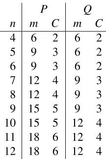
We generate two sets of instances Pand Q, such that instances of typeP allow a large number of feasible assignments (requiring an algorithm with good exploration properties), and instances of typeQallow only few feasible assignments (making ex-ploitation properties more relevant).
Both types of instances were generated in the following way. Given the number of regionsn, the number of shelters m, the number of scenarios N, and the number of shelters that can be opened C, we generate all other parameters. We uniformly randomly chooseuj ∈ {300, . . . ,800}, Di ∈ {100, . . . ,400}, andki ∈ {1, . . . ,5}for all iand j. We then distribute the number of people Di of region irandomly over theki
zones within this region. For each scenario, we then further generated by randomly distributing the number of people within each zone over the first 20 timesteps, such that the response profiles are different in each scenario, but the number of evacuees is the same. We check if a feasible assignment exists; if this is not the case, all parameters are generated again, until the instance becomes feasible. Finally, we choose∆randomly
from{0, . . . ,4}for each zone and scenario.
We show the parameter choice for n, m, andC in Table 1. We generated all in-stances with two and with five scenarios. For each parameter set, we generated ten instances (i.e., a total of 340 instances). In the following, we denote by Pn orQn the
sets of instances withnregions.
P Q
n m C m C
4 6 2 6 2
5 9 3 6 2
6 9 3 6 2
7 12 4 9 3
8 12 4 9 3
9 15 5 9 3
10 15 5 12 4
11 18 6 12 4
[image:13.612.237.345.106.268.2]12 18 6 12 4
Table 1: Instance parameters.
allow at most half of the total timelimit to be devoted to solving the evaluation prob-lem. For better comparability, the MIPEmphasis Cplex parameter is chosen so that lower bounds are neglected and more computation time is spent on finding feasible so-lutions. For our Tabu search, only the initial assignment is found using a MIP solver; all evaluations are then carried out using our heuristic algorithm. Each algorithm was given a timelimit of 10 minutes.
Additionally, we used the MIP solver with an emphasis on lower bounds and a computation time of 60 minutes for all instances to find strong lower bounds. Because some lower bounds were equal to zero, we normalized all objective values with an offset such that the lower bound is always equal to 100.
All experiments were conducted on a computer with a 16-core Intel Xeon E5-2670 processor, running at 2.60 GHz with 20MB cache, using one core per algorithm. To solve MIPs, CPLEX v.12.6 ([IBM13]) was used. The Tabu search was run five times for every instance to account for its randomness.
6.2. Results
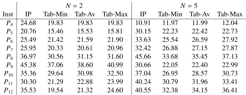
We present the average gaps over the ten instances of each size in Table 2 for the P instances, and in Table 3 for the Q instances. The gap is computed as (U B−
LB)/U B, whereU Bdenotes the respective objective value, and LBthe lower bound. In column “IP”, we show the gap when using Cplex, and show the gap for our Tabu search algorithm in columns “Tab-Min” (the average gap of the best results over the five runs per instance), “Tab-Av” (the average gap over all runs), and “Tab-Max” (the average gap of the worst result of the five runs). All values are in percent.
For allPinstances, except forP4 withN = 5, even Tab-Max considerably
N =2 N = 5
Inst IP Tab-Min Tab-Av Tab-Max IP Tab-Min Tab-Av Tab-Max
P4 24.68 19.83 19.83 19.83 10.91 11.97 11.99 12.04
P5 20.76 15.46 15.53 15.81 30.15 22.23 22.42 22.73
P6 25.49 21.42 21.59 21.90 33.63 25.54 26.59 27.92
P7 25.95 20.33 20.61 20.96 32.42 26.88 27.15 27.87
P8 36.97 30.56 31.15 31.60 45.66 33.68 35.45 37.13
P9 45.38 37.06 38.60 40.99 30.66 22.05 22.40 22.99
P10 35.36 29.64 30.98 32.50 37.04 26.95 28.57 30.73
P11 30.30 21.29 22.88 23.99 40.24 30.79 31.96 33.41
[image:14.612.88.507.162.325.2]P12 35.53 19.54 21.32 24.60 40.55 32.38 34.15 36.41
Table 2: Average gap forPinstances.
N =2 N = 5
Inst IP Tab-Min Tab-Av Tab-Max IP Tab-Min Tab-Av Tab-Max
Q4 24.68 19.83 19.83 19.83 10.91 11.97 11.99 12.04
Q5 23.16 19.55 20.11 21.00 29.45 31.16 31.23 31.38
Q6 37.45 36.48 36.64 37.02 25.38 24.23 24.75 25.02
Q7 38.96 32.91 33.77 34.87 41.58 40.08 40.52 40.72
Q8 40.72 36.77 37.46 37.94 47.86 43.70 46.09 46.90
Q9 37.58 35.67 36.34 37.07 52.62 49.96 50.73 51.48
Q10 41.52 40.46 41.10 41.76 41.20 35.80 37.06 38.34
Q11 48.38 45.17 46.14 46.79 43.24 42.73 43.57 44.36
Q12 52.35 51.15 52.39 53.05 50.66 49.65 50.83 52.21
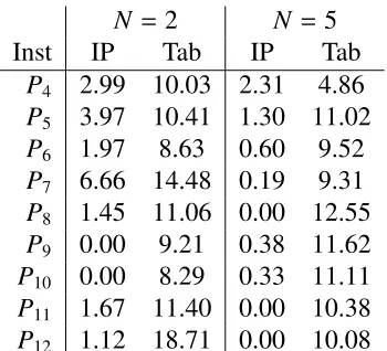
[image:14.612.87.510.480.637.2]To understand these results in more depth, we show the average difference in ob-jective gap between the starting solution and the final solution of each algorithm in Tables 4 and 5.
N = 2 N = 5
Inst IP Tab IP Tab
P4 2.99 10.03 2.31 4.86
P5 3.97 10.41 1.30 11.02
P6 1.97 8.63 0.60 9.52
P7 6.66 14.48 0.19 9.31
P8 1.45 11.06 0.00 12.55
P9 0.00 9.21 0.38 11.62
P10 0.00 8.29 0.33 11.11
P11 1.67 11.40 0.00 10.38
P12 1.12 18.71 0.00 10.08 Table 4: Average difference of gap between starting solution and final solution for P in-stances.
N =2 N = 5
Inst IP Tab IP Tab
Q4 2.99 10.03 2.31 4.86
Q5 0.16 6.19 0.48 0.23
Q6 0.00 3.30 0.00 3.36
Q7 0.34 7.03 0.00 3.06
Q8 0.05 5.62 0.00 3.72
Q9 0.00 3.76 0.00 2.66
Q10 1.30 3.76 0.00 6.23
Q11 0.00 3.94 0.00 3.21
Q12 0.00 2.92 0.00 2.43 Table 5: Average difference of gap between starting solution and final solution for Q in-stances.
We see that both the MIP solver and the Tabu search are less able to improve their respective starting solutions for instances of typeQthan for instances of typeP. Also, the Tabu search is able to improve upon its starting solution considerably more than the MIP solver; in fact, the MIP solver does not improve the starting solution at all in the vast majority of cases. This means that the gaps for IP shown in Table 3 forN =5 are due to a good exploitation of the starting solution, without any exploration at all.
6.3. Kulmbach Instance
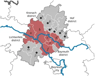
We now apply our model and algorithms to realistic data based on the Kulmbach district in north Bavaria, Germany. A map of the region can be seen in Figure 3, with keys to placenames in Tables 6 and 7. Within the Kulmbach district, the Red and White Main rivers flow together to become the Main river, and within the recent past, the region was troubled by river floodings.
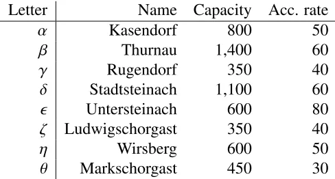
We assume that some of the people based in the subdistricts colored in red (Latin letters) need to leave their homes and make way for a shelter based in one of the other subdistricts (Greek letters). The numbers of evacuees and the numbers of zones within each region are shown in Table 6; the shelter capacity (which is based on the number of inhabitants within the region) and their accommodation rate are shown in Table 7. Of the eight shelters, six may be used.
[image:15.612.319.489.175.335.2]Kronach district
Lichtenfels district
Hof district
Bayreuth district
[image:16.612.105.479.139.447.2]Bayreuth city
Figure 3: Kulmbach district1
Letter Name Population Evacuees Zones
a Mainleus 6,449 800 3
b Kulmbach (city) 25,985 1,000 4
c K¨odnitz 1,583 250 2
d Neuenmarkt 3,040 400 1
e Trebgast 1,603 350 1
f Neudrossenfeld 3,807 700 3
g Himmelkron 3,490 600 2
Letter Name Capacity Acc. rate
α Kasendorf 800 50
β Thurnau 1,400 60
γ Rugendorf 350 40
δ Stadtsteinach 1,100 60
Untersteinach 600 80
ζ Ludwigschorgast 350 40
η Wirsberg 600 50
[image:17.612.169.413.108.239.2]θ Markschorgast 450 30
Table 7: Sheltering regions of Kulmbach district
We generate three scenarios, which correspond to different levels of evacuation urgency: In the first scenario, profilesdare chosen such that evacuees leave early and
∆is small; in the second scenario, evacuees leave late and∆is larger; the third scenario is between those two.
Both the IP model with Cplex and our Tabu search algorithm find the same solution within one minute of computation time, which can be shown to be optimal by running a subsequent IP with increased timelimit (as in the previous experiments).
The objective value of this solution is 49, which is reached in the first scenario (the objective values for the other scenarios are 11 and 14, respectively). Regionais assigned to shelterα, regionscand f are assigned to shelterβ, regionb to shelterδ, regiongto shelter, regioneto shelterζ, and regiondto shelterη.
7. Conclusion and Extensions
In this paper we considered the problem of coordinating the evacuation of several regions due to river flooding. We developed a model that includes for the first time several unique features of such an evacuation: The timing of evacuation orders with departure profiles is taken into account, as well as the choosing a set of shelters such that all evacuees can be accommodated without delays or traffic jams. By including several scenarios for different flooding outcomes, we take forecasting uncertainty into account via a robust optimization model.
This model decomposes into two subproblems: Assigning regions to shelters, and determining departure times for each zone. We developed a Tabu search heuristic that aims at conciliating exploration and exploitation in the interplay between these two problem levels. Our computation results show that we considerably outperform a MIP solver in terms of exploration, even if it is provided with a strong starting solution.
We now discuss possible extensions.
in-clude different driving times from regions to shelters: To this end, we can equivalently assume values for∆that depend on the assignment variablesz, which in turn can be linearized in the objective function, asxis a binary variable.
Additionally to the target evacuation time ∆for each zonek in any regionithere might also be a clearance time ρik specifying the point in time when evacuees from
zone k in region i can return to their homes safely. Then, an evacuation plan must include not only a time for the zones to evacuate but also a time at which the evacuees from a zone who are already at a shelter receive theclear order to return home. As evacuees usually want to be back home as soon as possible we assume no delay for this but propose an immediate response., i.e. allDik evacuees actually leave at the issued
time. One essential change by this additional option is that the shelters can be utilized more efficiently: returning evacuees can vacate spaces for new arrivals, i.e. the total capacity has to be respected individually at all times.
We model this in the IP-formulation of Section 2.2 by including the following sets of constraints:
X
t
rikt = 1 for alli∈ I,k∈ Ki (47)
X
τ<ρik
rikτ =0 for alli∈ I,k∈ Ki (48)
X
τ≤t−tk xikτ≥
X
τ≤tk
rikτ =0 for all j∈ S,t ∈ T (49)
rikt ∈B for alli∈ I,k∈ Ki,t∈ T. (50)
The capacity constraints (6) are replaced by
X
τ≤t
X
i
X
k
yikτj−rikτdik
≤uj for all j∈ S,t∈ T. (6’)
The binary variablerikt indicates the clearance order:
rikt =
1, if the evacuees from zonekin regionireceive clearance order at timet, 0, else.
Each zonekreceives exactly one clear order (47). The times of the orders is valid as it is, on the one hand, determined not before the given earliest clearance time ρik
(48) and, on the other, not before all evacuees from the zone have actually arrived at the shelter (49). (Note, that we view ρik as a hard constraint. In contrast, target
time ∆ik is a soft bound and can be violated in turn for an increase in the objective
References
[ABV09] H. Aissi, C. Bazgan, and D. Vanderpooten. Minmax and minmax regret versions of combinatorial optimization problems: A survey. European Journal of Operational Research, 197(2):427 – 438, 2009.
[AG06] N. Altay and W.G. Green III. OR/MS research in disaster operations man-agement. European Journal of Operational Research, 175(1):475 – 493, 2006.
[BTGN09] A. Ben-Tal, L. El Ghaoui, and A. Nemirovski. Robust Optimization. Princeton University Press, Princeton and Oxford, 2009.
[CTC07] M.-S. Chang, Y.-L. Tseng, and J.-W. Chen. A scenario planning approach for the flood emergency logistics preparation problem under uncertainty.
Transportation Research Part E: Logistics and Transportation Review, 43(6):737 – 754, 2007. Challenges of Emergency Logistics Management.
[GDT15] M. Goerigk, K. Deghdak, and V. TKindt. A two-stage robustness ap-proach to evacuation planning with buses. Transportation Research Part B: Methodological, 78:66 – 82, 2015.
[GG14] M. Goerigk and B. Gr¨un. A robust bus evacuation model with delayed scenario information. OR Spectrum, 36(4):923–948, 2014.
[GJ79] M.R. Garey and D.S. Johnson. Computers and intractability: a guide to NP-completeness, 1979.
[GS15] M. Goerigk and A. Sch¨obel. Algorithm engineering in robust optimiza-tion. In L. Kliemann and P. Sanders, editors,Algorithm Engineering: Se-lected Results and Surveys, volume 9220 of Lecture Notes in Computer Science, page 0. Springer Berlin/Heidelberg, 2015.
[HHH11] O. Huibregtse, A. Hegyi, and S. Hoogendoorn. Robust optimization of evacuation instructions, applied to capacity, hazard pattern, demand, and compliance uncertainty. In Networking, Sensing and Control (ICNSC), 2011 IEEE International Conference on, pages 335–340, April 2011.
[HHPB10] O. L. Huibregtse, S. P. Hoogendoorn, A. J. Pel, and M. C. J. Bliemer. A generic method to optimize instructions for the control of evacuations. In
12th IFAC symposium on transportation systems, Redondo Beach, Sept. 2009. IFAC, 2010.
[IBM13] IBM. IBM ILOG CPLEX 12.6 User’s Manual, 2013.
[JHSF+14] B. Jongman, S. Hochrainer-Stigler, L. Feyen, J.C.J.H. Aerts, R. Mechler, W.J.W. Botzen, L.M. Bouwer, G. Pflug, R. Rojas, and P.J. Ward. Increas-ing stress on disaster-risk finance due to large floods. Nature Climate Change, 4(4):264–268, 2014.
[KWLY11] A. Kulshrestha, D. Wu, Y. Lou, and Y. Yin. Robust shelter locations for evacuation planning with demand uncertainty. Journal of Transportation Safety&Security, 3(4):272–288, 2011.
[KY97] P. Kouvelis and G. Yu.Robust Discrete Optimization and Its Applications. Kluwer Academic Publishers, 1997.
[KYC05] S. Kongsomsaksakul, C. Yang, and A. Chen. Shelter location-allocation model for flood evacuation planning. Journal of the Eastern Asia Society for Transportation Studies, 6:4237–4252, 2005.
[Re13] Munich Re. Munich reinsurance company geo risks research. NatCat-SERVICE Database, 2013.