in Industrial Wireless Sensor Networks
Muhammad Farooq-I-Azam, Qiang Ni,
Senior Member, IEEE,
and Ejaz A. Ansari
Abstract—In many applications of industrial wireless sensor networks, sensor nodes need to determine their own geographic position coordinates so that the collected data can be ascribed to the location from where it was gathered. We propose a novel intelligent localization algorithm which uses variable range beacon signals generated by varying the transmission power of beacon nodes. The algorithm does not use any additional hardware resources for ranging and estimates position using only radio connectivity by passively listening to the beacon signals. The algorithm is distributed, so each sensor node determines its own position and communication overhead is avoided. As the beacon nodes do not always transmit at maximum power and no transmission power is used by unknown sensor nodes for localization, the proposed algorithm is energy efficient. It also provides control over localization granularity. Simulation results show that the algorithm provides good accuracy under varying radio conditions.
Index Terms—Localization; wireless sensor networks; multilateration; energy efficiency; location intelligence.
I. INTRODUCTION
I
N many applications of industrial wireless sensor networks, sensor nodes need to determine their own geographic positions. Examples of such industrial applications include gas leakage detection, industrial IoT, industrial fire detection, underground pipeline inspection, target tracking, habitat monitoring and area surveillance [1]–[3]. In such cases, unknown sensor nodes need to employ an intelligent localization algorithm to estimate their geographic position coordinates usually with the assistance of a few beacon nodes. The beacon nodes know their positions a priori either because these are placed at pre-determined locations or are equipped with location finding device, such as, global positioning system (GPS) receiver. Due to energy and size limitations, all unknown sensor nodes cannot be equipped with such extra piece of hardware.Location information of industrial sensor nodes is important because of two major reasons. First, the sensor nodes must send their geographic position coordinates with the sensed data because data alone without location information may not be useful. For example, in the case of an industrial fire detection application, the sensor node should send the geographic coordinates along with the event information so that location of fire is known. Second, there are many services and protocols that use location information to work. For example, certain routing protocols, [4], [5], sensing coverage [6], [7], topology management [8] and clustering strategies [9] depend upon location information of sensor nodes.
M. Farooq-i-Azam is with Lancaster University, UK and COMSATS IIT, Pakistan (email: [email protected]).
Q. Ni is with School of Computing and Communications, Lancaster University, UK (email: [email protected]).
E. A. Ansari is with Department of Electrical Engineering, COMSATS IIT, Pakistan (email: [email protected]).
Localization algorithms may be classified as range based [10] or range free [11]–[14], anchor based [10]–[12] or anchor free [15] and single hop [14] versus multihop [16]. Localization algorithm may be designed for outdoor unconstrained [11]–[17] or indoor constrained environment [18]. Similarly, a localization algorithm may use central [19] or distributed processing [11]–[14]. In localization with mobile anchor using trilateration (LMAT) [20], a moving beacon node is used to help unknown nodes estimate their positions. A single beacon node moves in a zig zag fashion along a trajectory following the shape of interconnected equilateral triangles in the sensor field to help localize unknown nodes. In the Centroid algorithm [21], an unknown sensor node determines its connectivity with neighbor beacon nodes and estimates its position at their centroid. In concentric anchor beacon (CAB) localization scheme [13], beacon nodes use two transmission levels. An unknown node chooses three most distant beacon nodes by calculating the areas of triangles of all possible combinations. Next, it calculates points of intersection of annular rings around these beacons by selecting two beacon nodes at a time. It then isolates valid points of intersection which are points that fall within all the annular rings. The unknown node localizes itself at the centroid of the region bounded by the points of intersection. Convex position estimation (CPE) [19] algorithm formulates localization as an optimization problem and then uses linear programming for position estimation.
In this paper, we present a localization algorithm which is distributed so that each unknown node can localize itself passively by just listening to beacon nodes. The algorithm employs multiple power levels [11]–[13] and annular rings around beacon nodes and uses multilateration in sensor nodes to achieve a novel but simple localization technique. The algorithm is intelligent in two aspects. First, the proposed algorithm enables a node to estimate position in an intelligent manner by using passive information from beacon nodes. Second, it provides sensing intelligence to the sensor network. For example, after estimating positions, the nodes can make many intelligent decisions, such as routing based on location information. The algorithm does not require any extra piece of hardware to estimate range and position. Based on the fact that the algorithm sends out a ripple of beacon signals, we call it ripple localization algorithm (RLA) for convenience of reference. We also show quantitatively that the algorithm is energy efficient compared to localization techniques which transmit beacon signals at fixed radio range. Approximately 92% of the upper limit of energy efficiency can be attained by using 10 quantization levels of transmission power.
This paper makes four major contributions. First, we present a novel, intelligent, distributed and energy efficient localization algorithm which gives good localization accuracy. Second, we give a quantitative analysis of energy efficiency of the
proposed algorithm. Third, we implement and simulate our intelligent localization algorithm with practical irregular radio conditions. Our localization algorithm is also compared with two related algorithms – Centroid [21] and CAB [13]. Fourth, we introduce three new metrics, error momentum, degree of location intelligence (DOLI) and localization efficiency, for the evaluation of localization algorithms. Simulation results demonstrate that our proposed localization algorithm achieves localization error which is much lower than both Centroid and CAB. Time complexity of our ripple localization algorithm is much lower than that of CAB and only marginally higher than that of Centroid.
II. RIPPLELOCALIZATIONALGORITHM
In this section, we start with assumptions of the sensor field and then describe the ripple localization algorithm. The algorithm consists of two parts – one part is executed by beacon nodes and the other by the unknown nodes.
A. Sensor Field
We consider an outdoor wireless sensor network in a two dimensional unconstrained sensor field with finite geographic boundaries in which the sensor and beacon nodes are deployed. Radio range of unknown nodes is longer compared to their sensing range so that sensing granularity of nodes is higher and sensed data can be transmitted to longer distances. Communication range of beacon nodes is longer than that of unknown sensor nodes. As a result, the beacon signal reaches a large number of unknown sensor nodes at greater distances and a fewer number of beacon nodes are required to localize a large number of unknown sensor nodes. We assume that all nodes are equipped with omnidirectional antennas, designed for sensor networks such as the one described in [22], so that nodes communicate equally in all directions. We also assume that orthogonality of beacon signals is handled by a medium access control protocol. To discuss and explain the algorithm, we assume a perfectly circular radio range. However, for performance evaluation and simulation, we use a more practical irregular radio model [14] as shown in Fig. 1. Degree of irregularity (DOI) is used to denote the extent of irregularity in radio pattern and is defined as the maximum radio range variation per unit degree change in the direction of propagation.
[image:2.612.377.496.468.615.2](a) DOI = 0 (b) DOI = 0.1 (c) DOI = 0.2 Fig. 1. Irregular radio pattern and degree of irregularity.
B. Algorithm for Beacon Nodes
In majority wireless networks, beacon nodes transmit multiple beacon signals at regular intervals using the same transmission power. As a result, all of these beacon signals have the same fixed transmission radius. In ripple localization algorithm, a beacon node transmits beacon signals at different power levels corresponding to different transmission radii so that these radii fall into certain pre-determined quantized intervals1. The beacon nodes are tested and calibrated so that transmission radii corresponding to different power levels are recorded for embedding in beacon messages. Hence, unknown nodes receive more information each time they receive a beacon message. The unknown nodes use this information to achieve better accuracy in location estimation.
Transmission of successive beacon signals with incremental values of transmission power and hence different transmission radii is shown in Fig. 2. This is analogous to a ripple in water. It emanates from the center and travels outwards. In the same manner, each beacon node generates a ripple of beacon signals. A beacon node sends its first beacon signal with some set minimum transmission power. For each successive beacon signal it increments the transmission power in such manner that the transmission radius of the beacon signal is longer by a step dr from the previous beacon signal. Beacon node increments transmission power with each successive beacon signal until maximum transmission power is reached, at which point, the beacon node resets and starts this process all over again. A typical beacon message is shown in Fig. 3. In this beacon message,t0is the time stamp.(Xb, Yb)are the position coordinates of the beacon node. Pti is the transmission power used. Ri is the corresponding radio range. dr is the beacon signal step.Rmin is the minimum transmission radius
1 2 3 4 5
P min
P max
d r
Beacon Node Unknown Node U
1 U
2
U 3 R
min R
max
U 4
[image:2.612.60.278.645.732.2]Fig. 2. A ripple of beacon signals.
Fig. 3. A typical beacon message.
corresponding to the minimum transmission power Pmin.
Rmax is the maximum transmission radius corresponding to the maximum transmission power Pmax.
Algorithm 1 Algorithm for beacon nodes
1: while(true)do
2: transmit power = minimum transmit power
3: while(transmit power≤maximum transmit power)do 4: prepare beacon message
5: transmit beacon message 6: increment transmit power 7: end while
8: end while
C. Algorithm for Unknown Nodes
Multiple unknown nodes lying within the communication range of a beacon node receive its beacon signals as shown in Fig. 2. By extracting information from all the beacon messages that an unknown node receives from a particular beacon node, it can determine the radii of the inner and outer circles of the annular ring around the beacon node in which it lies. For example, the first beacon signal that unknown node U1 receives is beacon signal number 4. Therefore, it can ascertain that outer radius of the annular ring in which it lies is the same as that of beacon signal 4. Note that, of all the beacon messages that unknown node U1 receives from that particular beacon node, first beacon signal has the smallest radius. Knowing the beacon signal step dr from the beacon message, and by subtracting it from the radius of the outer circle, it can also determine the radius of the inner circle. Next, it estimates its distance from the beacon node by calculating average of the radii of the inner and outer circles around the beacon node. Having estimated its distances from three or more neighbor beacon nodes, the unknown node then constructs and solves a set of multilateration equations to estimate its own position.
To further explain position estimation, consider an unknown sensor node having k neighbor beacon nodes with position coordinates(x1, y1),(x2, y2), ...,(xk, yk). The unknown node gets current transmission radius Ri and beacon signal step
dr of a neighbor beacon node from the beacon message and estimates its range ri from the beacon node as under:
ri=
Ri+Ri−1
2 (1)
whereRi−1 is calculated as below:
Ri−1=Ri−dr (2)
Ri and Ri−1 are radii of the outer and inner circles of the annular ring around the beacon node in which the unknown node lies. Using position coordinates of beacon nodes as centers and range estimates as calculated above as radii, a set of following equations of circles around beacon nodes can be obtained:
(x−x1)2+ (y−y1)2 (x−x2)2+ (y−y2)2
.. .
(x−xk)2+ (y−yk)2 = r2 1 r2 2 .. . r2 k (3)
Expanding square terms on the left side and rearranging, we get:
x2+y2−2x
1x−2y1y
x2+y2−2x
2x−2y2y ..
.
x2+y2−2xkx−2yky = r2
1−x21−y12
r2
2−x22−y22 .. .
r2k−x2k−y2k
(4)
Subtracting last row from each of the rows above it:
2(xk−x1)x+ 2(yk−y1)y 2(xk−x2)x+ 2(yk−y2)y
.. .
2(xk−xk−1)x+ 2(yk−yk−1)y = r2
1−rk2+x2k−x21+y2k−y21
r2
2−rk2+x2k−x22+y2k−y22 ..
.
r2k−1−rk2+x2k−x2k−1+y2k−y2k−1
(5)
Separating the unknowns(x, y), this can be rewritten in matrix form as below:
(xk−x1) (yk−y1) (xk−x2) (yk−y2)
..
. ...
(xk−xk−1) (yk−yk−1) x y = 1 2 r2
1−r2k+x2k−x21+y2k−y21
r2
2−r2k+x2k−x22+y2k−y22 ..
.
rk−2 1−r2k+x2k−x2k−1+y2k−y2k−1
(6)
Using matrix notation, this can be written as:
Az=R (7)
wherez=
x yT and A=
(xk−x1) (yk−y1) (xk−x2) (yk−y2)
..
. ...
(xk−xk−1) (yk−yk−1) (8)
R=1 2 r2
1−rk2+x2k−x21+yk2−y12
r2
2−rk2+x2k−x22+yk2−y22 ..
.
r2k−1−r2k+x2k−x2k−1+yk2−yk−2 1
(9)
Using least squares approximation, we get the following closed-form and unique solution to (7).
z=A+R (10)
where
A+= (ATA)−1AT (11)
Algorithm 2 Algorithm for unknown nodes
1: /* Step 1 */
2: construct a list of neighbor beacon nodes 3: /* Step 2 */
4: for allneighbor beacon nodesdo
5: sort beacon signal radii of received signals 6: signal with smallest radius is the outer circle
7: radius of inner circle = radius of outer circle – signal step
8: estimated range = average of radii of inner and outer circles
9: end for 10: /* Step 3 */
11: ifnumber of neighbor beacon nodes ≥3then
12: estimated position = multilaterate using all neighbor beacon nodes
13: end if
D. Proof of Concept
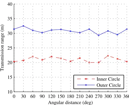
To give a proof of the basic concept used in ripple localization algorithm, we perform a simple experiment which can be easily replicated. We use a D-Link DIR-605 IEEE 802.11 wireless router operating at 2.4 GHz and a Huawei Ascend Y300 Android smartphone for our experiment. The wireless router allows its transmission power to be set at different levels through its administrative interface and is equipped with omnidirectional antennas. The WiFi Analyzer application is downloaded and installed on the smartphone from the Google Play Store. We place the wireless router in the center of a large and unobstructed open field. The power is supplied by an uninterrupted power source. Using the administrative interface, we set the transmission power of the wireless router to 15% which is the minimum level it allows. The smartphone is moved away from the wireless router until the WiFi Analyzer on the smartphone reads -95 dBm. This is the threshold power for which the smartphone provides connectivity. Further decrease in RSS results in loss of connectivity. The distance between the router and the smartphone is recorded. We repeat the same experiment every 30o making a total of 12 recordings circling 360o around the wireless router. We then set the transmission power of the wireless router to 35% which is the next level that it allows. We repeat the experiment described above and take another set of 12 readings each30oapart. We plot both sets of data in Fig. 4. The first set of data gives the inner circle corresponding to 15% transmission power whilst the second set of data constitutes the outer circle corresponding to 35% transmission power. It can be seen that the radio coverage is nearly circular. It is also evident that practical irregularity in radio is comparable to DOI used in our simulation experiments.
In the second part of our experiment, we download and install the WiFi Alarm application on the smartphone and set an alarm to sound when the WiFi network provided by the wireless router is detected. We place the smartphone in the area bounded by the transmission circles corresponding to 15% and 35% power levels. We first set the transmission power
0 30 60 90 120 150 180 210 240 270 300 330 360 10
15 20 25 30 35 40
Angular distance (deg)
Transmission range (m)
[image:4.612.331.542.59.231.2]Inner Circle Outer Circle
Fig. 4. Experimental verification of radio connectivity.
to 15%. As the smartphone is not within range, the alarm does not sound. Next, we set the transmission power to 35%. The smartphone receives and detects the wireless signal and sounds the alarm. This is repeated by placing the smartphone at 10 different positions in the annular region bounded by the two transmission circles. The alarm did not sound only once when the smartphone was placed at the outer periphery of the annular region. Experiment verifies the basic concept used in the ripple localization algorithm.
III. ENERGYEFFICIENCY
We give a quantitative analysis of the energy efficiency of the proposed ripple localization algorithm in this section. We show that a beacon node achieves 92% of the upper limit of energy efficiency with 10 quantization levels of transmission power. The unknown sensor node expends zero transmission energy for localization.
We assume that the relationship between transmitted power
Ptand received power Pr between two nodes in the outdoor unconstrained sensor field is governed by the following path loss model:
Pt
Pr
=Kdα (12)
where
K= 1
GtGr (4π
λ)
2 (13)
Gt and Gr are gains of transmitter and receiver antennas respectively, λ is the wavelength of radio waves, d is the distance between transmitter and receiver antennas, and α is the path loss exponent.
beacon signal step and denote it bydr. Furthermore, let us also assume that beacon signal minimum radio rangeRminis equal to beacon signal step dr for simplicity. Let the transmitted power of an ith beacon signal be denoted by Pti and the corresponding radio range of the beacon signal beRi. As the difference between the radii of two consecutive beacon signals
dr is constant, therefore
Ri=i×dr (14) If the total number of beacon signals in the ripple generated by the beacon node is n, then
Rmax=n×dr (15) According to (12), transmitted powerPtiforith beacon signal is given as:
Pti
Pr
=KRαi (16)
Similarly, maximum transmitted power Pmax is given by
Pmax
Pr
=KRαmax (17)
Received power Pr is the same in (16) and (17). Substituting (14) in (16) and (15) in (17), we get:
Pti
Pr
=K(idr)α (18)
Pmax
Pr
=K(ndr)α (19)
Dividing (18) by (19), we get:
Pti= (
i n)
α
Pmax (20) The above relation gives us the transmission power required to transmitith beacon signal with radiusRiin a ripple. To get the upper bound on the energy saved, we use α= 2. Therefore, total power PT transmitted by a beacon node for sending a ripple ofn beacon signals is given by:
PT =
Pmax
n2 n X
i=1
i2 (21)
Summation term on the right is the sum of squares of first n
natural numbers, which is given by:
n X
i=1
i2=n(n+ 1)(2n+ 1)
6 (22)
Substituting this in (21), we get
PT =
(n+ 1)(2n+ 1)
6n Pmax (23)
If a beacon node transmits 5 beacon messages, all at maximum power, transmit power used is 5Pmax. However, if a ripple of 5 beacon messages is transmitted by varying the transmit power, so thatn = 5, the total transmitted power, as calculated using (23) is 2.2Pmax, which is less than half of the power required to transmit usual beacon messages at maximum power. Power2 saved is 5Pmax – 2.2Pmax = 2.8Pmax and energy efficiency 2Time required to transmit beacon signals in both cases is the same. Therefore, power implies energy and vice versa.
of100×2.8/5 = 56%is achieved. In general, transmit power savedPS in transmitting a ripple ofn beacon signals is given by:
PS =nPmax−
(n+ 1)(2n+ 1)
6n Pmax (24)
This can be simplified to arrive at the following result:
PS =
(4n+ 1)(n−1)
6n Pmax (25)
This gives us the energy saved when a ripple of beacon messages is sent instead of sending beacon signals at fixed radio range. If n beacon messages are transmitted at fixed power, the transmitted power used is nPmax. Percentage of power saved or energy efficiencyηP achieved is given by:
ηP =
PS
nPmax
×100 = (4n+ 1)(n−1)
6n2 ×100 (26)
Note that forn= 1, i.e. beacon messages with only one power level, (25) and (26) result in zero implying that no energy is saved. Forn = 5,ηP is 56% which is the same as calculated earlier using (23). A plot of (26) for the interval0≤n≤10is shown in Fig. 5. As can be seen, greater the number of beacon signals n, greater is the energy saved. In the limit, when a beacon node uses an infinite number of beacon signals in a ripple, maximum energy efficiency ηP max is achieved and is given by:
ηP max= lim n→∞
(4 + 1n)(1− 1 n)
6 ×100 = 66.67% (27) This shows that the upper bound on the energy saved by a beacon node is 66.67% when the number of beacon signals in a ripple approaches∞.
Using (26), we calculate that for 60% and 65% energy saving, the number of beacon signals in a ripple is approximately 8 and 30 respectively. Forn= 10 in a ripple, we get 61.50% energy saving i.e. we attain approximately 92% of the upper limit of energy efficiency.
The above calculations show the energy that is being saved by beacon nodes only. The proposed algorithm does not require an unknown node to transmit anything. It estimates the position passively by merely receiving and processing
0 2 4 6 8 10
0% 10% 20% 30% 40% 50% 60%
Number of beacon signals (n)
[image:5.612.327.545.558.725.2]Percent saving in energy
information from beacon nodes. Therefore, unknown nodes utilizezerotransmission energy for the purpose of localization. We assert that the only energy an unknown node expends for localization is the processing energy. However, note that a complete assessment of total energy consumption of a sensor node can only be made after analysis of all the related information. This includes energy spent on receiving and how duty cycling is done for the particular application for which the sensor network has been deployed. It is further added that we are concerned only with energy used by the localization algorithm and not the overall energy used by a sensor node for various other tasks.
IV. PERFORMANCEMETRICS
In this section, we describe metrics used for performance evaluation and comparison of ripple localization algorithm. We also introduce and explain three new metrics, error momentum, localization efficiency and degree of location intelligence (DOLI), for performance evaluation of localization algorithms. Localization error is the distance between actual and estimated positions. Localization error is normalized to sensor node radio range Rs for the purpose of uniform comparison of results. Localization time is the time taken by a localization algorithm for position estimation of a sensor node. To quantify the combined effect of localization time and localization error, we introduce a new metric which we call time momentum of localization error or simply error momentum. We define error momentum as the product of localization error and localization time. If localization time of 1 second results in a localization error of 1 meter, we have unit error momentum of 1 meter-second. As localization times are usually in the range of milliseconds, meter-second is a large unit for our purpose and we, therefore, use milli meter-second instead. If localization error or time is appropriately traded off, value of error momentum will be more closer to the low value.
A localization algorithm may sometimes be not able to help all the unknown nodes localize and settle down. For example, in the case of CAB, if neighbor beacon nodes do not fulfill the set of constraints laid down by the algorithm, the sensor node fails to estimate position. This node is called anunsettlednode. A node which is able to localize is called settled or location intelligent node. If number of settled nodes is represented by
Nsand number of total unknown nodes byNu, we can define localization efficiency ηl as following:
ηl=
Ns
Nu
×100 (28)
A sensor node which does not know its position is a dumb node or unknown node. When it has estimated its position with the help of a localization algorithm, it has acquired
location intelligence. Degree of location intelligence (DOLI) of a sensor node depends upon the extent of accuracy with which it has estimated its position. An unknown or dumb node which does not know its position has a DOLI of 0. A node which knows its exact position with zero estimation error has
a DOLI of 1. We represent DOLI using Greek symbolδ and formally define it as:
δ= (
0, if el
Rs ≥Rs
Rs−Rsel
Rs , otherwise
(29)
whereRsis the radio range andelis the localization error of the unknown sensor node. If an unknown node has normalized localization error greater than or equal to its radio range,δ= 0 for such cases and for all other cases0≤δ≤1.
V. PERFORMANCEEVALUATION
We begin this section with a description of simulation settings. We then present, describe and analyze results of experiments carried out for the performance evaluation of the ripple localization algorithm (RLA) and its comparison with two other algorithms – Centroid [21] and CAB [13]. Both Centroid and CAB are designed for unconstrained environment and are closely related to our work.
A square sensor field of size 100 m×100 m with 100 randomly deployed sensor nodes is used for the simulation experiments. Transmission power of beacon nodes is changed such that they have a minimum 10 m and maximum 100 m transmission radius with a beacon signal step of 10 m. As a result, the beacon nodes use 1 to 10 transmission power levels. A practical irregular radio model as depicted in Fig. 1 is used for performance evaluation. Degree of irregularity (DOI) is used to denote the extent of irregularity and noise in radio pattern and is defined as the maximum radio range variation per unit degree change in the direction of propagation. To simulate irregular radio range of a beacon node, we use a Gaussian random variable with mean (µ) equal to the current transmission radius (Ri) of the beacon node and standard deviation(σ)equal to the product of DOI and mean. In other words, µ=Ri and σ=µ×DOI. For performance evaluation and comparison, number of beacon signals in a ripple, number of beacon nodes in the sensor field and DOI of beacon signals are varied in a number of simulation experiments and results are recorded and plotted. We use a computer with Intel Core i3-3110M CPU @2.40 GHz processor and 4 GB RAM to run the simulations. We use the same platform to simulate all the compared algorithms.
A. Localization Error
0 2 4 6 8 10 0.0
0.5 1.0 1.5 2.0 2.5 3.0 3.5 4.0
Number of beacon signals in a ripple
Localization error
[image:7.612.67.283.60.231.2]DOI = 0.0 DOI = 0.1 DOI = 0.2
Fig. 6. Effect of number of beacon signals in a ripple on localization error.
2) Number of beacon nodes: Under adverse radio conditions, with DOI = 0.2, localization error is recorded while number of beacon nodes in the sensor field is varied from 3% to 30%. Results, plotted in Fig. 7, show that RLA performs better than both Centroid and CAB over the entire range of the number of beacon nodes. Better performance of RLA can be attributed to three other reasons in addition to its usage of multiple power levels. First, the only source of error in RLA is due to least squares approximation, which in turn is due to error in estimation of distances. In the case of CAB, there are two sources of error – estimation of distances in terms of concentric rings and estimation of node position at the centroid of intersected region which is only a guess. Second, RLA constructs a mathematical model and solves a set of equations for position estimation. Third, instead of making a selection, it uses all neighbor beacon nodes for localization of sensor node resulting in a better position estimate.
3) Cumulative error distribution: CDF of the localization error of the three compared algorithms is plotted in Fig. 8 for DOI = 0.1using 10% beacon nodes in the sensor field. There are at least four observations that we can make from these
0% 5% 10% 15% 20% 25% 30% 0
1 2 3 4 5 6
Number of beacon nodes
Localization error
Centroid
CAB
RLA
Fig. 7. Localization error of Centroid, CAB and RLA.
0 1 2 3 4 5 6 7
0% 20% 40% 60% 80% 100%
Localization error
Number of sensor nodes
[image:7.612.324.546.60.233.2]Centroid CAB RLA
Fig. 8. Comparison of cumulative error distribution.
plots. First, there is a large difference in the error distribution of the three algorithms. Second, the error distribution of Centroid is spread over large values. When using Centroid, almost 50% nodes have localization error between 2Rs and 4.5Rs, and remaining 50% have error between 4.5Rs and 7Rs which are quite large values. Third, CDF plot for RLA algorithm is relatively vertical compared to the other two algorithms. It means that there is comparatively smaller spread in localization error and accuracy of localization can be predicted with more certainty in the case of RLA algorithm. 100% nodes are able to localize with error below Rs and approximately 90% nodes have error below 0.75Rs using RLA algorithm. Fourth, in the case of CAB algorithm, approximately 40% nodes have localization error below Rs. All other nodes using CAB have localization error greater than Rs. Localization errors above Rs imply that the node has localized itself beyond its area of radio coverage and the estimated position may lie in the area of coverage of another sensor node.
B. Localization Time
[image:7.612.69.278.556.725.2]the other hand, RLA gives better location accuracy without any significant increase in time, as it does not need repetitive computation for position estimation. It is to be noted that, while CAB requires significantly higher amount of processing energy, it needs the same amount of transmission energy as used by RLA when transmitting beacon signals using the same number of power levels.
C. Error Momentum
In Fig. 9, the three algorithms are compared with respect to localization time, and in Fig. 7, the same algorithms are compared with respect to localization error. In terms of localization error, CAB algorithm performs better than the Centroid. However, with respect to localization time, performance of Centroid algorithm is better than CAB. We can use error momentum to determine which of the two algorithms makes better use of localization time and error trade off. In Fig. 10, we plot error momentum of the three algorithms for different values of DOI as the number of beacon nodes in the sensor field is increased. CAB performs better when the number of beacon nodes is between 5% to 23%. However, Centroid algorithm makes better use of time and error trade
0% 5% 10% 15% 20% 25% 30%
0 50 100 150 200
Number of beacon nodes
Localization time (ms)
[image:8.612.323.545.345.516.2]Centroid CAB RLA
Fig. 9. Comparison of localization times.
0%
10%
20%
30%
0.00 0.05 0.10 0.15 0.20
0 20 40 60 80
Number of beacon nodes Degree of irregularity
Error momentum
[image:8.612.64.283.349.518.2]Centroid CAB RLA
Fig. 10. Change in error momentum with DOI and number of beacon nodes.
off when the number of beacon nodes is below 5% or is greater than 23%. RLA performs better than both Centroid and CAB.
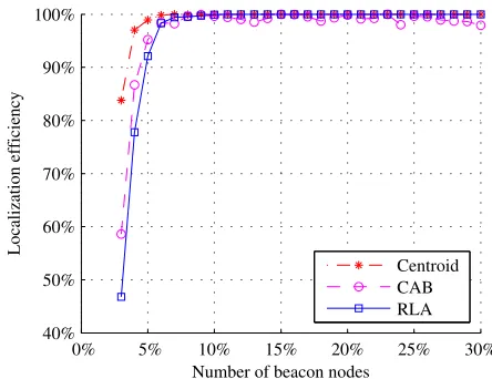
D. Localization Efficiency
In Fig. 11, we plot localization efficiency of the three compared algorithms for DOI = 0.2. Centroid and RLA algorithms achieve 100% localization efficiency when the number of beacon nodes is increased beyond 5%. CAB algorithm also achieves almost 100% efficiency beyond this point with occasional exceptions. In the case of CAB algorithm, a node has to first calculate points of intersection of transmission circles of neighbor beacon nodes and then isolate
valid points of intersection. Due to irregular radio pattern, isolation of valid points of intersection may not be possible sometimes thereby resulting in lower localization efficiency.
E. Degree of Location Intelligence
DOLI for the three algorithms is plotted in Fig. 12 for DOI = 0.2. Sensor nodes have better DOLI when using RLA compared to either Centroid or CAB for the entire range of beacon nodes. Beyond 10% beacon nodes, DOLI of RLA remains above 0.95.
0% 5% 10% 15% 20% 25% 30% 40%
50% 60% 70% 80% 90% 100%
Number of beacon nodes
Localization efficiency
Centroid CAB RLA
Fig. 11. Localization efficiency.
0% 5% 10% 15% 20% 25% 30%
0.0 0.2 0.4 0.6 0.8 1.0
Number of beacon nodes
Degree of location intelligence Centroid
[image:8.612.327.543.555.724.2]CAB RLA
[image:8.612.60.290.564.722.2]F. Node Density
In Fig. 13, we plot localization error as side of the square sensor field is increased from 50 m to 200 m while using 100 sensor nodes, 20% beacon nodes and DOI = 0.2. As the size of the sensor field increases, the beacon node density decreases. Consequently, a sensor node has fewer and distant neighbor beacon nodes, and as a result, higher distance estimation and localization error while using any of the three compared algorithm.
G. Variation in Beacon Signal Step
In a practical situation, it is possible that beacon signal step (dr) does not remain constant as the transmission power is increased successively. We add an error to the beacon signal step dr in each wave in a ripple in a 100×100 sensor field with 100 sensor nodes and 20% beacon nodes usingn= 10. The error is random over the interval[−βdr +βdr], whereβ specifies bound on the random error. We vary error bound β
from 0% to 100%, and record localization error. The results are plotted in Fig. 14. The addition of the random error in
dr may cause a sensor node to incorrectly estimate itself lying in a wrong annular ring around a neighbor beacon node, thereby yielding a faulty distance estimate, and hence, higher localization error. Transmission power of sensor node can be calibrated to minimize error in the beacon signal step.
H. Performance Comparison with Improved CAB
It may be considered to modify CAB to give improved performance. CAB can be modified in two ways. First, it can either use only three farthest beacon nodes or select all neighbor beacon nodes for position estimation. When using all neighbor beacon nodes, an unknown node does not test for the farthest three nodes. it simply selects all neighbor beacon nodes and then estimates position as in original CAB. Second, the number of transmission power levels can be kept as in CAB or increased to such levels as proposed in RLA. This gives us the following four possibilities of CAB.
50 100 150 200
0.0 0.5 1.0 1.5 2.0 2.5 3.0 3.5 4.0
Side of square sensor field (m)
Localization error
Centroid
CAB
[image:9.612.324.548.58.230.2]RLA
Fig. 13. Localization error for different sizes of sensor field.
0% 20% 40% 60% 80% 100%
0.00 0.50 1.00 1.50 2.00
Bound on random error in beacon signal step
Localization error
DOI = 0.0 DOI = 0.1 DOI = 0.2
Fig. 14. Effect of variations in beacon signal step on localization error.
1) CAB: Use the same transmission power level as in CAB and select three farthest beacon nodes for position estimation. This is original CAB algorithm.
2) CAB-A: Use a higher number of transmission levels but only three farthest beacon nodes.
3) CAB-B: While keeping the number of power levels same as in CAB, use all neighbor beacon nodes for position estimation instead of the farthest three.
4) CAB-C: With a higher number of power levels, use all neighbor beacon nodes for localization.
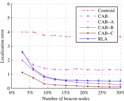
We investigate all these forms for performance comparison. We plot localization times in Fig. 15 and localization error in Fig. 16 against the number of beacon nodes for RLA and the original and the modified form of CAB using n= 10 forDOI = 0.2 with 100 sensor nodes deployed in100×100 sensor field. Accuracy of modified versions of CAB is better as localization error is lower. The two factors i.e. inclusion of all neighbor beacon nodes for position estimation and the usage of higher number of transmission levels result in smaller area bounded by points of intersection, and hence, lower localization error. However, both these factors also
0% 5% 10% 15% 20% 25% 30%
0 1000 2000 3000 4000 5000 6000
Number of beacon nodes
Localization time (ms)
[image:9.612.59.293.556.725.2]Centroid CAB CAB−A CAB−B CAB−C RLA
[image:9.612.323.545.557.724.2]0% 5% 10% 15% 20% 25% 30% 0
1 2 3 4 5 6
Number of beacon nodes
Localization error
[image:10.612.69.279.59.231.2]Centroid CAB CAB−A CAB−B CAB−C RLA
Fig. 16. Localization error of modified forms of CAB.
result in increased localization times which are plotted in Fig. 15, and lower localization efficiency which is plotted in Fig. 17. Complexity of CAB-B and CAB-C increases as the number of beacon nodes increases because a sensor node has to calculate a higher number of points of intersection and then determine valid points among them. Maximum number of points of intersection contributed by k beacon nodes is
8k(k−1)
2 = 4k(k−1)resulting in time complexity of the order ofO(k2). Each of these points of intersection is tested against
k annular rings around kbeacon nodes. Hence, total number of tests performed by an unknown node to determine valid points is4k2(k−1) giving a time complexity ofO(k3).
All modified versions of CAB are unable to localize a large number of unknown nodes, as shown in Fig. 17. Due to irregular radio, a sensor node may incorrectly determine itself lying in a different annular ring than the one it actually lies in around a beacon node. As required by CAB, a point of intersection must fall within the annular rings of all
participating neighbor beacon nodes for it to be a valid point of intersection. Due to a single incorrect annular ring, no point of intersection can satisfy this condition resulting in failure to
0% 5% 10% 15% 20% 25% 30% 0%
20% 40% 60% 80% 100%
Number of beacon nodes
Localization efficiency
Centroid
CAB
CAB−A
CAB−B CAB−C
[image:10.612.63.281.557.724.2]RLA
Fig. 17. Localization efficiency of modified forms of CAB.
isolate valid points. Therefore, node is unable to localize and remains unsettled. Ripple localization algorithm, however, has the advantage that it absorbs an incorrect annular ring during position estimation. When using Centroid or RLA, an incorrect annular ring results in a wrong range estimate, and hence it merely contributes to localization error. However, it does not block a node from localization.
VI. CONCLUSION
We have presented an intelligent, energy efficient and distributed localization algorithm for industrial wireless sensor networks. The algorithm is able to estimate position without using any additional piece of hardware thereby saving cost, size and energy. The algorithm is energy efficient. It does not require unknown nodes to expend any transmission energy and they can localize passively in an intelligent manner using only processing energy by merely listening to the beacon messages. It achieves 100% localization efficiency with a high degree of location intelligence within a short localization time by using only 5% beacon nodes. It also provides control over localization granularity.
REFERENCES
[1] K. Derr and M. Manic, “Wireless sensor networks—Node localization for various industry problems,” IEEE Trans. Ind. Informat., vol. 11, no. 3, pp. 752–762, June 2015.
[2] D. Wu, D. Chatzigeorgiou, K. Youcef-Toumi, and R. Ben-Mansour, “Node localization in robotic sensor networks for pipeline inspection,”
IEEE Trans. Ind. Informat., vol. 12, no. 2, pp. 809–819, April 2016. [3] F. Chraim, Y. B. Erol, and K. Pister, “Wireless gas leak detection and
localization,”IEEE Trans. Ind. Informat., vol. 12, no. 2, pp. 768–779, April 2016.
[4] X. Li, J. Yang, A. Nayak, and I. Stojmenovic, “Localized geographic routing to a mobile sink with guaranteed delivery in sensor networks,”
IEEE J. Sel. Areas Commun., vol. 30, no. 9, pp. 1719–1729, 2012. [5] L. Shu, Y. Zhang, L. Yang, Y. Wang, M. Hauswirth, and N. Xiong,
“TPGF: Geographic routing in wireless multimedia sensor networks,”
Telecommunication Systems, vol. 44, no. 1-2, pp. 79–95, 2010. [6] H. Mahboubi, K. Moezzi, A. Aghdam, K. Sayrafian-Pour, and
V. Marbukh, “Distributed deployment algorithms for improved coverage in a network of wireless mobile sensors,” IEEE Trans. Ind. Informat., vol. 10, no. 1, pp. 163–174, Feb 2014.
[7] C. Zhu, C. Zheng, L. Shu, and G. Han, “A survey on coverage and connectivity issues in wireless sensor networks,” Journal of Network and Computer Applications, vol. 35, no. 2, pp. 619 – 632, 2012. [8] L. LoBello and E. Toscano, “An adaptive approach to topology
management in large and dense real-time wireless sensor networks,”
IEEE Trans. Ind. Informat., vol. 5, no. 3, pp. 314–324, Aug 2009. [9] R. Xie and X. Jia, “Transmission-efficient clustering method for wireless
sensor networks using compressive sensing,” IEEE Trans. Parallel Distrib. Syst., vol. 25, no. 3, pp. 806–815, March 2014.
[10] P. Oguz-Ekim, J. Gomes, J. Xavier, M. Stosic, and P. Oliveira, “An angular approach for range-based approximate maximum likelihood source localization through convex relaxation,” IEEE Trans. Wireless Commun., vol. 13, no. 7, pp. 3951–3964, July 2014.
[11] N. Bulusu, “Self-configuring localization systems,” Ph.D. dissertation, University of California, Los Angeles, 2002.
[12] C. Liu, K. Wu, and T. He, “Sensor localization with ring overlapping based on comparison of received signal strength indicator,” in
Proceedings of IEEE International Conference on Mobile Ad-hoc and Sensor Systems, October 2004, pp. 516 – 518.
[13] V. Vivekanandan and V. W. S. Wong, “Concentric anchor beacon localization algorithm for wireless sensor networks,”IEEE Trans. Veh. Technol., vol. 56, no. 5, pp. 2733 – 2744, Sep 2007.
[14] T. He, C. Huang, B. M. Blum, J. A. Stankovic, and T. Abdelzaher, “Range-free localization schemes for large scale sensor networks,” in
[15] O.-H. Kwon, H.-J. Song, and S. Park, “Anchor-free localization through flip-error-resistant map stitching in wireless sensor network,” IEEE Trans. Parallel Distrib. Syst., vol. 21, no. 11, pp. 1644–1657, Nov 2010. [16] D. Niculescu and B. Nath, “Ad hoc positioning system (APS),” inIEEE
GLOBECOM ’01., vol. 5, 2001, pp. 2926–2931 vol.5.
[17] M. L. Sichitiu, V. Ramadurai, and P. Peddabachagari, “Simple algorithm for outdoor localization of wireless sensor networks with inaccurate range measurements,” inProceedings of International Conference on Wireless Networks, Las Vegas, 2003, pp. 300 – 305.
[18] J. M. Pak, C. K. Ahn, Y. Shmaliy, and M. T. Lim, “Improving reliability of particle filter-based localization in wireless sensor networks via hybrid particle/FIR filtering,”IEEE Trans. Ind. Informat., vol. 11, no. 5, pp. 1089–1098, Oct 2015.
[19] L. Doherty, K. pister, and L. El Ghaoui, “Convex position estimation in wireless sensor networks,” in INFOCOM 2001. Twentieth Annual Joint Conference of the IEEE Computer and Communications Societies. Proceedings. IEEE, vol. 3, 2001, pp. 1655–1663 vol.3.
[20] J. Jiang, G. Han, H. Xu, L. Shu, and M. Guizani, “LMAT: Localization with a mobile anchor node based on trilateration in wireless sensor networks,” inIEEE GLOBECOM, Dec 2011, pp. 1–6.
[21] N. Bulusu, J. Heidemann, and D. Estrin, “GPS-less low-cost outdoor localization for very small devices,” Personal Communications, IEEE, vol. 7, no. 5, pp. 28–34, Oct 2002.