Statistical Decision Making for Optimal Budget Allocation in Crowd Labeling

(1)

Statistical Decision Making for Optimal Budget Allocation

in Crowd Labeling

Xi Chen [email protected]

Stern School of Business New York University

New York, New York, 10012, USA

Qihang Lin [email protected]

Tippie College of Business University of Iowa

Iowa City, Iowa, 52242, USA

Dengyong Zhou [email protected]

Microsoft Research

Redmond, Washington, 98052, USA

Editor:Yuan (Alan) Qi

Abstract

It has become increasingly popular to obtain machine learning labels through commercial crowdsourcing services. The crowdsourcing workers or annotators are paid for each label they provide, but the task requester usually has only a limited amount of the budget. Since the data instances have different levels of labeling difficulty and the workers have different reliability for the labeling task, it is desirable to wisely allocate the budget among all the instances and workers such that the overall labeling quality is maximized. In this paper, we formulate the budget allocation problem as a Bayesian Markov decision process (MDP), which simultaneously conducts learning and decision making. The optimal allocation pol-icy can be obtained by using the dynamic programming (DP) recurrence. However, DP quickly becomes computationally intractable when the size of the problem increases. To solve this challenge, we propose a computationally efficient approximate policy which is called optimistic knowledge gradient. Our method applies to both pull crowdsourcing mar-ketplaces with homogeneous workers and push marmar-ketplaces with heterogeneous workers. It can also incorporate the contextual information of instances when they are available. The experiments on both simulated and real data show that our policy achieves a higher labeling quality than other existing policies at the same budget level.

Keywords: crowdsourcing, budget allocation, Markov decision process, dynamic pro-gramming, optimistic knowledge gradient

1. Introduction

(2)

Mechanical Turk, a much more efficient way is to post unlabeled data to a crowdsourcing marketplace, where a big crowd of low-paid workers can be hired instantaneously to perform labeling tasks.

Despite its high efficiency and immediate availability, crowd labeling raises many new challenges. Since labeling tasks are tedious and workers are usually non-experts, labels generated by the crowd suffer from low quality. As a remedy, most crowdsourcing services resort to labeling redundancy to reduce the labeling noise, which is achieved by collecting multiple labels from different workers for each data instance. In particular, a crowd labeling process can be described as a two phase procedure:

1. In the first phase, unlabeled data instances are assigned to a crowd of workers and multiple raw labels are collected for each data instance.

2. In the second phase, for each data instance, one aggregates the collected raw labels to infer its true label.

In principle, more raw labels will lead to a higher chance of recovering the true label. However, each raw label comes with a cost: the requester has to pay workers pre-specified monetary reward for each label they provide, usually, regardless of the label’s correctness. For example, a worker typically earns 10 cents by categorizing a website as porn or not. In practice, the requester has only a limited amount of budget which essentially restricts the total number of raw labels that he/she can collect. This raises a challenging question central in crowd labeling: What is the best way to allocate the budget among data instances and workers so that the overall accuracy of aggregated labels is maximized ?

The most important factors that decide how to allocate the budget are the intrinsic char-acteristics of data instances and workers: labeling difficulty/ambiguity for each data instance

andreliability/quality of each worker. In particular, an instance is less ambiguous if its label can be decided based on the common knowledge and a vast majority of reliable workers will provide the same label for it. In principle, we should avoid spending too much budget on those easy instances since excessive raw labels will not bring much additional information. In contrast, for an ambiguous instance which falls near the boundary of categories, even those reliable workers will still disagree with each other and generate inconsistent labels. For those ambiguous instances, we are facing a challenging decision problem on how much budget that we should spend on them. On one hand, it is worth to collect more labels to boost the accuracy of the aggregate label. On the other hand, since our goal is to maximize the overall labeling accuracy, when the budget is limited, we should simply put those few highly ambiguous instances aside to save budget for labeling less difficult instances. In addition to the ambiguity of data instances, the other important factor is the reliability of each worker and, undoubtedly, it is desirable to assign more instances to those reliable workers. Despite their importance in deciding how to allocate the budget, both the data ambiguity and workers’ reliability are unknown parameters at the beginning and need to be updated based on the stream of collected raw labels in an online fashion. This further suggests that the budget allocation policy should be dynamic and simultaneously conduct parameter estimation and decision making.

(3)

Process (MDP) (Puterman, 2005), whose state variables are the posterior distributions of these variables, which are updated by each new label. Here, the Bayesian setting is nec-essary. We will show that an optimal policy only exists in the Bayesian setting. Using the MDP formulation, the optimal budget allocation policy for any finite budget level can be readily obtained via the dynamic programming (DP). However, DP is computationally intractable for large-scale problems since the size of the state space grows exponentially in budget level. The existing widely-used approximate policies, such as approximate Gittins index rule (Gittins, 1989) or knowledge gradient (KG) (Gupta and Miescke, 1996; Frazier et al., 2008), either has a high computational cost or poor performance in our problem. In this paper, we propose a new policy, calledoptimistic knowledge gradient (Opt-KG). In par-ticular, the Opt-KG policy dynamically chooses the next instance-worker pair based on the optimistic outcome of the marginal improvement on the accuracy, which is a function of state variables. We further propose a more general Opt-KG policy using the conditional value-at-risk measure (Rockafellar and Uryasev, 2002). The Opt-KG is computationally efficient, achieves superior empirical performance and has some asymptotic theoretical guarantees.

To better present the main idea of our MDP formulation and the Opt-KG policy, we start from the binary labeling task (i.e., providing the category, either positive or negative, for each instance). We first consider the pull marketplace (e.g., Amazon Mechanical Turk or Galaxy Zoo) , where the labeling requester can only post instances to the general worker pool with either anonymous or transient workers, but cannot assign to an identified worker. In a pull marketplace, workers are typically treated as homogeneous and one models the entire worker pool instead of each individual worker. We further assume that workers are fully reliable (or noiseless) such that the chance that they make an error only depend on instances’ own ambiguity. At a first glance, such an assumption may seem oversimplified. In fact, it turns out that the budget-optimal crowd labeling under such an assumption has been highly non-trivial. We formulate this problem into a Bayesian MDP and propose the computational efficient Opt-KG policy. We further prove that the Opt-KG policy in such a setting is asymptotically consistent, that is, when the budget goes to infinity, the accuracy converges to 100% almost surely.

Then, we extend the MDP formulation to deal with push marketplaces with heteroge-neousworkers. In a push marketplace (e.g., data annotation team in Microsoft Bing group), once an instance is allocated to an identified worker, the worker is required to finish the instance in a short period of time. Based on the previous model for fully reliable workers, we further introduce another set of parameters to characterize workers’ reliability. Then our decision process simultaneously selects the next instance to label and the next worker for labeling the instance according to the optimistic knowledge gradient policy. In fact, the proposed MDP framework is so flexible that we can further extend it to incorporate contextual information of instances whenever they are available (e.g., as in web search and advertising applications discussed in Li et al., 2010) and to handle multi-class labeling.

In summary, the main contribution of the paper consists of the three folds: (1) we formulate the budget allocation in crowd labeling into a MDP and characterize theoptimal

(4)

The rest of this paper is organized as follows. In Section 2, we first present the modeling of budget allocation process for binary labeling tasks with fully reliable workers and motivate our Bayesian modeling. In Section 3, we present the Bayesian MDP and the optimal policy via DP. In Section 4, we propose a computationally efficient approximate policy, Opt-KG. In Section 5, we extend our MDP to model heterogeneous workers with different reliability. In Section 6, we present other important extensions, including incorporating contextual information and multi-class labeling. In Section 7, we discuss the related works. In Section 8, we present numerical results on both simulated and real data sets, followed by conclusions in Section 9.

2. Binary Labeling with Homogeneous Noiseless Workers

We first consider the budget allocation problem in a pull marketplace with homogeneous noiseless workers for binary labeling tasks. We note that such a simplification is important for investigating this problem, since the incorporation of workers’ reliability and extensions to multiple categories become rather straightforward once this problem is correctly modeled (see Section 5 and 6).

Suppose that there are K instances and each one is associated with a latent true label

Zi ∈ {−1,1} for 1≤i ≤K. Our goal is to infer the set of positive instances, denoted by

H∗ = {i : Zi = 1}. Here, we assume that the homogeneous worker pool is fully reliable or noiseless. We note that it does not mean that each worker knows the true label Zi. Instead, it means that fully reliable workers will do their best to make judgments but their labels may be still incorrect due to the instance’s ambiguity. Further, we model thelabeling difficulty/ambiguityof each instance by a latent soft-labelθi, which can be interpreted as the percentage of workers in the homogeneous noiseless crowd who will label thei-th instance as positive. In other words, if we randomly choose a worker from a large crowd of fully reliable workers, we will receive a positive label for thei-th instance with probabilityθi and a negative label with probability 1−θi. In general, we assume the crowd is large enough so that the value of θi can be any value in [0,1]. To see how θi characterizes the labeling difficulty of the i-th instance, we consider a concrete example where a worker is asked to label a person as adult (positive) or not (negative) based on the photo of that person. If the person is more than 25 years old, most likely, the corresponding θi will be close to 1, generating positive labels consistently. On the other hand, if the person is younger than 15, she may be labeled as negative by almost all the reliable workers sinceθi is close to 0. In both of this cases, we regard the instance (person) easy to label since Zi can be inferred with a high accuracy based on only a few raw labels. On the contrary, for a person is one or two years below or above 18, theθi is near 0.5 and the numbers of positive and negative labels become relatively comparable so that the corresponding labeling task is very difficult. Given the definition of soft labels, we further make the following assumption:

Assumption 1 We assume that the soft-label θi is consistent with the true label in the

sense that Zi = 1 if and only if θi ≥ 0.5, i.e., the majority of the crowd are correct, and

hence H∗ ={i:θi ≥0.5}.

(5)

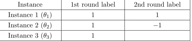
Instance 1st round label 2nd round label

Instance 1 (θ1) 1 1

Instance 2 (θ2) 1 −1

Instance 3 (θ3) 1

Table 1: Toy example with 3 instances and 5 collected labels. Instance 1 has two positive labels, instance 2 has one positive and one negative label, and instance 3 has only one positive label. The question is that, given only one more labeling chance, which instance should be chosen to label?

phase is the budget allocation phase, which is a dynamic decision process with T stages. In each stage 0 ≤ t ≤ T −1, an instance it ∈ A = {1, . . . , K} is selected based on the historical labeling results. Once it is selected, it will be labeled by a random worker from the homogeneous noiseless worker pool. According to the definition ofθit, the label received,

denoted by yit ∈ {−1,1}, will follow the Bernoulli distribution with the parameterθit:

Pr (yit = 1) =θit and Pr (yit =−1) = 1−θit. (1)

We note that, at this moment, all workers are assumed to be homogeneous and noiseless so thatyit only depends onθit but not on which worker provides the label. Therefore, it is

suffice for the decision maker (e.g., requester or crowdsourcing service) to select the instance in each stage instead of an instance-worker pair.

The second phase is the label aggregation phase. When the budget is exhausted, the decision maker needs to infer true labels {Zi}ni=1 by aggregating all the collected labels. According to Assumption 1, it is equivalent to infer the set of positive instances whose

θi ≥0.5. LetHT be the estimated positive set. The final overall accuracy is measured by

|HT ∩H∗|+|(HT)c∩(H∗)c|, the size of the mutual overlap between H∗ and HT.

Our goal is to determine the optimal allocation policy, (i0, . . . , iT−1), so that overall accuracy is maximized. Here, a natural question to ask is whether the optimal allocation policy exists and what assumptions do we need for the existence of the optimal policy. To answer this question, we provide a concrete example, which motivates our Bayesian modeling.

2.1 Why We Need a Bayesian Modeling

(6)

Current Accuracy y= 1 y=−1 Expected Accuracy Improvement

θ1>0.5 1 1 1 1 0

θ1<0.5 0 0 0 0 0

θ2>0.5 0.5 1 0 θ2 θ2−0.5>0

θ2<0.5 0.5 0 1 1−θ2 0.5−θ2 >0

θ3>0.5 1 1 0.5 θ3+ 0.5(1−θ3) 0.5(θ3−1)<0

θ3<0.5 0 0 0.5 0.5(1−θ3) 0.5(1−θ3)>0

Table 2: Expected improvements in accuracy for collecting an extra label, i.e., the expected accuracy of obtaining one more label minus the current expected accuracy. The 3rd and 4th columns contain the accuracies with the next label being 1 and −1. The 5th is the expected accuracy which is computed by takingθtimes the 3rd column plus (1−θ) times the 4th. The last column contains the expected improvements which is computed by taking the difference between the 5th and 2nd columns.

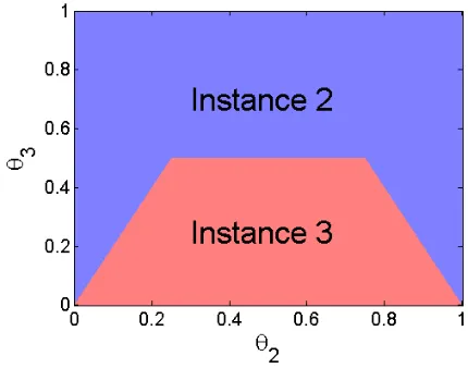
Figure 1: Decision Boundary.

Let us compute the expected improvement in accuracy in terms of the frequentist risk in Table 2. We assume that θi 6= 0.5 and if the number of 1 and −1 labels are the same for an instance, the accuracy is 0.5 based on a random guess. From Table 2, we should not label the first instance since the improvement is always 0. This coincides with our intuition. When max(θ2−0.5,0.5−θ2)>0.5(1−θ3) orθ3 >0.5, which corresponds to the blue region in Figure 1, we should choose to label the second instance. Otherwise, we should ask the label for the third one. Since the true value of θ2 and θ3 are unknown, a optimal policy does not exist under the frequentist paradigm. Further, it will be difficult to estimate θ2 and θ3 accurately when the budget is very limited.

(7)

instead of for any possible values of{θi}ni=1. Therefore, we can optimally determine the next instance to label by taking another expectation over the distribution ofθi. In this paper, we adopt the Bayesian modeling to formulate the budget allocation problem in crowd labeling.

3. Bayesian MDP and Optimal Policy

In this section, we first introduce the Bayesian MDP for modeling the dynamic budget allo-cation process and then provide the optimal alloallo-cation policy using dynamic programming.

3.1 Bayesian Modeling

We assume that each θi is drawn from a known Beta prior Beta(a0i, b0i). Beta is a rich family of distributions in the sense that it exhibits a fairly wide variety of shapes on the domain ofθi, i.e., the unit interval [0,1]. For presentation simplicity, instead of considering a full Bayesian model with hyper-priors on a0_i and b0_i, we fix a0_i and b0_i at the beginning. In practice, if the budget is sufficient, one can first label each instance equally many times to pre-estimate {a0_i, b0_i}K

i=1 before the dynamic labeling procedure is invoked. Otherwise, when there is no prior knowledge, we can simply assume a0_i = b0_i = 1 so that the prior is a uniform distribution. According to our simulated experimental results in Section 8.1.2, uniform prior works reasonably well unless the data is highly skewed in terms of class distribution. Other commonly used uninformative priors such as Jeffreys prior or reference prior (Beta(1/2,1/2)) or Haldane prior (Beta(0,0)) can also be adopted (see Robert, 2007 for more on uninformative priors). Choices of prior distributions are discussed in more details in Section 4.2.

At each stagetwith Beta(at_i, bt_i) as the current posterior distribution forθi, we make a de-cision by choosing an instanceit∈ A={1, . . . , K}and acquire its labelyit ∼Bernoulli(θit).

HereAdenotes theaction set. By the fact that Beta is the conjugate prior of the Bernoulli, the posterior of θit in the staget+ 1 will be updated as:

Beta(at_i+1_t , bt_i_t+1) = (

Beta(at_i_t+ 1, bt_i_t) if yit = 1;

Beta(at_i_t, bt_i_t + 1) if yit =−1.

We put{at_i, bt_i}K

i=1 into aK×2 matrixSt, called astate matrix, and letSit= (ati, bti) be the

i-th row ofSt. The update of the state matrix can be written in a more compact form:

St+1= (

St+ (eit,0) ifyit = 1; St+ (0,eit) ifyit =−1,

(2)

where eit is a K ×1 vector with 1 at the it-th entry and 0 at all other entries. As we

can see,{St_}_{is a Markovian process because} _St+1 _{is completely determined by the current} stateSt, the action it and the obtained labelyit. It is easy to calculate thestate transition probability Pr(yit|S

t_{, i}

t), which is the posterior probability that we are in the next state

St+1 if we chooseitto be label in the current state St:

Pr(yit = 1|S

t_{, i}

t) =E(θit|S

t_{) =} a t it

at_i_t+bt_i_t and Pr(yit =−1|S

t_{, i} t) =

bt_i_t

(8)

Given this labeling process, the budget allocation policy is defined as a sequence of decisions: π = (i0, . . . , iT−1). Here, we require decisions depend only upon the previous information. To make this more formal, we define a filtration {F_t}T

t=0, where Ft is the information collected until the staget−1. More precisely,F_tis the theσ-algebra generated by the sample path (i0, yi0, . . . , it−1, yit−1). We require the actionitis determined based on

the historical labeling results up to the staget−1, i.e.,it isFt-measurable.

3.2 Inference About True Labels

As described in Section 2, the budget allocation process has two phases: the dynamic budget allocation phase and the label aggregation phase. Since the goal of the dynamic budget allocation in the first phase is to maximize the accuracy of aggregated labels in the second phase, we first present how to infer the true label via label aggregation in the second phase. When the decision process terminates at the stageT, we need to determine a positive set

HT to maximize theconditional expected accuracy conditioning on FT, which corresponds to minimizing the posterior risk:

HT = arg max H⊂{1,...,K}

E

K

X

i=1

1(i∈H)·1(i∈H∗) +1(i6∈H)·1(i6∈H∗)

F_T !

, (4)

where 1(A) is the indicator function, which takes the value 1 if the event A is true and 0 otherwise. The term inside expectation in (4) is the binary labeling accuracy which can also be written as|H∩H∗|+|Hc_∩₍_H∗₎c_|_.

We first observe that, for 0 ≤ t ≤ T, the conditional distribution θi|Ft is exactly the posterior distribution Beta(at_i, bt_i), which depends on the historical sampling results only through S_it= (at_i, bt_i). Hence, we define

I(a, b)= Pr(. θ≥0.5|θ∼Beta(a, b)), (5)

P_it= Pr(. i∈H∗|Ft) = Pr(θi≥0.5|Ft) = Pr(θi ≥0.5|Sit) =I(ati, bti). (6)

As shown in Xie and Frazier (2013), the optimal positive setHT can be determined by the Bayes decision rule as follows.

Proposition 2 HT ={i: Pr(i∈H∗|FT)≥0.5}={i:P_iT ≥0.5} solves (4). The proof of Proposition 2 is given in the appendix for completeness.

With Proposition 2 in place, we plug the optimal positive set HT into the right hand side of (4) and the conditional expected accuracy givenFT can be simplified as:

E

K

X

i=1

1(i∈HT)·1(i∈H∗) +1(i6∈HT)·1(i6∈H∗)

FT

!

= K

X

i=1

h(P_iT), (7)

(9)

Corollary 3 I(a, b) > 0.5 if and only if a > b and I(a, b) = 0.5 if and only if a = b. Therefore, HT ={i:aiT ≥bTi } solves (4).

By viewinga0_i andb0_i as pseudo-counts of 1s and−1s at the initial stage, the parameters

aT_i andbT_i are the total counts of 1s and−1s. The estimated positive setHT ={i:aT_i ≥bT_i } consists of instances with more (or equal) counts of 1s than that of −1s. When a0_i = b0_i,

HT is constructed exactly according to the vanillamajority vote rule.

To find the optimal allocation policy which maximizes the expected accuracy, we need to solve the following optimization problem:

V(S0)= sup. π E

π

"

E

K

X

i=1

1(i∈HT)·1(i∈H∗) +1(i6∈HT)·1(i6∈H∗)

F_T !#

= sup π E

π K

X

i=1

h(P_iT) !

, (8)

where Eπ represents the expectation taken over the sample paths (i0, yi0, . . . , iT−1, yiT−1)

generated by a policy π. The second equality is due to Proposition 2 and V(S0) is called value function at the initial state S0. The optimal policy π∗ is any policy π that attains the supremum in (8).

3.3 Markov Decision Process

The optimization problem in (8) is essentially a Bayesian multi-armed bandit (MAB) prob-lem, where each instance corresponds to an arm and the decision is which instance/arm to be sampled next. However, it is different from the classical MAB problem (Auer et al., 2002; Bubeck and Cesa-Bianchi, 2012), which assumes that each sample of an arm yields independent and identically distributed (i.i.d.) reward according to some unknown distri-bution associated with that arm. Given the total budget T, the goal is to determine a sequential allocation policy so that the collected rewards can be maximized. We contrast this problem with our problem: instead of collecting intermediate independent rewards on the fly, our objective in (8) merely involves the final “reward”, i.e., overall labeling accuracy, which is only available at the final stage when the budget runs out. Although there is no intermediate reward in our problem, we can still decompose the final expected accuracy into sum of stage-wise rewards using the technique from Xie and Frazier (2013), which further leads to our MDP formulation. Since thesestage-wise rewards are artificially created, they are no longer i.i.d. for each instance. We also note that the problem in Xie and Frazier (2013) is an infinite-horizon one which optimizes the stopping time while our problem is

finite-horizon since the decision process must be stopped at the stageT.

Proposition 4 Define the stage-wise expected reward as:

R(St, it) =E

K

X

i=1

h(P_it+1)−

K

X

i=1

h(P_it)St, i_t !

=E h(Pitt+1)−h(P

t it)|S

t_{, i} t

, (9)

(10)

V(S0) =G0(S0) + sup π E

π T−1 X

t=0

R(St, it)

!

, (10)

where G0(S0) = PKi=1h(Pi0) and the optimal policy π∗ is any policy π that attains the

supremum.

The proof of Proposition 4 is presented in the appendix. In fact, the stage-wise reward in (9) has a straightforward interpretation. According to (8), the term PK

i=1h(Pit) is the expected accuracy at the t-th stage. The stage-wise reward R(St, it) takes the form of the difference between the expected accuracy at the (t+ 1)-stage and the t-th stage, i.e., the expected gain in accuracy for collecting another label for the it-th instance. The second equality in (9) holds simply because: only theit-th instance receives the new label and the corresponding P_it_t changes while all other P_it remain the same. Since the expected reward (9) only depends onS_it_t = (at_i_t, bt_i_t), we write

R(St, it) =R Sitt

=R at_i_t, bt_i_t

, (11)

and use them interchangeably. The function R(a, b) with two parameters a and b has an analytical representation as follows. For any state (a, b) of a single instance, the reward of getting a label 1 and a label−1 are:

R1(a, b) =h(I(a+ 1, b))−h(I(a, b)), (12)

R2(a, b) =h(I(a, b+ 1))−h(I(a, b)). (13) The expected reward takes the following form:

R(a, b) =p1R1+p2R2, (14)

wherep1= _a₊a_b andp2= _a₊b_b are the transition probabilities in (3).

With Proposition 4, the maximization problem (8) is formulated as a T-stage Markov Decision Process (MDP) as in (10), which is associated with a tuple:

{T,{St},A,Pr(yit|S

t_{, i}

t), R(St, it)}.

Here, the state space at the staget,St_{, is all possible states that can be reached at}_t_{. Once} we collect a labelyit, one element in S

t _(either_at it orb

t

it) will add one. Therefore, we have

St= (

{at_i, bt_i}K_i₌₁:at_i ≥a0_i, bt_i ≥b0_i,

K

X

i=1

(at_i−a0_i) + (bt_i−b0_i) =t )

. (15)

The action space is the set of instances that could be labeled next: A={1, . . . , K}. The transition probability Pr(yit|S

t_{, i}

t) is defined in (3) and the expected reward at each stage

R(St_{, i}

t) is defined in (9).

(11)

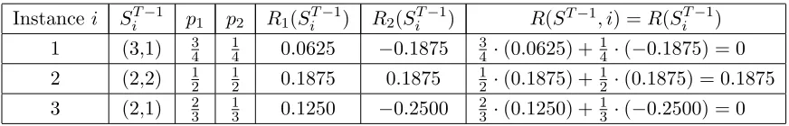
Instancei S_iT−1 p1 p2 R1(S_iT−1) R2(S_iT−1) R(ST−1, i) =R(S_iT−1) 1 (3,1) 3₄ 1₄ 0.0625 −0.1875 3₄·(0.0625) + 1₄·(−0.1875) = 0 2 (2,2) 1₂ 1₂ 0.1875 0.1875 ₂1·(0.1875) + 1₂·(0.1875) = 0.1875 3 (2,1) 2₃ 1₃ 0.1250 −0.2500 2₃·(0.1250) + 1₃·(−0.2500) = 0 Table 3: Calculation of the expected reward for the toy example in Table 1 according to

(12), (13) and (14).

absorbing state, namedSobs, to the original state space (15)and assume that, when the

bud-get allocation process finishes, the state must transit one more time to reachSobs regardless

of which action is taken. Hence, the original problem (8) becomes a MDP that generates a zero transition reward until the state entersSobs where the transition reward is

PK

i=1h(PiT).

Then, we define a potential-based shaping function (Ng et al., 1999) over this extended state space as Φ(St) = PK

i=1h(Pit) for St ∈ St and Φ(Sobs) = 0. After this, (4) can be viewed

as a new MDP whose transition reward equals that of (8) plus the shaping-reward function

Φ(S0)−Φ(S) when the state transits from S to S0. According to Theorem 1 in Ng et al. (1999),(4) and (8)have the same optimal policy. This provides an alternative justification for Proposition 4.

3.4 Optimal Policy via DP

With the MDP in place, we can apply the dynamic programming (DP) algorithm (a.k.a. backward induction) (Puterman, 2005) to compute the optimal policy:

1. Set VT−1(ST−1) = maxi∈{1,...,K}R(ST−1, i) for all possible states ST−1 ∈ ST−1. The optimal decision i∗_T₋₁(ST−1) is the decision i that achieves the maximum when the state isST−1.

2. Iterate for t = T −2, . . . ,0, compute the Vt(St) for all possible St ∈ St using the Bellman equation:

Vt(St)

= max

i

R(St, i) + Pr(yi= 1|St, i)Vt+1 St+ (ei,0)+ Pr(yi=−1|St, i)Vt+1 St+ (0,ei)

,

and i∗_t(St) is the ithat achieves the maximum.

The optimal policyπ∗= (i∗₀, . . . , i∗_T). For an illustration purpose, we use DP to calculate the optimal instance to be labeled next in the toy example in Section 2.1 under the uniform prior B(1,1) for all θi. Since we assume that there is only one labeling chance remaining, which corresponds to the last stage of DP, we should choose the instance i∗_T₋₁(ST−1) = arg max_i∈{1,...,K}R(ST−1, i). According to the calculation in Table 3, there is a unique optimal instance for labeling, which is the second instance.

(12)

4. Approximate Policies

Since DP is computationally intractable, approximate policies are needed for large-scale applications. The simplest policy is the uniform sampling (a.k.a, pure exploration), i.e., we choose the next instance uniformly and independently at random: it∼Uniform(1, . . . , K). However, this policy does not explore any structure of the problem.

With the decomposed reward function, our problem is essentially a finite-horizon Bayesian MAB problem. Gittins (1989) showed that Gittins index policy is optimal for infinite-horizon MAB with the discounted reward. It has been applied to the infinite-infinite-horizon ver-sion of problem (10) in Xie and Frazier (2013). Since our problem is finite-horizon, Gittins index is no longer optimal while it can still provide us a good heuristic index rule. However, the computational cost of Gittins index is very high: the state-of-art-method proposed by Nino-Mora (2011) requiresO(T6_{) time and space complexity.}

A computationally more attractive policy is the knowledge gradient (KG) (Gupta and Miescke, 1996; Frazier et al., 2008). It is essentially a single-step look-ahead policy, which greedily selects the next instance with the largest expected reward:

it= arg max i∈{1,...,K}

R(at_i, bt_i)=. a t i

at i+bti

R1(ati, bti) +

bt_i at

i+bti

R2(ati, bti)

. (16)

As we can see, this policy corresponds to the last stage in DP and hence KG policy is optimal if only one labeling chance is remaining.

When there is a tie, if we select the smallest indexi, the policy is referred todeterministic KG while if we randomly break the tie, the policy is referred torandomized KG. Although KG has been successfully applied to many MDP problems (Powell, 2007), it will fail in our problem as shown in the next proposition with the proof in the appendix.

Proposition 6 Assuming that a0_i andb0_i are positive integers and lettingE={i:a0_i =b0_i}, then the deterministic KG policy will acquire one label for each instance in E and then consistently obtain the label for the first instance even if the budget T goes to infinity.

According to Proposition 6, the deterministic KG is not a consistent policy, where the consistent policy refers to the policy that will provide correct labels for all instances (i.e.,

HT =H∗) almost surely whenT goes to infinity. We note that randomized KG policy can address this problem. However, from the proof of Proposition 6, randomized KG behaves similarly to the uniform sampling policy in many cases and its empirical performance is undesirable according to Section 8. In the next subsection, we will propose a new approx-imate allocation policy based on KG which is a consistent policy with superior empirical performance.

4.1 Optimistic Knowledge Gradient

The stage-wise reward can be viewed as a random variable with a two point distribution, i.e., with the probability p1 = _a₊a_b of being R1(a, b) and the probability p2 = _a₊b_b of being

(13)

Algorithm 1 Optimistic Knowledge Gradient

Input: Parameters of prior distributions for instances {a0_i, b0_i}K

i=1 and the budgetT. for t= 0, . . . , T−1do

Select the next instanceit to label according to:

it= arg max i∈{1,...,K}

R+(at_i, bt_i)= max(. R1(ati, bti), R2(ati, bti))

. (17)

Acquire the labelyit ∈ {−1,1}.

if yit = 1 then at_i+1

t =a

t it + 1, b

t+1 it =b

t it;a

t+1

i =ati, bti+1=bti for all i6=it. else

at_i+1 t =a

t it, b

t+1 it =b

t

it+ 1; a

t+1

i =ati, b t+1

i =bti for all i6=it. end if

end for

Output: The positive set HT ={i:aTi ≥bTi }.

a

b

1 2 3 4 5 6 7 8 9 10

10

9

8

7

6

5

4

3

2

1

0.05 0.1 0.15 0.2 0.25

Figure 2: Illustration ofR+(a, b).

In this section, we introduce a new index policy called “optimistic knowledge gradient” (Opt-KG) policy. The Opt-KG policy assumes that decision makers are optimistic in the sense that they select the next instance based on the optimistic outcome of the reward. As a simplest version of the Opt-KG policy, for any state (at_i, bt_i), the optimistic outcome of the rewardR+(at_i, bt_i) is defined as maximum over the reward of obtaining the label 1,R1(at_i, bt_i), and the reward of obtaining the label −1, R2(at_i, bt_i). Then the optimistic decision maker selects the next instanceiwith the largestR+(at_i, bt_i) as in (17) in Algorithm 1. The overall decision process using the Opt-KG policy is highlighted in Algorithm 1.

In the next theorem, we prove that Opt-KG policy is consistent.

(14)

Figure 3: Illustration of Conditional Value-at-Risk.

The key of proving the consistency is to show that when T goes to infinity, each instance will be labeled infinitely many times. We prove this by showing that for any pair of positive integers (a, b), R+(a, b) = max(R1(a, b), R2(a, b))>0 and R+(a, b) →0 when a+b→ ∞. As an illustration, the values of R+(a, b) are plotted in Figure 2. Then, by strong law of large number, we obtain the consistency of the Opt-KG as stated in Theorem 7. The details are presented in the appendix. We have to note that asymptotic consistency is the minimum guarantee for a good policy. However, it does not necessarily guarantee the good empirical performance for the finite budget level. We will use experimental results to show the superior performance of the proposed policy.

The proposed Opt-KG policy is a general framework for budget allocation in crowd labeling. We can extend the allocation policy based on the maximum over the two possible rewards (Algorithm 1) to a more general policy using the conditional value-at-risk (CVaR) (Rockafellar and Uryasev, 2002). We note that here, instead of adopting the CVaR as a risk measure, we apply it to the reward distribution. In particular, for a random variable

X with the support X (e.g., the random reward with the two point distribution), let α -quantile function be denoted asQα(X) = inf{x∈ X :α≤FX(x)}, whereFX(·) is the CDF of X. The value-at-risk VaRα(X) is the smallest value such that the probability that X is less than (or equal to) it is greater than (or equal to) 1−α: VaRα(X) =Q1−α(X). The conditional value-at-risk (CVaRα(X)) is defined as the expected reward exceeding (or equal to) VaRα(X). An illustration of CVaR is shown in Figure 3.

For our problem, according to Rockafellar and Uryasev (2002), CVaRα(X) can be ex-pressed as a simple linear program:

CVaRα(X) = max {q1≥0,q2≥0}

q1R1+q2R2, s.t. q1≤

1

αp1, q2 ≤

1

αp2, q1+q2 = 1.

(15)

own experience, α → 0 usually has a better performance in our problem especially when the budget is very limited. Therefore, for the sake of presentation simplicity, we introduce the Opt-KG using max(R1, R2) (i.e.,α →0 in CVaRα(X)) as the selection criterion.

Finally, we highlight that the Opt-KG policy is computationally very efficient. For K

instances withT units of the budget, the overall time and space complexity areO(KT) and

O(K) respectively. It is much more efficient that the Gittins index policy which requires

O(T6) time and space complexity. 4.2 Discussions

It is interesting to see the connection between the idea of making the decision based on the optimistic outcome of the reward and the UCB (upper confidence bounds) policy (Auer et al., 2002) for the classical multi-armed bandit problem as described in Section 3.3. In particular, the UCB policy selects the next arm with the maximumupper confidence index, which is defined as the current average reward plus the one-sided confidence interval. As we can see, the upper confidence index can be viewed as an “optimistic” estimate of the reward. However, we note that since we are in a Bayesian setting and our stage-wise rewards are artificially created and thus not i.i.d. for each arm, the UCB policy (Auer et al., 2002) cannot be directly applied to our problem.

In fact, our Opt-KG follows a more general principle of “optimism in the face uncer-tainty” (Szita and L˝orincz, 2008). Essentially, the non-consistency of KG is due to its nature of pure exploitation while a consistent policy should typically utilizes exploration. One of the common techniques to handle the exploration-exploitation dilemma is to take an action based on an optimistic estimation of the rewards (see Szita and L˝orincz, 2008; Even-Dar and Mansour, 2001), which is the role R+(a, b) plays in Opt-KG.

For our problem, it is also straightforward to design the “pessimistic knowledge gradient” policy which selects the next instance it based on the pessimistic outcome of the reward, i.e., it= arg maxi R−(ati, bti)

.

= min(R1(at_i, bt_i), R2(at_i, bt_i)).However, as shown in the next proposition with the proof in the appendix, the pessimistic KG policy is inconsistent under the uniform prior.

Proposition 8 When starting from the uniform prior (i.e., a0_i = b0_i = 1) for all θi, the

pessimistic KG policy will acquire one label for each instance and then consistently acquire the label for the first instance even if the budget T goes to infinity.

Finally, we discuss some other possible choices of prior distributions. For presentation simplicity, we only consider the Beta prior for eachθi with the fixed parameters a0i andb0i. In practice, more complicated priors can be easily incorporated into our framework. For example, instead of using only one Beta prior, one can adopt a mixture of Beta distributions as the prior and the posterior will also follow a mixture of Beta distributions, which allows an easy inference about the posterior. As we show in the experiments (see Section 8.1.2), the uniform prior does not work well when the data is highly skewed in terms of class distribution. To address this problem, one possible choice is to adopt the prior p(θ) =

(16)

to the mixture Beta prior, one can adopt the hierarchical Bayesian approach which puts hyper-priors on the parameters in the Beta priors. The inference can be performed using empirical Bayes approach (Gelman et al., 2013; Robert, 2007). In particular, one can periodically re-calculate the MAP estimate of the hyper-parameters based on the available data and update the model, but otherwise proceed with the given hyper-parameters. For common choices of hyper-priors of Beta, please refer to Section 5.3 in Gelman et al. (2013). These approaches can also be applied to model the workers’ reliability as we introduced in the next Section. For example, one can use a mixture of Beta distributions as the prior for the workers’ reliability, where Beta(c,1) corresponds to reliable workers, Beta(1,1) to random workers and Beta(1, c) to malicious or poorly informed workers.

5. Incorporate Reliability of Heterogeneous Workers

In push crowdsourcing marketplaces, it is important to model workers’ reliability so that the decision maker could assign more instances to reliable workers. Assuming that there are M workers in a push marketplace, we can capture the reliability of thej-th worker by introducing an extra parameter ρj ∈ [0,1] as in (Dawid and Skene, 1979; Raykar et al., 2010; Karger et al., 2013b), which is defined as the probability of getting the same label as the one from a random fully reliable worker. Recall that the soft-label θi is the i-th instance’s probability of being labeled as positive by a fully reliable worker and let zij be the label provided by the j-th worker for the i-th instance. We model the distribution of

zij for given θi and ρj using the one-coin model (Dawid and Skene, 1979; Karger et al., 2013b):

=ρjθi+ (1−ρj)(1−θi); (18)

=ρj(1−θi) + (1−ρj)θi, (19)

where yi denotes the label provided a random fully reliable worker for the i-th instance. We also note that it is straightforward to extend the current one-coin model to a more complex two-coin model (Dawid and Skene, 1979; Raykar et al., 2010) by introducing a pair of parameters (ρj1, ρj2) to model thej-th worker’s reliability. In particular,ρj1 andρj2 are the probabilities of getting the positive and negative labels when a fully reliable worker provides the same label.

Here we make the following implicit assumption:

Assumption 9 We assume that different workers make independent judgments and, for each single worker, the labels provided by him/her to different instances are also independent.

(17)

j-th worker is poorly informed or misunderstands the instruction such that he/she always assigns wrong labels.

We assume that instances’ soft-label {θi}Ki=1 and workers’ reliability {ρj}Mj=1 are drawn from known Beta prior distributions: θi ∼ Beta(a0i, b0i) and ρj ∼ Beta(c0j, d0j). At each stage, we need to make the decision on both the next instance i to be labeled and the next worker j to label the instance i (we omit t in i, j here for notational simplicity). In other words, the action space A = {(i, j) : (i, j) ∈ {1, . . . , K} × {1, . . . , M}}. Once the decision is made, the distribution of the outcome zij is given by (18) and (19). Given the prior distributions and likelihood functions in (18) and (19), the Bayesian Markov Decision process can be formally defined as in Section 3. Similar to the homogeneous worker setting, the optimal inferred positive setHT takes the form ofHT ={i:PiT ≥0.5}as in Proposition 2 with P_it = Pr(i ∈ H∗|F_t) = Pr (θi ≥0.5|Ft). The value function V(S0) still takes the form of (8), which can be further decomposed into the sum of stage-wise rewards in (9) using Proposition 4. Unfortunately, in the heterogeneous worker setting, the posterior distributions ofθi andρj are highly correlated with a sophisticated joint distribution, which makes the computation of stage-wise rewards in (9) much more challenging. In particular, given the priorθi ∼Beta(a0_i, b0_i) and ρj ∼Beta(c0_j, d0_j), the posterior distribution of θi and

ρj given the label zij =z∈ {−1,1} takes the following form:

p(θi, ρj|zij =z) =

Pr(zij =z|θi, ρj)Beta(a0i, b0i)Beta(c0j, d0j) Pr(zij =z)

, (20)

where Pr(zij =z|θi, ρj) is the likelihood function defined in (18) and (19) and

Pr(zij = 1) =E(Pr(zij = 1|θi, ρj)) =E(θi)E(ρj) + (1−E(θi))(1−E(ρj))

= a 0 i

a0_i +b0_i c0_j c0_j+d0_j +

b0_i a0_i +b0_i

d0_j c0_j+d0_j.

As we can see, the posterior distribution p(θi, ρj|zij = z) no longer takes the form of the product of the distributions of θi and ρj and the marginal posterior of θi is no longer a Beta distribution. As a result, P_it does not have a simple representation as in (5), which makes the computation of the reward function much more difficult as the number of stages increases. Therefore, to apply our Opt-KG policy to large-scale applications, we need to use some approximate posterior inference techniques.

(18)

Algorithm 2 Optimistic Knowledge Gradient for Heterogeneous Workers Input: Parameters of prior distributions for instances {a0_i, b0_i}K

i=1 and for workers

{c0_j, d0_j}M

j=1. The total budgetT. for t= 0, . . . , T−1do

1. Select the next instanceit to label and the next worker jt to label it according to:

(it, jt) = arg max (i,j)∈{1,...,K}×{1,...,M}

R+(ati, b t i, c

t j, d

t j)

.

= max(R1(ati, b t i, c

t j, d

t j), R2(a

t i, b

t i, c

t j, d

t j))

.

(21)

2. Acquire the labelzitjt ∈ {−1,1}of the i-th instance from thej-th worker.

3. Update the posterior by setting:

at_i+1 t = ˜a

t

it(zitjt) b

t+1 it = ˜b

t

it(zitjt) c

t+1 jt = ˜c

t

jt(zitjt) d

t+1 jt = ˜d

t

jt(zitjt),

and all parameters fori6=it and j6=jt remain the same. end for

Output: The positive set HT ={i:aTi ≥bTi }.

assuming the conditional independence of θi and ρj:

p(θi, ρj|zij =z)≈p(θi|zij =z)p(ρj|zij =z).

We further approximate p(θi|zij =z) and p(ρj|zij =z) by two Beta distributions:

p(θi|zij =z)≈Beta(˜ai(z),˜bi(z)), p(ρj|zij =z)≈Beta(˜cj(z),d˜j(z)),

where the parameters ˜ai(z), ˜bi(z), ˜cj(z), ˜dj(z) are computed using moment matching with the analytical form presented in the appendix. After this approximation, the new posterior distributions of θi and ρj still have the same structure as their prior distribution, i.e., the product of two Beta distributions, which allows a repeatable use of this approximation every time when a new label is collected. Moreover, due to the Beta distribution approximation of p(θi|zij = z), the reward function takes a similar form as in the previous setting. In particular, assuming at a certain stage, θi has the posterior distribution Beta(ai, bi) and

ρj has the posterior distribution Beta(cj, dj). The reward of getting positive and negative labels for thei-th instance from thej-th worker are presented in (22) and (23):

R1(ai, bi, cj, dj) =h(I(˜ai(z= 1),˜bi(z= 1)))−h(I(ai, bi)), (22)

R2(ai, bi, cj, dj) =h(I(˜ai(z=−1),˜bi(z=−1)))−h(I(ai, bi)). (23) With the reward in place, we present Opt-KG for budget allocation in the heterogeneous worker setting in Algorithm 2. We also note that due to the variational approximation of the posterior, establishing the consistency results of Opt-KG becomes very challenging in the heterogeneous worker setting.

6. Extensions

(19)

important extensions, where for both extensions, Opt-KG can be directly applied as an approximate policy. We note that for the sake of presentation simplicity, we only present these extensions in the noiseless homogeneous worker setting. Further extensions to the heterogeneous setting are rather straightforward using the technique from Section 5.

6.1 Utilizing Contextual Information

When the contextual information is available for instances, we could easily extend our model to incorporate such an important information. In particular, let the contextual information for the i-th instance be represented by a p-dimensional feature vector xi ∈ Rp. We could

utilize the feature information by assuming a logistic model for θi:

θi =.

exp{hw,xii} 1 + exp{hw,xii}

,

wherew is assumed to be drawn from a Gaussian priorN(µ₀,Σ0). At thet-th stage with the current state (µ_t,Σt), the decision maker determines the instanceitand acquire its label

yit ∈ {−1,1}. Then we update the posteriorµt+1 andΣt+1 using the Laplace method as in Bayesian logistic regression (Bishop, 2007). Variational methods can be applied to further accelerate the posterior update (Jaakkola and Jordan, 2000). The details are provided in the appendix.

6.2 Multi-Class Categorization

Our MDP formulation can also be extended to deal with multi-class categorization problems, where each instance is a multiple choice question with several possible options (i.e., classes). More formally, in a multi-class setting with C different classes, we assume that the i-th instance is associated with a probability vectorθi = (θi1, . . . θiC), whereθicis the probability that the i-th instance will be labeled as the class c by a random fully reliable worker and PC

i=1θic = 1. We assume that θi has a Dirichlet prior θi ∼ Dir(α0i) and the initial state

S0 is a K ×C matrix with α0_i as its i-th row. At each stage t with the current state

St, we determine the next instance it to be labeled and collect its label yit ∈ {1, . . . , C},

which follows the categorical distribution: p(yit) =

QC

c=1θ I(y_it=c)

itc . Since the Dirichlet is

the conjugate prior of the categorical distribution, the next state induced by the posterior distribution is: S_it+1

t =S

t

it +δyit andS

t+1

i =Sit for all i6=it. Hereδc is a row vector with one at thec-th entry and zeros at all other entries. The transition probability is:

Pr(yit =c|S

t_{, i}

t) =E(θitc|S

t_{) =} α t itc

PC

c=1αtitc .

We denote the true set of instances in class c by H_c∗ = {i : θic ≥ θic0,∀c0 6= c}. By a

similar argument as in Proposition 2, at the final stage T, the estimated set of instances belonging to classc is

H_cT ={i:P_icT ≥P_icT0,∀c06=c},

where P_ict = Pr(i ∈ H_c∗|Ft) = Pr(θic ≥ θic0, ∀ c0 6= c|St). We note that if the i-th

(20)

index c so that {H_cT}C

c=1 forms a partition of {1, . . . , K}. Let Pit = (Pit1, . . . , PiCt ) and

h(Pt_i) = max1≤c≤CPict. The expected reward takes the form of:

R(St, it) =E h(Pti+1t )−h(P

t it)|S

t_{, i} t

.

With the reward function in place, we can formulate the problem into a MDP and use DP to obtain the optimal policy and Opt-KG to compute an approximate policy. The only computational challenge is how to calculate P_ict efficiently so that the reward can be evaluated. We present an efficient method in the appendix. We can further use Dirichlet distribution to model workers reliability as in Liu and Wang (2012). Using multi-class Bayesian logistic regression, we can also incorporate contextual information into the multi-class setting in a straightforward manner.

7. Related Works

Categorical crowd labeling is one of the most popular tasks in crowdsourcing since it requires less effort of the workers to provide categorical labels than other tasks such as language translations. Most work in categorical crowd labeling are solving a static problem, i.e., inferring true labels and workers’ reliability based on a static labeled data set (Dawid and Skene, 1979; Raykar et al., 2010; Liu and Wang, 2012; Welinder et al., 2010; Whitehill et al., 2009; Zhou et al., 2012; Liu et al., 2012; Gao and Zhou, 2013). The first work that incorporates diversity of worker reliability is by Dawid and Skene (1979), which uses EM to perform the point estimation on both worker reliability and true class labels. Based on that, Raykar et al. (2010) extended (Dawid and Skene, 1979) by introducing Beta prior for workers’ reliability and features of instances in the binary setting; and Liu and Wang (2012) further introduced Dirichlet prior for modeling workers’ reliability in the multi-class setting. Our work utilizes the modeling techniques in these two static models as basic building blocks but extends to dynamic budget allocation settings.

(21)

metrics, such a balance could be very subjective. Furthermore, the MDP framework in Kamar et al. (2012) cannot distinguish different workers. To the best of our knowledge, there is no existing method that characterizes theoptimal allocation policy for finiteT. In this work, with the MDP formulation and DP algorithm, we characterize the optimal policy for budget allocation in crowd labeling under any budget level.

We also note that the budget allocation in crowd labeling is fundamentally different from noisy active learning (Settles, 2009; Nowak, 2009). Active learning usually does not model the variability of labeling difficulties among instances and assumes a single (noisy) oracle; while in crowd labeling, we need to model both instances’ labeling difficulty and different workers’ reliability. Secondly, active learning requires the feature information of instances for the decision, which could be unavailable in crowd labeling. Finally, the goal of the active learning is to label as few instances as possible to learn a good classifier. In contrast, for budget allocation in crowd labeling, the goal is to infer the true labels for as many instances as possible.

In fact, our MDP formulation is essentially a finite-horizon Bayesian multi-armed bandit (MAB) problem. While the infinite-horizon Bayesian MAB has been well-studied and the optimal policy can be computed via Gittins index (Gittins, 1989), for finite-horizon Bayesian MAB, the Gittins index rule is only an approximate policy with high computational cost. The proposed Opt-KG and a more general conditional value-at-risk based KG could be gen-eral policies for Bayesian MAB. Recently, a Bayesian UCB policy was proposed to address a different Bayesian MAB problem (Kaufmann et al., 2012). However, it is not clear how to directly apply the policy to our problem since we are not updating the posterior of the mean of rewards as in Kaufmann et al. (2012). We note that our problem is also related to optimal stopping problem. The main difference is that the optimal stopping problem is infinite-horizon while our problem is finite-horizon and the decision process must stop when the budget is exhausted.

8. Experiments

In this section, we conduct empirical study to show some interesting properties of the proposed Opt-KG policy and compare its performance to other methods. We observe that several commonly used priors such as the uniform prior (Beta(1,1)), Jeffery prior (Beta(1/2,1/2)) and Haldane prior (Beta(0,0)) for instances’ soft-label{θi}Ki=1lead to very similar performance. Therefore, we adopt the uniform prior (Beta(1,1)) unless otherwise specified. In addition, for the ease of comparison, the accuracy is defined as|HT∩H∗|+|(HT)c∩(H∗)c|

K ,

which is normalized between [0,1].

8.1 Simulation Study

(22)

0 0.2 0.4 0.6 0.8 1 2

4 6 8 10 12

Soft label (θ)

Labeling frequency

(a)T = 5K= 105

0 0.2 0.4 0.6 0.8 1 0

10 20 30 40 50 60

Soft label (θ)

Labeling frequency

(b) T = 15K= 315

0 0.2 0.4 0.6 0.8 1 0

50 100 150 200 250 300

Soft label (θ)

Labeling frequency

(c)T = 50K= 1050

Figure 4: Labeling counts for instances with different levels of ambiguity.

0 0.2 0.4 0.6 0.8 1 0.5

1 1.5 2 2.5 3 3.5

Worker reliability (ρ)

Labeling frequency

(a)T = 5K= 105

0 0.2 0.4 0.6 0.8 1 2

4 6 8 10

Labeling frequency

(b) T = 15K= 315

0 0.2 0.4 0.6 0.8 1 15

16 17 18 19 20 21

Labeling frequency

(c)T = 50K= 1050

Figure 5: Labeling counts for workers with different levels of reliability.

8.1.1 Study on Labeling Frequency

We first investigate that, in the homogeneous noiseless worker setting (i.e., workers are fully reliable), how the total budget is allocated among instances with different levels of ambiguity. In particular, we assume there are K = 21 instances with soft-labels θ = (θ1, θ2, θ3, . . . , θK) = (0,0.05,0.1, . . . ,1). We vary the total budget T = 5K,15K,50K and report the number of times that each instance is labeled on average over 20 independent runs. The results are presented in Figure 4. It can be seen from Figure 4 that, more ambiguous instances with θ close to 0.5 in general receive more labels than those simple instances with θ close to 0 or 1. A more interesting observation is that when the budget level is low (e.g., T = 5K in Figure 4(a)), the policy spends less budget on those very ambiguous instances (e.g., θ= 0.45 or 0.5 ), but more budget on exploring less ambiguous instances (e.g.,θ= 0.35, 0.4 or 0.6). When the budget goes higher (e.g.,T = 15K in Figure 4(b)), those very ambiguous instances receive more labels but the most ambiguous instance (θ= 0.5) not necessarily receives the most labels. In fact, the instances withθ= 0.45 and

(23)

0 0.2 0.4 0.6 0.8 1 0

1 2 3 4 5

x

(a) Beta(0.5,0.5)

0 0.2 0.4 0.6 0.8 1 0

0.5 1 1.5

x

(b) Beta(2,2)

0 0.2 0.4 0.6 0.8 1 0

0.5 1 1.5 2

x

(c) Beta(2,1)

0 0.2 0.4 0.6 0.8 1 0

1 2 3 4

x

(d) Beta(4,1)

Figure 6: Density plot for different Beta distributions for generating each θi. Here, (a) represents there are more easier instances; (b) more ambiguous instances; (c) & (d) imbalanced class distributions with more positive instances.

Next, we investigate that, in the heterogeneous worker setting, how many instances each worker is assigned. We simulate K = 21 instances’ soft-labels as before and further simu-late workers’ reliabilityρ= (ρ1, ρ2, . . . , ρM) = (0.1,0.15, . . . ,0.5,0.505,0.515, . . . ,0.995) for

M = 59 workers. Such a simulation ensures that there are more reliable workers, which is in line with actual situation. We vary the total budget T = 5K,15K,50K and report the number of instances that each worker is assigned on average over 20 independent runs in Figure 5. As one can see, when the budget level goes up, there is clear trend that more reliable workers receive more instances.

8.1.2 Prior for Instances

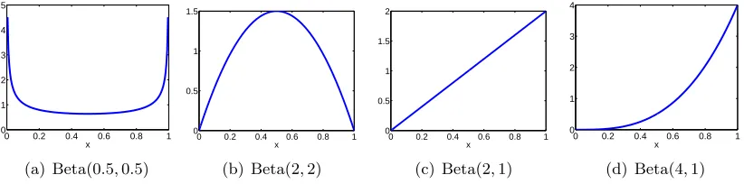
We investigate how robust Opt-KG is when using the uniform prior for each θi. We first simulateK = 50 instances with each θi ∼Beta(0.5,0.5), θi ∼Beta(2,2),θi ∼Beta(2,1) or

θi∼Beta(4,1). The density functions of these four different Beta distributions are plotted in Figure 6. For each generating distribution of θi, we compare Opt-KG using the uniform prior (Beta(1,1)) (in red line) to Opt-KG with the true generating distribution as the prior (in blue line). The comparison in accuracy with different levels of budget (T = 2K, . . . ,20K) is shown in Figure 7. As we can see, the performance of Opt-KG using two different priors are quite similar for most generating distributions except forθi ∼Beta(4,1) (i.e., the highly imbalanced class distribution). Whenθi∼Beta(4,1), the Opt-KG with uniform prior needs at leastT = 16Kunits of budget to match the performance of Opt-KG with true generating distribution as the prior. This result indicates that for balanced class distributions, the uniform prior is a good choice and robust to the underlying distribution of θi. For highly imbalanced class distributions, if a uniform prior is adopted, one needs more budget to recover from the inaccurate prior belief.

8.1.3 Prior on Workers

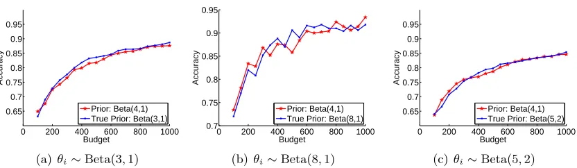
We investigate how sensitive the prior for the workers’ reliabilityρj is. In particular, we sim-ulateK = 50 instances with eachθi ∼Beta(1,1) andM = 100 workers withρj ∼Beta(3,1),

(24)

0 200 400 600 800 1000 0.86

0.88 0.9 0.92 0.94 0.96 0.98

Budget

Accuracy

Uniform Prior: Beta(1,1) True Prior: Beta(0.5,0.5)

(a)θi∼Beta(0.5,0.5)

0 200 400 600 800 1000 0.7

0.75 0.8 0.85 0.9 0.95

Budget

Accuracy

Uniform Prior: Beta(1,1) True Prior: Beta(2,2)

(b) θi∼Beta(2,2)

0 200 400 600 800 1000 0.75

0.8 0.85 0.9 0.95

Budget

Accuracy

(c)θi∼Beta(2,1)

0 200 400 600 800 1000 0.85

0.9 0.95 1

Budget

Accuracy

(d) θi∼Beta(4,1)

Figure 7: Comparison between Opt-KG using the uniform distribution and true generating distribution as the prior.

0 0.2 0.4 0.6 0.8 1 0

0.5 1 1.5 2 2.5 3

x

(a) Beta(3,1)

0 0.2 0.4 0.6 0.8 1 0

2 4 6 8

x

(b) Beta(8,1)

0 0.2 0.4 0.6 0.8 1 0

0.5 1 1.5 2 2.5

x

(c) Beta(5,2)

0 0.2 0.4 0.6 0.8 1 0

1 2 3 4

x

(d) Beta(4,1)

Figure 8: Density plot for different Beta distributions for generating ρj. The plot in (d) is the one that we use as the prior.

(25)

0 200 400 600 800 1000 0.65

0.7 0.75 0.8 0.85 0.9 0.95

Budget

Accuracy

Prior: Beta(4,1) True Prior: Beta(3,1)

(a)θi∼Beta(3,1)

0 200 400 600 800 1000 0.7

0.75 0.8 0.85 0.9 0.95

Budget

Accuracy

(b) θi∼Beta(8,1)

0 200 400 600 800 1000 0.65

0.7 0.75 0.8 0.85 0.9 0.95

Budget

Accuracy

(c)θi∼Beta(5,2)

Figure 9: Comparison between Opt-KG using Beta(4,1) and true generating distribution prior as the prior.

generating distribution of θi, we compare the Opt-KG policy using the prior (Beta(4,1)) (in red line) to the Opt-KG with the true generating distribution as the prior (in blue line). The comparison in accuracy with different levels of budget (T = 2K, . . . ,20K) is shown in Figure 9. From Figure 9, we observe that the performance of Opt-KG using two different priors are quite similar in all different settings. Hence, we will use Beta(4,1) as the prior when the true prior of workers is unavailable.

8.1.4 Performance Comparison Under the Homogeneous Noiseless Worker Setting

We compare the performance of Opt-KG under the homogeneous noiseless worker setting to several other competitors, including

1. Uniform: Uniform sampling.

2. KG(Random): Randomized knowledge gradient (Frazier et al., 2008).

3. Gittins-Inf: A Gittins-indexed based policy proposed by Xie and Frazier (2013) for solving an infinite-horizon Bayesian MAB problem where the reward is discounted by

δ. Although it solves a different problem, we apply it as a heuristic by choosing the discount factor δ such that T = 1/(1−δ).

4. NLU: The “new labeling uncertainty” method proposed by Ipeirotis et al. (2013).

We note that we do not compare to the finite-horizon Gittins index rule (Nino-Mora, 2011) since its computation is very expensive. On some small-scale problems, we observe that the finite-horizon Gittins index rule (Nino-Mora, 2011) has the similar performance asGittins-Inf in Xie and Frazier (2013).

(26)

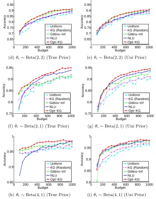
true generating distribution as the prior. From Figure 10, the proposed Opt-KG outperforms all the other competitors in most settings regardless the choice of the prior. For θi ∼ Beta(0.5,0.5), NLU matches the performance of Opt-KG; and forθi ∼Beta(2,2), Gittins-inf matches the performance of Opt-KG. We also observe that the performance of randomized KG only slightly improves that of uniform sampling.

8.1.5 Performance Comparison Under the Heterogeneous Worker Setting

We compare the proposed Opt-KG under the heterogeneous worker setting to several other competitors:

1. Uniform: Uniform sampling.

2. KG(Random): Randomized knowledge gradient (Frazier et al., 2008).

3. KOS:The randomized budget allocation algorithm in Karger et al. (2013b).

We note that several competitors for the homogeneous worker setting (e.g., Gittins-inf and NLU) cannot be directly applied to the heterogeneous worker setting since they fail to model each worker’s reliability.

We simulate K = 50 instances with each θi ∼ Beta(1,1) and M = 100 workers with

ρj ∼Beta(4,1), ρj ∼Beta(3,1),ρj ∼Beta(8,1) or ρj ∼Beta(5,2) (see Figure 8). For each of the four settings, we vary the total budget T = 2K,3K, . . . ,20K and report the mean of accuracy for 20 independently generated sets of parameters. For the last three settings, we report the comparison among different methods when either using Beta(4,1) prior or the true generating distribution forρj as the prior. From Figure 11, the proposed Opt-KG outperforms all the other competitors regardless the choice of the prior.

8.2 Real Data

(27)

0 200 400 600 800 1000 0.75 0.8 0.85 0.9 0.95 Budget Accuracy Uniform KG (Random) Gittins−Inf NLU Opt−KG

(a)θi∼Beta(1,1) (True Prior)

0 200 400 600 800 1000 0.8 0.85 0.9 0.95 1 Budget Accuracy Uniform KG (Random) Gittins−Inf NLU Opt−KG

(b) θi∼Beta(0.5,0.5) (True Prior)

0 200 400 600 800 1000 0.8 0.85 0.9 0.95 1 Budget Accuracy Uniform KG (Random) Gittins−Inf NLU Opt−KG

(c)θi∼Beta(0.5,0.5) (Uni Prior)

0 200 400 600 800 1000

0.65 0.7 0.75 0.8 0.85 0.9 0.95 Budget Accuracy Uniform KG (Random) Gittins−Inf NLU Opt−KG

(d) θi∼Beta(2,2) (True Prior)

0 200 400 600 800 1000

0.65 0.7 0.75 0.8 0.85 0.9 0.95 Budget Accuracy Uniform KG (Random) Gittins−Inf NLU Opt−KG

(e)θi∼Beta(2,2) (Uni Prior)

0 200 400 600 800 1000

0.75 0.8 0.85 0.9 0.95 Budget Accuracy Uniform KG (Random) Gittins−Inf NLU Opt−KG

(f)θi∼Beta(2,1) (True Prior)

0 200 400 600 800 1000

0.75 0.8 0.85 0.9 0.95 Budget Accuracy Uniform KG (Random) Gittins−Inf NLU Opt−KG

(g)θi∼Beta(2,1) (Uni Prior)

0 200 400 600 800 1000

0.85 0.9 0.95 1 Budget Accuracy Uniform KG (Random) Gittins−Inf NLU Opt−KG

(h) θi∼Beta(4,1) (True Prior)

0 200 400 600 800 1000

0.8 0.85 0.9 0.95 1 Budget Accuracy Uniform KG (Random) Gittins−Inf NLU Opt−KG

(i)θi∼Beta(4,1) (Uni Prior)

Figure 10: Performance comparison under the homogeneous noiseless worker setting.

(28)

0 200 400 600 800 1000 0.4 0.5 0.6 0.7 0.8 0.9 Budget Accuracy Uniform KG (Random) KOS Opt−KG

(a)ρj∼Beta(4,1) (True Prior)

(b) ρj∼Beta(3,1) (True Prior)

(c) ρj ∼ Beta(3,1) (Beta(4,1)

Prior)

0 200 400 600 800 1000

0.4 0.5 0.6 0.7 0.8 0.9 1 Budget Accuracy Uniform KG (Random) KOS Opt−KG

(d)ρj∼Beta(8,1) (True Prior)

0 200 400 600 800 1000

0.4 0.5 0.6 0.7 0.8 0.9 1 Budget Accuracy Uniform KG (Random) KOS Opt−KG

(e)ρj∼Beta(8,1) (Beta(4,1) Prior)

0 200 400 600 800 1000

0.4 0.5 0.6 0.7 0.8 0.9 Budget Accuracy Uniform KG (Random) KOS Opt−KG

(f)ρj∼Beta(5,2) (True Prior)

0 200 400 600 800 1000

0.4 0.5 0.6 0.7 0.8 0.9 Budget Accuracy Uniform KG (Random) KOS Opt−KG

(g)ρj∼Beta(5,2) (Beta(4,1) Prior)

Figure 11: Performance comparison under the heterogeneous worker setting.

Budget T 2K = 1,600 4K = 3,200 6K = 4,800 10K = 8,000

Opt-KG 1.09 2.19 3.29 5.48

Gittins-inf 25.87 35.70 45.59 130.68

Table 4: Comparison in CPU time (seconds)

(29)

0 2000 4000 6000 8000 0.65

0.7 0.75 0.8 0.85 0.9 0.95

Budget

Accuracy Uniform

KG (Random) Gittins−Inf NLU Opt−KG

(a) RTE: Homogeneous Noiseless Worker

0 2000 4000 6000 8000 0.65

0.7 0.75 0.8 0.85 0.9 0.95

Budget

Accuracy

Uniform KG (Random) KOS

Opt−KG

(b) RTE: Heterogeneous Worker

Figure 12: Performance comparison on the real data set.

and in fact, slightly downgrades a little bit. This is mainly due to the restrictiveness of the experimental setting. In particular, since the experiment is conducted on a fixed data set with partially observed labels, the Opt-KG cannot freely choose instance-worker pairs especially when the budget goes up (i.e., the action set is greatly restricted). According to our experience, such a phenomenon will not happen on experiments when labels can be obtained from any instance-worker pair. Comparing Figure 12(b) to 12(a), we also observe that Opt-KG under the heterogeneous worker setting performs much better than Opt-KG under the homogeneous worker setting, which indicates that it is beneficial to incorporate workers’ reliability.

9. Conclusions and Future Work

In this paper, we propose to address the problem of budget allocation in crowd labeling. We model the problem using the Bayesian Markov decision process and characterize the optimal policy using the dynamic programming. We further propose a computationally more attractive approximate policy: optimistic knowledge gradient. Our MDP formulation is a general framework, which can be applied to binary or multi-class, contextual or non-contextual crowd labeling problems in either pull or push crowdsourcing marketplaces.

(30)

can be provided. Further, since the proposed Opt-KG is a fairly general approximate policy for MDP, it is also interesting to apply it to other statistical decision problems.

Acknowledgments

We would like to thank Qiang Liu for sharing the code for KOS method; Jing Xie and Peter Frazier for sharing their code for computing infinite-horizon Gittins index; John Platt, Chris Burges and Kevin Murphy for helpful discussions; and anonymous reviewers and the associate editor for their constructive comments on improving the quality of the paper.

Appendix A. Proof of Results

In this section, we provide the proofs of the main results of our paper.

A.1 Proof of Proposition 2

The final positive setHT is chosen to maximize the expected accuracy conditioned on FT:

HT = arg max

H E

K

X

i=1

(1(i∈H)1(i∈H∗) +1(i6∈H)1(i6∈H∗))

F_T !

. (24)