How to extract weak values from a mesoscopic electronic system

(will be inserted by the editor)

How to extract weak values from a mesoscopic

electronic system

Iliya Esin

·

Alessandro Romito

·

Yuval

Gefen

Received: date / Accepted: date

Abstract

Weak value (WV) protocols may lead to extreme expectation values

that are larger than the corresponding orthodox expectation values. Recent works

have proposed to implement this concept in nano-scale electronic systems. Here

we address the issue of how one calibrates the setup in question, maximizes the

measurement’s sensitivity, and extracts distinctly large WVs. Our concrete setup

consists of two Mach-Zehnder interferometers (MZIs): the “system” and the

“de-tector”. Such setups have already been implemented in experiment.

Keywords

weak value

·

weak measurement

·

Mach-Zehnder interferometer

1 Introduction and motivation

Strong measurement in quantum mechanics leads to the collapse of the measured

system’s wave function [16]. The challenge of performing a non-invasive

measure-ment is interesting both from the view point of foundations of quantum mechanics,

and for concrete applications (e.g. quantum computation). Weakly measuring an

observable, while weakly disturbing the system, provides only partial information

on the state of the latter. Weak measurements, due to their backaction, can be

ex-ploited for quantum feedback schemes [28, 24, 26] and conditional measurements.

The latter entail WV protocols [1] and derivatives thereof.

A standard two-step WV protocol consists of a weak measurement step (of the

observable

A

), followed by a strong one (of

B

), [

A, B

]

6

= 0. The outcome of the

first is conditional on the result of the second (postselection),

i.e., one admits the

I.Esin

Department of Condensed Matter Physics, The Weizmann Institute of Science, Rehovot 76100, Israel

A. Romito

Department of Physics, Lancaster University, Lancaster, LA1 4YB, United Kingdom

Y. Gefen

Department of Condensed Matter Physics, The Weizmann Institute of Science, Rehovot 76100, Israel

Φ

_sys

QPC A

QPC B

S2

S1

D2

D1

λ

𝑽

𝑺𝟏

𝑰

𝑫𝟏

arm 1 arm 2

Detector

𝛀

𝐿2

𝐿1

Fig. 1 (Color online) A weakly detected MZI. The average reading of the detector,Ω, is linearly proportional (to leading order in system–detector coupling,λ) to the total electric charge on arm 2 of the interferometer at the time of the measurement. (If the detector is a

current–carrying quantum point contact (QPC), thenΩ(t) is equal toΩ(t)∼Rt+τf l/2

t−τf l/2 I(t

0_)dt0_,

where I(t) is the current through the QPC and τf l = L2/v, with L2 being the length of

arm 2 andvthe velocity of the chiral edge mode). The strong follow-up measurement detects the charge (current pulse) arriving at the drain D1. Registering the outcome of the first measurement is subsequently conditioned on detecting a ‘click’ inD1. This is the WV of the charge in arm 2.

outcome of the weak measurement of

A

provided the result of the (strong)

measure-ment of

B

coincides with a prescribed value,

h

A

i

_{W V}

=

Tr{A·ΠB}

Tr{ΠB}

, with

Π

B

being

the projection operator on the postselected subspace. WVs have been observed in

experiments [18, 17, 11, 9]. Their unusual expectation values [1] may be utilized for

various purposes, including weak signal amplification [5, 22, 3, 23, 7, 29], quantum

state discrimination [14, 30], and non-collapsing observation of virtual states [19].

There have been recent proposals to implement WV protocols in the context of

solid state systems [21, 20, 6]. Apart from the realization with superconducting

qubits in resonant cavity[9], setups made up of two (electrostatic interaction

cou-pled) MZIs, operating in the quantum Hall regime, are of particular importance,

given their immediate experimental availability [12, 25] and their versatile and

controllable nature. In such setups one MZI plays the role of “the system”, the

other being “the detector”.

Shpitalnik

et al.[21] have implemented, in principle, a WV protocol in this

setup, and have shown that the outcome of such measurement may produce a

complete tomography of the WV measured in the system’s MZI. An exhaustive

analysis of the correlated signal in this system has been reported in the single

particle regime[6], and the many body effects on the weak to strong measurement

crossover have been classified [8]. The fact that such a protocol is amenable to

ex-perimental verification [25] has been undermined by the lack of a concrete manual

on how to implement it.

[image:2.595.72.416.74.201.2]

2 The system: a MZI

Our system consists of a MZI depicted schematically in Fig. 1. Electrons are

in-jected from the source contact

S

1, kept at a finite voltage bias

V

S1, and are

col-lected at drain

D

1. The other terminals of the interferometers are grounded. The

Quantum Point Contacts (QPCs) A and B allow tunnelling of the electrons

be-tween arms 1 and 2 of the system; the electrons collected at

D

1 are the result of

the interference of different electron trajectories, and are sensitive to the magnetic

flux

Φ

sys. A detector is electrostatically coupled to the charge in arm 2 of the

interferometer. At this stage we refer to a general detector, weakly coupled to the

system.

We consider explicitly the case where the bias current fed into the MZI is

di-luted (for example, one modifies the setup depicted in Fig. 1 such that most

elec-trons emitted from the source

S

1 are backscattered before arriving in the MZI). In

that case, the width of an electron’s wave packet is much smaller than the distance

between two consecutive electrons. Moreover, we require that the time

separa-tion between successive injecsepara-tions of non-equilibrium electrons (

τ

VS1,

2

π

~

/eV

S1

is

much larger than the electron’s time-of-flight through the interferometer’s arm[27]:

τ

VS1

τ

f l

. To reduce adverse decoherence effects one may consider the limit of low

temperature, low voltage bias, and nearly symmetric interferometers (i.e., nearly

equal arm lengths). The conditions are met in actual experiments [12, 25].

The first step of our protocol consists of weakly measuring the electric charge

Q

2, flowing through arm 2 of the interferometer. This (weak) measurement is

performed as a snapshot at time

t

W

of the electric charge along arm 2. The

follow-up (strong) measurement detects the charge arriving at the drain

D

1 with a delay,

t

delay

, due to the finite propagation time of the charge from the weak detector to

D

1. The measurement itself consists of integrating the current pulse over a window

of time, [

t

W

+

t

delay

, t

W

+

t

delay

+

τ

f l

], which corresponds to the time of flight of

an electron through arm 2 (the latter is of length

L

2;

τ

f l

=

L

2

/v

, where

v

is the

Fermi velocity of the non-equilibrium electrons). We denote this integrated current

by

τ

f l

I

D1. Under the conditions of diluted injected current specified above, the

postselection signal,

I

D1, can reveal the detection of one or no electrons collected

at

D

1, we then condition the acceptance of the first measurement of

Q

2

on a ‘click’

in

D

1. Therefore the weak value of the charge on arm 2 is

h

Q

2

i

_{W V}

=

Q

2(

t

W

)

·

I

D1(

t

W

+

t

delay

+

12

τ

f l

)

h

I

D1

i

.

(1)

We now relate the abstract WV defined above to a measurable quantity. We

as-sume that (to leading order in system–detector coupling) the average signal of the

detector is linearly proportional to measured charge,

i.e.,

h

δΩ

i

=

S h

Q

2

i

, where

Ω

is the signal of the detector with

δΩ

,

Ω

−

Ω

_h

Q2i=0

and

S

is the sensitivity of the

detector defined as

S

_,

∂

h

Ω

i

∂

h

Q

2

i

.

(2)

We define the measured

h

Q

2

i

M_{W V}

as

h

Q

2

i

M_{W V}

,

1

S

h

δΩ

·

I

D1

i

h

I

D1

i

S4

S3

D4

D3

Φ

det

QPC C

QPC D

Φ

sys

QPC A

QPC B

S2

S1

D2

D1

λ

𝑽

𝑺𝟒

𝑽

𝑺𝟏

𝑰

𝑫𝟒

𝑰

𝑫𝟏

MZI

_det

MZI

_sys arm 1 arm 2 arm 3 arm 4 𝐿4

𝐿3

𝐿2

𝐿1

(a)

𝑉𝑆1

𝐼𝐷4

𝑉𝑆4

𝐼𝐷1

𝑉𝑄𝑃𝐶 𝐵

𝑉𝑄𝑃𝐶 𝐴

𝑉𝑀𝐺𝑠𝑦𝑠

𝑉𝑀𝐺𝑑𝑒𝑡

𝑉𝑄𝑃𝐶 𝐷

𝑉𝑄𝑃𝐶 𝐶

(b)

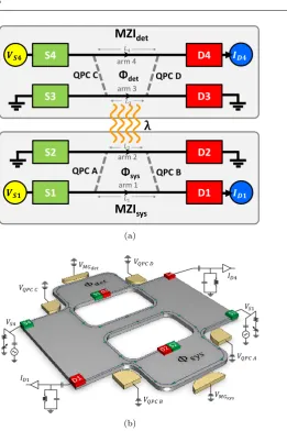
Fig. 2 (Color online) A concrete realization of the setup. (a) A schematic layout. (b) A realistic design. The system and the detector are realized by MZIsysand MZIdet, which are weakly (with

strengthλ) electrostatically coupled through arms 2 and 3. The sourcesS1 andS4 are biased with the voltagesVS1andVS4respectively, while the signals are measured inD1 andD4. The

contactsS2,D2,S3 andD3 are connected to the ground. The gate voltagesVQPC A-Dcontrol

the inter-arm tunneling amplitudes of electrons near the respective QPC. The modulation gate biasesVM Gsys (VM Gdet) control the effective magnetic fluxesΦsys (Φdet) by modifying the

areas encircled by electronic trajectories along the device.

We expect the latter to be proportional to the WV

h

Q

2

i

_{W V}

(c.f Eq. (1)).

3 The detector: a MZI

[image:4.595.75.337.71.464.2]

S4

S3

D4

D3

Φ

_det

Φ

_sys

S2

S1

D2

D1

λ

|

𝜓

₁𝑠𝑦𝑠

|

𝜓

₂𝑠𝑦𝑠

|

𝜓

₃𝑠𝑦𝑠

|

𝜓

₄𝑠𝑦𝑠

|

𝜓

1𝑑𝑒𝑡

|

𝜓

2𝑑𝑒𝑡

|

𝜓

3𝑑𝑒𝑡

|

𝜓

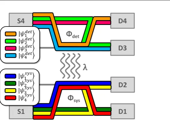
4𝑑𝑒𝑡

Fig. 3 (Color online) Electronic trajectories along MZIs. The underlying scattering elec-tronic wavefunction can be constructed as an entangled product of elecelec-tronic trajectories in MZIsysand in MZIdet. Those are depicted schematically by different colors. cf. Appendix A for

explicit expressions for the electronic trajectories.

MZI is tuned, analogously with the system MZI, to have a diluted incident current

and a time-separation between incident electrons larger than the time-of-flight

across the interferometer. The current of the detector integrated over

τ

f l

,

τ

f l

I

D4,

is sensitive to a charge on arm 2, and serves as a

pointer variable

— It plays the role

of

Ω

in the general formulation of the previos section. The (weak) signature of the

system–detector interaction is a small additional phase gain of the wavefunction

when a pair of electrons flow simultaneously along the arms 2 and 3 respectively[6,

15].

Therefore, the definition of

h

Q

2

i

MW V

(Eq. (3)) in the case of MZI as a detector

(cf. Fig. 2) reads

h

Q

2

i

M_{W V}

=

1

S

_h

I

D4

I

D1

i

h

I

D1

i

− h

I

D4

i

00

.

(4)

It requires the measurement of the current–current correlator

h

I

D4

I

D1

i

, the

aver-age current in

D

1,

h

I

D1

i

, and the average current in

D

4 when the transmission

of QPC A is set to zero,

h

I

D4

i

00

. The value of

[image:5.595.77.359.80.296.2]

4 The system-detector coupling

To gain physical insight on the detector’s response and determine its proper

cali-bration we resort to a two-particle picture (one electron passing through MZIsysand

another in MZIdet). The model is a valid description of the interaction between

the system and detector electrons in the regime of diluted electron currents we are

considering.

The two-particle scattering state,

|

Ψ

sys,det

i

, near the drains (after the QPCs

B and D) can be expressed in terms of partial electronic trajectories (cf. Fig. 3)

as,

|

Ψ

sys,det

i

=

X

ij

e

iλij

_c

sys

i

|

ψ

sys

i

i

c

det j

ψ

det j

E

,

(5)

where

c

sys_i

(

c

deti

) are amplitudes of the trajectories through MZIsys(MZIdet)

omit-ting the coupling between the interferometers (cf. Appendix A), and

λ

ij

=

λ,

(

i

= 1

∨

4)

∧

(

j

= 1

∨

4)

0

,

o.w.

is the weak coupling term (

λ

1). The WV of

Q

2

(cf. Eq. (1)) may be expressed

in terms of the amplitudes

c

i

as

h

Q

2

i

_{W V}

=

h

Q

2

i

₀

c

sys₄

c

sys₄

+

c

sys₂

.

(6)

where

h

Q

2

i

₀

≈

e

2_V

S1L2

2π~v

is the average excess charge on the segment

L

2. Similarly,

we define

h

Q

3

i

_{W V}

=

h

Q

3

i

₀

c

det1

c

det

1

+

c

det3

,

(7)

with

h

Q

3

i

₀

≈

e

2

VS4L3

2π~v

, as the weak value of the charge on arm 3 conditioned on a

signal in

D

4. With these definitions the signal in

D

4 to first order in

λ

is given by

(cf. Appendix B)

h

I

D4

i

=

h

I

D4

i

0

1 + 2˜

λ

Im

n

h

Q

3

i

_{W V}

h

h

Q

2

i

+

D

Q

bg₂

Eio

,

(8)

where ˜

λ

=

λ/

h

Q

2

i

₀

h

Q

3

i

₀

and

h

Q

2

i

=

h

Q

2

i

₀

|

c

sys₁

|

2

+

|

c

sys₄

|

2

is the

out-of-equilibrium and

D

Q

bg₂

E

is the background charge on arm 2,

h

I

D4

i

₀

=

h

Q

3

i

₀

/τ

f l

c

det₁

+

c

det₃

2

is the current measured at

D

4 in the absence of interaction (

λ

= 0). We obtain

also the explicit expression for Eq. (4) (cf. Apeendix B), given by

h

Q

2

i

M_{W V}

=

2˜

λ

h

I

D4

i

0

S

Im

h

Q

2

i

_{W V}

h

Q

3

i

_{W V}

− h

Q

3

i

.

(9)

From the analysis it also follows that the sensitivity of the MZI detector (cf.

Eq. (2)) is

S

= 2˜

λ

h

I

D4

i

₀

Im

h

Q

3

i

_{W V}

,

(10)

with the explicit expression

S

= 2

h

Q

3

i

2₀

λ/τ

˜

f l

c

det₁

c

det₃

sin ˜

φ

. Here ˜

φ

is the total

phase difference between the trajectories

ψ

₁det

and

ψ

₃det

0.0 0.5 1.0 1.5 2.0 0.0

0.5 1.0

𝐼

𝐷4 00

𝐼

𝐷4

11

Δ 𝐼

𝐷4

Φ

𝑑𝑒𝑡

/Φ

0

Current through the detector

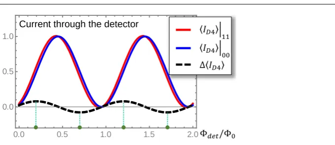
Fig. 4 (Color online) Calibration of the detector. The QPCs C and D are set to half trans-mission (|tC| = |tD| = 1/

√

2), ˜λ = 0.05π. The currents are measured in units of hQ3i0.

The red (blue) curve corresponds to the signal in D4 when both QPC A and QPC B are fully transmitting (reflecting),hID4i

11(hID4i

00). The black dashed curve is their difference:

∆hID4i,hID4i

11 −hID4i

00. The detector is maximally sensitive at the extremas of∆ hID4i.

Those points are highlighted by green dots.

The first requirement may be achieved by individually adjusting the gate voltages

of the QPCs. To set the phase ˜

φ

of the detector to the maximal sensitivity point

we employ a calibration protocol discussed below.

5 Calibration of the detector and extraction of weak values

Let us assume the QPCs are already tuned to the half transmission point. Here

we present a calibration protocol for the phase ˜

φ

governing the interference signal

registered in the detector. In the first step of this protocol, one sets QPC A of

the system(!) (by tuning the gate voltage

V

QPC A) to ‘full reflection’ (no current

through both QPC A and QPC B

1

, cf. Fig. 2), and measures the current

h

I

D4

i

00

as function of the detector’s flux

Φ

det

/Φ

0, where

Φ

0

=

h/e

is the magnetic flux

quantum. Evidently the signal is independent of the system’s flux

Φ

sys

, and of

the transmission of QPC B. In this configuration the amplitudes for trajectories

|

ψ

sys₁

i

and

|

ψ

₄sys

i

vanish and consequently

h

Q

2

i

= 0. In the second step both

QPC A and QPC B are tuned to the opposite limit of ‘full transmission’ (a charge

arriving from

S

1 is deflected, with probability 1, to arm 2 (cf. Fig. 2)), setting

the weight of the trajectories

|

ψ

₂sys

i

and

|

ψ

₃sys

i

to zero. In this configuration the

current in MZIsysflows through arm 2 and the charge

h

Q

2

i

reaches its maximal

value,

h

Q

2

i

_max

. In this limit, the current measured in the detector is denoted

h

I

D4

i

11

.

A representative plot of

h

I

D4

i

for the two tunings:

h

I

D4

i

00

and

h

I

D4

i

11

respectively, and their difference

∆

h

I

D4

i

,

h

I

D4

i

11

− h

I

D4

i

[image:7.595.76.416.76.223.2]

as a function of magnetic flux

Φ

det

. The maximal sensitivity of the detector is

achieved when one sets the magnetic flux to extremal points of

∆

h

I

D4

i

. Values of

the latter are depicted in the figure.

The calibration process prescribes the values of the sensitivity

S

(cf. Eq. (10)),

h

Q

3

i

_{W V}

(cf. Eq. (7),

h

I

D4

i

₀

and

h

Q

3

i

=

h

Q

3

i

₀

c

det₁

2

+

c

det₄

2

(cf. equations

following Eq.(8)). It turns out that the calibration at maximal sensitivity yields

Re

h

Q

3

i

_{W V}

=

h

Q

3

i

. Using the latter equality and Eq. (10) we rewrite Eq. (9)

as

h

Q

2

i

M_{W V}

=

Re

h

Q

2

i

_{W V}

(at maximal sensitivity)

,

(11)

which sets the relation between the measured (real) quantity and the abstract

definition of (complex) weak values. Consulting Eq. (4) we conclude that we can

conveniently get rid of the factor 1

/

S

by defining the normalized WV,

h

Q

2

i

M

W V

,

h

Q

2

i

MW V

h

Q

2

i

M_{W V}

11

.

(12)

Here

h

Q

2

i

MW V

11

is the measured

h

Q

2

i

W V

, when both QPCs A and B are set to full

transmission. For this tuning, it follows that

h

Q

2

i

M_{W V}

11

=

h

Q

2

i

_{W V}

=

h

Q

2

i

_max

.

Eq. (12) involves only measurable quantities and serves to operatively identify

weak values beyond the range allowed by unconditioned measurements.

6 Results and discussion

The present analysis is aimed at implementing the general framework of WV

protocol [1] to a representative electronic system. The latter is experimentally

ac-cessible [25], rendering the present protocol amenable to experimental verification.

We have focused on one central aspect of WV, namely the possibility to obtain

expectation values (a.k.a.

weak values) that lie beyond the range of possible

out-comes of strong measurement [16] (the latter implies the collapse of the system’s

wave function). Specifically, our setup consists of a “system” and a “detector”

(MZIsysand MZIdet, cf. Fig. 2) which are electrostatically weakly coupled. The

detector is tuned to measure the charge transmitted through one of the system

interferometer’s arms (a weak “which path” measurement [2, 13, 10, 4]).

Intuition based on strong measurement procedure would suggest that when

one electron is injected into the system’s MZI, the normalized charge that can

be measured on one of the interferometer arms is anything between 0 and 1.

By contrast, WV protocol allows us to obtain values which are above this value

(“charge larger than 1” or even

negative). The results shown in Fig. 5 make it

clear that as far as weak values are concerned, both conventional values (that

conform to “allowed values” of strong measurement)

and

exceptional values which

lie beyond the interval [0

,

1] are possible.

Specifically consider Figures 5a and 5b. We show that

h

Q

2

i

M

W V

may grow

beyond the range of values allowed by a strong measurement of

Q

2, which involves

the collapse of the system’s wavefunction. This is highlighted by a different (gray)

color of the 3D plot. Figures 5c and 5d show

h

Q

2

i

M

|𝑡𝐵|

(b)

(c) _(d)

Φ𝑠𝑦𝑠/Φ0 |𝑡𝐵|

𝑄2 𝑊𝑉𝑀

(a)

𝑄2 𝑊𝑉𝑀

𝑄2 𝑊𝑉𝑀 _{𝑡𝐵 = 0.79} 𝑄2 𝑊𝑉𝑀

𝑡𝐵 = 0.62

Φsys= 0.94Φ0

Φsys= 0. 4Φ0

Fig. 5 (Color online) The normalized WV,hQ2i

M

W V, as a function of transmission amplitude

of QPC B,|tB|, and the flux,Φsys/Φ0. The transmission of QPC A is set to|tA|= √1₂, and

˜

λ= 0.05π. An overall phaseδ= 0.1π, representing the asymmetry of the interferometer’s arms is included, implying that the interference pattern is not symmetric aroundΦ0/2. (a). A 3D

plot ofhQ2i

M

W V as a function oftB andΦsys/Φ0. (b).hQ2i

M

W V as a function of the real and

the imaginary parts oftBexp (Φsys/Φ0). The yellow colored region corresponds to values that

fall within the conventional range, [0,1], while the gray regions underline the observability of “exceptional values” that lie beyond this range. The dashed lines correspond to specific cuts along|tB|= 0.62 (red),|tB|= 0.79 (blue),Φsys= 0.94Φ0(orange), andΦsys= 0.4Φ0(black).

Those are depicted in (c) vs.Φsys/Φ0and in (d) vs.|tB|, with the same respective colors.

plot, for

|

t

B

|

= 0

.

62 and

|

t

B

|

= 0

.

79 as a function of

Φ

sys

/Φ

0, and

Φ

sys

= 0

.

94

·

Φ

0

and

Φ

sys

= 0

.

4

·

Φ

0

as a function of

|

t

B

|

. We note that the WV may become

exceedingly large (positive or negative) for a proper choice of the parameters.

In the procedure outlined above, we have put special emphasis on how the

measured values of current and current correlations should be calibrated to fit

with the weak value formalism. It would be interesting to repeat this analysis

having in mind variations of our setup (e.g., replacing the MZI detector by a QPC

or a current carrying quantum dot).

[image:9.595.74.415.75.309.2]

A Appendix 1: Explicit expressions for electronic trajectories

A.1 Solution to the single particle Hamiltonian

Here we solve the single-particle problem for a single MZI (suppose MZIsysfrom figure 2) and

expand the solution in partial electronic trajectories (cf. Fig. 3). We begin with the single particle Schr¨odinger equation

i~ ∂ ∂t− ˆ H

Ψ= 0 (13)

whereΨ=

ψ1(x, t)

ψ2(x, t)

, and ˆ HΨ=  

iv∂xψ1(x, t) +Pα=A,B

h_Γ∗

α 2 δ(x−x

+

1α)ψ2(x−1α, t) + Γ_α∗

2 δ(x−x

−

1α)ψ2(x+1α, t)

i

iv∂xψ2(x, t) +P_α=A,B

h

Γα 2 δ(x−x

+ 2α)ψ1(x

−

2α, t) + Γα

2 δ(x−x

−

2α)ψ1(x

+ 2α, t)

i 

.

(14) Hereψ1(x, t) andψ2(x, t) denote the wavefunctions in the corresponding arms 1 and 2, Γα

represents the tunneling term associated with theα-th QPC, connecting pointsx1αandx2α,

α=A, B(cf. Fig. 6));x±_{= lim}

ε→0x±ε.Γα may be related to the scattering amplitudes

through Eqs. (16).

This problem is diagonal in the scattering basis

Ψk,l(x, t) =

1

√

Le

ik(x−vt)







νl , x∈I

˘

SAνl , x∈II

˘

SBνl, x∈III

. (15)

Here the Latin numerals denote the various sectors of the MZI: I - left to QPC A, II - between

QPC A and B, III- right of QPC B, ˘Sα=

rα−t∗α

tα rα

is the scattering matrix at QPCαand

the scattering amplitudes are

rα=

(2v2_{)− |Γ}

α|2

(2v2_{) +|Γ}

α|2

(16a)

tα= 4ivΓα

(2v2_{) +|Γα|}2, (16b)

for the symmetric MZI case (x1B−x1A = x2B−x2A). The index l = 1,2 denotes two

orthogonal solutionsν1=

1 0

andν2=

0 1

that correspond to the scattering state incident

fromS1 orS2.

A.2 Explicit expressions for the coefficients

c

i

The probability of the particle incident fromS1 to be detected inD1 can be presented using the path integral formalism as

PS1→D1=

Z C

DΨ eiS{Ψ}/~

2 , (17)

where C represents all the trajectories from S1 to D1, and ci,eiS{Ψi}/~ _{is the weight of}

the corresponding trajectory. The same argument may be repeated for probabilitiesPS1→D2,

PS2→D1, andPS2→D2to include all the trajectories depicted in Fig. 3. The explicit

Φ

S2

S1

D2

D1

arm 1 arm 2

𝑥1𝐴

𝑥2𝐴 𝑥2𝐵

𝑥1𝐵

I II III

L

Fig. 6 (Color online) A schematics of a MZI. The pointsx1α and x2α,α=A, B at QPCs

A and B are connected by the tunneling terms Γα. The Latin numerals denote the various

sectors of the MZI: I - left to QPC A, II - between QPC A and B, III- right of QPC B.

summarize the results. Up to unimportant orbital phases

csys₁ =−t∗ArB (18a)

csys₂ =rArB (18b)

csys₃ =−rAt∗B (18c)

csys₄ =−t∗AtB (18d)

cdet1 =−tCt∗D (18e)

cdet2 =rCtD (18f)

cdet3 =rCrD (18g)

cdet4 =tCrD. (18h)

B Appendix 2: Derivation of expectation values and correlators

Here we derive explicit expressions for expectation values of operators that appear throughout the manuscript. For simplicity we assume a symmetric MZI (L1 =L2,L3 =L4) operating

in the low frequency, zero temperature regime, where the quantum state does not vary much over the time of the experiment, hence is almost steady. Thus, in this regime, all quantities are essentially time independent. We evaluate the expectation values by computing a trace of the operator with respect to the initial density matrix,ρi = |S1, S4i hS1, S4|describing

two particles, which are taken fom out-of equilibrium distribution,and which are incident from the biased sourcesS1 andS4 (cf. Fig. 2). At the end of this appendix (cf. Section B.4) we add a contribution from the equilibrium, background sea of electrons below the Fermi level. Throughout this section, the charge operators associated with each MZI are normalized to have no physical units. The latter may be recovered at the end, multiplying the normalized charge byhQii0 (i= 2,3) (those are defined following Eqs. (6) and (7)).

B.1 Derivation of equations (6) and (7)

Writing explicitly the expectation values appearing in eq. (1), we come up with the expression

hQ2iW V =

hS1, S4|Q2ID1|S1, S4i hS1, S4|ID1|S1, S4i

, (19)

whereID1 =|D1i hD1|. To leading order in the coupling,λ(cf. eq. (5)), the two MZIs may

be considered as decoupled, and the trace over MZIdetstates (|S4i hS4|) is trivial. Hence the

expression reads

hQ2iW V =

hS1|Q2|D1i

[image:11.595.74.422.76.184.2]

The operatorQ2is proportional to a projection operator that selects only partial wavepackets

ψ1_sys

andψ4_sys

(cf. Fig. 3). Onlyψ1_sys

has support atD1 and contributes to the numerator. The denominator includes two contributions,

ψ_sys2

and ψ_sys4

. It follows that

hQ2iW V =

csys₄

csys₄ +csys₂ . (21)

The derivation of an expression forhQ3iW V,

hQ3·ID4i

hID4i (eq. (7)) is similar.

B.2 Expression for the system–detector current correlator

Here we derive the expression forhID1ID4ito leading order in the couplingλ. The expression

for the non-equilibrium currents correlator reads

hID1ID4i=hS1, S4|ID1ID4|S1, S4i. (22)

We plug in the explicit expressions for the currents,ID1=|D1i hD1|andID4=|D4i hD4|to

obtain,

hID1ID4i=|hS1, S4|D1, D4i|2. (23)

We note that due to charge conservation and the assumption of a steady state, the sum of the currents on the two arms (between the QPCs) of any MZI, is equal to the total current that flows into the MZI. For example, for MZIsys,

IS1=I1+I2, (24)

where IS1 denotes an operator that measures current flow through S1, and I1(2) measure

currents at arbitrary points on arm 1 (2) (cf. Fig 2). Next, we integrate Eq. (24) over the time-of flight time-of electron in the MZI. Integration time-ofIS1over this time yields the total charge that

flows into the MZI during the time-of-flight. The latter is noiseless according to our assumptions and therefore is proportional to the identity (exactly one electron has been injected fromS1). The integration ofI1(2)yields the fraction of charge that when to arm 1(2),Q1(2). It follows

from the above that

Q1+Q2=1, (25)

where we have usedτf lIS1=1in dimensionless units. A similar identity may be obtained for

MZIdet,

Q3+Q4=1. (26)

Next, we insert those unit operators into Eq. (23), which yields the expression

hID1ID4i=

hS1, S4|Q1Q3+Q1Q4+

+Q2Q3+Q2Q4|D1, D4i

2 . (27)

Each element in the sum is diagonal in the basis of trajectories, and can be evaluated employing the wavefunction (5). It follows that

hID1ID4i=

hQ1iS1;D1hQ3iS4;D4+hQ1iS1;D1hQ4iS4;D4+

+eiλhQ2iS1;D1hQ3iS4;D4+hQ2iS1;D1hQ4iS4;D4

2 , (28)

where we have introduced the notationhQi_S;D=hS|Q|Di. Using the identities (25) and (26), and expanding to leading order inλ, we arrive at the expression

hID1ID4i=

h1iS1;D1h1iS4;D4+iλhQ2iS1;D1hQ3iS4;D4

2

. (29)

Simplifying it, employing the relationshID1i0≡

h1iS1;D1

2

,hID4i0≡

h1iS4;D4

2

(see for ex-ample Eq. (23) and eq. (20)), we obtain

hID1ID4i=hID1i0hID4i0 1 + 2λIm

B.3 Expressions for the current expectation values

Here we compute the expressions for the current expectation values. To do so, we employ the charge conservation in a steady state regime. We repeat the discussion following Eq. (25) that led to the identities

ID1+ID2=1 (31a)

ID3+ID4=1. (31b)

The latter may be employed to write

hID1i=hID1ID3i+hID1ID4i (32a) hID4i=hID2ID4i+hID1ID4i. (32b)

SincehID1ID4iwas found in eq. (30), one may follow the derivation in appendix B.2 to obtain

an expression forhID1ID3iandhID2ID4i. Plugging those results into Eq. (32) one ends up

with the equalities

hID1i=hID1i0 1 + 2λIm

hQ2iW V hQ3i (33a)

hID4i=hID4i0 1 + 2λIm

hQ3iW V hQ2i . (33b)

B.4 The contribution of the background charge

Above we have derived expressions for the average currents and current-current correlator in the presence of single particle taken from out-of-equilibrium distribution. In real life, there is background charge. The latter may interact with the incoming electrons, producing a shift in the measured signal. We consider the background charge as a noiseless constant that shifts the charge operator on each arm (Q2→Q2+

D

Qbg₂ E,Q3→Q3+

D

Qbg₃ E). We may now rewrite now eqs. (30) and (33) with the contribution of the background charge,

hID1i=hID1i0

1 + 2λImnhQ2iW V

h

hQ3i+

D

Qbg₃ Eio (34a)

hID4i=hID4i0

1 + 2λIm

n

hQ3iW V

h

hQ2i+

D Qbg₂

Eio

(34b)

hID4ID1i=hID4i0hID1i0

h

1 + 2λImnhhQ2iW V +

D

Qbg₂ Ei hhQ3iW V +

D

Qbg₃ Eioi (35)

(cf. Eq. (8)).

References

1. Y. Aharonov, D.Z. Albert, L. Vaidman, How the result of a measurement of a component of the spin of a spin- 1/2 particle can turn out to be 100. Phys. Rev. Lett.60(14) (1988). doi:10.1103/PhysRevLett.60.1351

2. I.L. Aleiner, N.S. Wingreen, Y. Meir, Dephasing and the Orthogonality Catastrophe in Tunneling through a Quantum Dot: The Which Path? Interferometer. Phys. Rev. Lett. 79(19) (1997). doi:10.1103/PhysRevLett.79.3740

3. N. Brunner, C. Simon, Measuring Small Longitudinal Phase Shifts: Weak Mea-surements or Standard Interferometry? Phys. Rev. Lett. 105(1), 010405 (2010). doi:10.1103/PhysRevLett.105.010405

5. P.B. Dixon, D.J. Starling, A.N. Jordan, J.C. Howell, Ultrasensitive Beam Deflection Mea-surement via Interferometric Weak Value Amplification. Phys. Rev. Lett.102(17), 173601 (2009). doi:10.1103/PhysRevLett.102.173601

6. J. Dressel, Y. Choi, A.N. Jordan, Measuring which-path information with cou-pled electronic Mach-Zehnder interferometers. Phys. Rev. B 85(4), 045320 (2012). doi:10.1103/PhysRevB.85.045320

7. J. Dressel, M. Malik, F.M. Miatto, A.N. Jordan, R.W. Boyd, Colloquium : Understanding quantum weak values: Basics and applications. Rev. Mod. Phys.86(1), 307–316 (2014). doi:10.1103/RevModPhys.86.307

8. I. Esin, A. Romito, Y.M. Blanter, Y. Gefen, Crossover between strong and weak measurement in interacting many-body systems. New. J. Phys. 18(1), 013016 (2016). doi:10.1088/1367-2630/18/1/013016

9. J.P. Groen, D. Rist`e, L. Tornberg, J. Cramer, P.C. de Groot, T. Picot, G. Johansson, L. Di-Carlo, Partial-Measurement Backaction and Nonclassical Weak Values in a Superconduct-ing Circuit. Phys. Rev. Lett.111(9), 090506 (2013). doi:10.1103/PhysRevLett.111.090506 10. S.A. Gurvitz, Measurements with a noninvasive detector and dephasing mechanism. Phys.

Rev. B56(23), 15215–15223 (1997). doi:10.1103/PhysRevB.56.15215

11. O. Hosten, P. Kwiat, Observation of the spin hall effect of light via weak measurements. Science319, 787–90 (2008). doi:10.1126/science.1152697

12. Y. Ji, Y. Chung, D. Sprinzak, M. Heiblum, D. Mahalu, H. Shtrikman, An electronic MachZehnder interferometer. Nature422, 415–418 (2003). doi:10.1038/nature01503 13. Y. Levinson, Dephasing in a quantum dot due to coupling with a quantum point contact.

Eur. Phys. Lett.39(3), 299–304 (1997). doi:10.1209/epl/i1997-00351-x

14. J.S. Lundeen, B. Sutherland, A. Patel, C. Stewart, C. Bamber, Direct measurement of the quantum wavefunction. Nature474, 188–91 (2011). doi:10.1038/nature10120

15. I. Neder, M. Heiblum, D. Mahalu, V. Umansky, Entanglement, Dephasing, and Phase Recovery via Cross-Correlation Measurements of Electrons. Phys. Rev. Lett.98(3), 036803 (2007). doi:10.1103/PhysRevLett.98.036803

16. J.V. Neumann, Mathematical Foundations of Quantum Mechanics (Investigations in physics (Princeton University Press), Princeton). 0691028931

17. G.J. Pryde, J.L. OBrien, A.G. White, T.C. Ralph, H.M. Wiseman, Measurement of Quantum Weak Values of Photon Polarization. Phys. Rev. Lett.94(22), 220405 (2005). doi:10.1103/PhysRevLett.94.220405

18. N.W.M. Ritchie, J.G. Story, R.G. Hulet, Realization of a measurement of a “weak value”. Phys. Rev. Lett.66(9), 1107–1110 (1991). doi:10.1103/PhysRevLett.66.1107

19. A. Romito, Y. Gefen, Weak measurement of cotunneling time. Phys. Rev. B90(8), 085417 (2014). doi:10.1103/PhysRevB.90.085417

20. A. Romito, Y. Gefen, Y.M. Blanter, Weak Values of Electron Spin in a Double Quantum Dot. Phys. Rev. Lett.100(5), 056801 (2008). doi:10.1103/PhysRevLett.100.056801 21. V. Shpitalnik, Y. Gefen, A. Romito, Tomography of Many-Body Weak

Val-ues: Mach-Zehnder Interferometry. Phys. Rev. Lett. 101(22), 226802 (2008). doi:10.1103/PhysRevLett.101.226802

22. D.J. Starling, P.B. Dixon, A.N. Jordan, J.C. Howell, Optimizing the signal-to-noise ratio of a beam-deflection measurement with interferometric weak values. Phys. Rev. A80(4), 041803 (2009). doi:10.1103/PhysRevA.80.041803

23. D.J. Starling, P.B. Dixon, N.S. Williams, A.N. Jordan, J.C. Howell, Continuous phase amplification with a Sagnac interferometer. Phys. Rev. A 82(1), 011802 (2010). doi:10.1103/PhysRevA.82.011802

24. R. Vijay, C. Macklin, D.H. Slichter, S.J. Weber, K.W. Murch, R. Naik, A.N. Korotkov, I. Siddiqi, Stabilizing Rabi oscillations in a superconducting qubit using quantum feedback. Nature490, 77–80 (2012). doi:10.1038/nature11505

25. E. Weisz, H.K. Choi, I. Sivan, M. Heiblum, Y. Gefen, D. Mahalu, V. Umansky, An elec-tronic quantum eraser. Science344(6190), 1363–6 (2014). doi:10.1126/science.1248459 26. H.M. Wiseman, G.J. Milburn,Quantum Measurement and Control(Cambridge University

Press, Cambridge, 2010). ISBN 0521804426

27. S.-C. Youn, H.-W. Lee, H.-S. Sim, Nonequilibrium Dephasing in an Elec-tronic Mach-Zehnder Interferometer. Phys. Rev. Lett. 100(19), 196807 (2008). doi:10.1103/PhysRevLett.100.196807

doi:10.1103/PhysRevB.72.245322

29. O. Zilberberg, A. Romito, Y. Gefen, Charge Sensing Amplification via Weak Values Mea-surement. Phys. Rev. Lett.106(8), 080405 (2011). doi:10.1103/PhysRevLett.106.080405 30. O. Zilberberg, A. Romito, D.J. Starling, G.A. Howland, C.J. Broadbent, J.C. Howell, Y.