Detecting bias due to input modelling in computer simulation

W. K. V. Chan, A. D’Ambrogio, G. Zacharewicz, N. Mustafee, G. Wainer, and E. Page, eds.

DETECTING BIAS DUE TO INPUT MODELLING IN COMPUTER SIMULATION

Lucy E. Morgan, Andrew C. Titman, David J. Worthington

Statistics and Operational Research Centre for Doctoral Training in Partnership with Industry Lancaster University

Lancaster, LA1 4YR, UK

Barry L. Nelson

Department of Industrial Engineering & Management Sciences Northwestern University

Evanston, IL 60208 USA

ABSTRACT

Bias due to input modelling is almost always assumed negligible and ignored. It is known that increasing the amount of real-world data available for modelling input processes causes this form of bias to decrease faster than the variance due to input uncertainty. However, this does not mean bias is irrelevant when considering the error in a simulation performance measure caused by input modelling. In this paper we present a response surface approach to bias estimation in simulation models along with a diagnostic test for identifying, with controlled power, bias due to input modelling of a size that would be concerning to a practitioner.

1 INTRODUCTION

Simulation models are driven by input distributions or processes. These input models are often built using real-world observations of the system of interest and are therefore always approximate due to the finite amount of available observations. This causes error in the output performance measures due to the non-linear form of simulation models. The mean squared error (MSE) about the simulation output due to input modelling can be broken down into variance, or “input uncertainty” (IU), and bias due to input modelling.

Methods for quantifying input uncertainty in simulation models exist. Song and Nelson (2015) and Cheng and Holland (1997) present methods for quantifying IU in simulation models with time homogeneous input distributions; this was extended by Morgan et al. (2016) to piecewise-constant non-stationary Poisson arrival processes. However, bias due to input modelling has, to date, been ignored, due to the fact that bias reduces faster than input uncertainty as the quantity of observations increase. To get a full picture of the total error in the simulation output due to input modelling it is not enough to consider IU alone. Bias can be small and therefore hard to accurately estimate without large simulation effort. But this does not mean bias is irrelevant. In context it may have a considerable impact on the error of the simulation response. For this reason we present a new diagnostic test that not only gives an estimate of bias, but has controlled power, 1−α2, of rejecting the null hypothesis if bias is more than a relevant threshold, γ. This may be

Our approach is focused on the design of the following two-sided hypothesis test

H0: Bias=0 vs. H1: Bias6=0

with type I error rate, or size, α1. The test will be set up to ensure controlled power, 1−α2, of rejecting

the null hypothesis when the absolute value of the true bias is greater than or equal toγ>0. This method

ensures that if, on conclusion of the test, the bias is found not to be relevant then the simulation practitioner can be confident that they do not need to consider bias further. Conversely, if a relevant bias is detected then further steps should be taken to include it in the analysis of total model risk.

We begin this paper with a discussion of the current literature in §2. In §3 the formulation of the diagnostic test is presented and an algorithm is given in §3.4. In §4.1 and §4.2 we evaluate the diagnostic test by considering simulation models with quadratic and non-quadratic response surfaces, respectively, and in §4.3 a realistic application of the method in a call centre setting is given. We conclude in §5.

2 BACKGROUND

As described in §1 we not only present a method for bias estimation, but also a diagnostic test with controlled power of identifying whether a relevant bias is present in the simulation output. This idea is common in the field of medical statistics for finding a relevant treatment effect with controlled power (Liu 1997). Although designing an experiment to satisfy certain power constraints is not a new idea, using it to create a simulation diagnostic for assessing whether bias is relevant has never before been tried.

Within our diagnostic test we make use of the delta method, giving an estimate of bias based upon a second-order Taylor Series approximation of the response function. Withers (1987) discussed this method and applied it for the purpose of bias reduction. We apply the delta method to quantify the bias in the output of a simulation model caused by input modelling; compared to other situations where a bias estimate may be required this has the additional complication of simulation noise. Alternative methods for bias quantification are the jackknife and the bootstrap. In the general case, without simulation noise, these methods were found inferior to the delta method in terms of computational efficiency in all but a few special cases where it could be said the jackknife method was comparable (Withers and Nadarajah 2014). In the context of simulation there may be a strict simulation budget, so computational efficiency can be very important.

To be able to use the delta approximation of bias we require evaluation of the Hessian matrix of second-order partial derivatives of the mean simulation response; this is simple if a closed form response function exists. But simulation models are usually unknown functions of their input parameters. Therefore to estimate these partial derivatives we propose using a central composite experimental design (CCD) to fit a response surface model as described by Montgomery (2013). This enables us to investigate the behaviour of the simulation response close to the true input parameter values.

We now present the diagnostic test for assessing whether bias due to input modelling is a relevant error about the simulation output.

3 DETECTING BIAS OF A RELEVANT SIZE

Bias due to input modelling is often small, requiring a large amount of simulation effort to accurately estimate. Although small, in context this bias may make a considerable contribution to the error about the simulation output. A practitioner may have in mind a value that they believe to be a worrying level of bias,

γ; this value is informed by the output of the nominal experiment. In this section we present a hypothesis

test that will detect, with controlled power, whether the absolute value of bias is greater than or equal toγ.

The method still requires an estimate of bias, but it is easier to test for bias than to estimate it accurately. We therefore require less simulation effort.

estimator; these values come together within the diagnostic test forming the test statistic. To estimate bias we start by considering the delta method approximation. This requires evaluation of the second-order partial derivatives of the response function (Nelson 2013). In reality, the simulation response is likely to be an unknown function of the input parameters with unknown partial derivatives. We therefore estimate the simulation response function by building a response surface model. Under the assumption that our response surface is locally quadratic, we use a CCD experimental design to fit this model, allowing estimation of the partial derivatives and therefore an estimate of the delta method approximation to bias, henceforth denoted

b b.

Given this bias estimator,bb, the key to our approach is in controlling the power of the hypothesis test so

we have a high probability of rejecting the null hypothesis when|bb| ≥γ is satisfied. This power is directly

controlled by the variance of the bias estimator which can be reduced in two ways: by increasing the number of replications at each design point or by increasing the width of the experimental design. Note that there are limitations to how far we can spread our experimental design before our quadratic approximation fails, whereas, in theory, we could increase our simulation effort at each design point endlessly. We therefore allow for a large number of replications at each design point and use the width of the experimental design to ensure the power holds. We next present the components of our bias detection approach.

3.1 The Delta Method

Let there beLparametric input distributions to the simulation with true input parametersθθθc={θ₁c,θ₂c, . . . ,θ_kc}; note that k≥L as some distributions may have multiple parameters. For some set of parameters θθθ, the

output of the jth replication of the simulation can be represented by

Yj(θθθ) =η(θθθ) +εj,

whereη(θθθ)is the expected value of the simulation response and we assumeεj∼(0,σ2(θθθ)), forj=1,2, . . . ,r,

representing the stochastic estimation error from replication to replication of the simulation.

For each of theLinput distributions,l=1,2, . . . ,L, we haveml real-world observations from which we

can find the maximum likelihood estimators (MLEs),θθθmle={θ₁mle,θ₂mle. . . ,θ_kmle}, of the input parameters.

Given these estimators, bias due to input modelling,b, is defined as

b=E[η(θθθmle)]−η(θθθc). (1)

Since θθθc is unknown, we approximate bias using the delta method approach as follows. Assuming the expected simulation response,η(·), is twice continuously differentiable aboutθθθc, it can be expanded as a Taylor Series to second-order

η(θθθmle)≈η(θθθc) +d(θθθmle)T∇η(θθθc) + 1

2!d(θθθ

mle₎T _H(θ θ

θc)d(θθθmle),

where d(θθθmle) = (θθθmle−θθθc) is the difference between the MLEs and true parameters, ∇η(θθθc) is the

(k×1) gradient vector of the response function and H(θθθc)represents the (k×k) Hessian matrix of second

derivatives with respect to the k input parameters. Using this Taylor series expansion an estimate of bias is given by

b=E[η(θθθmle)]−η(θθθc) ≈1

2E[d(θθθ

mle₎T_H(θ θ

θc)d(θθθmle)],

asd(θθθmle) = (θθθmle−θθθc)→0 in probability, due to the consistency of the MLEs. This gives, after some

matrix manipulation,

bapprox=1

2 tr(ΩH(θθθ

c_)),

the delta method approximation of bias, where tr()denotes the trace of a matrix andΩ=Var(θθθmle). When

the simulation response is an unknown function and the true input parametersθθθcare unknown, we estimate bapprox to give our estimate of bias

bb=

1

2tr(ΩbHb(θθθ

mle

)). (3)

For this we require estimates of both the covariance matrix of the input parameters and the Hessian matrix of second-order partial derivatives. The estimated covariance matrix,Ωb =Varc(θθθmle), will be obtained from

the real-world data and is from here forward assumed known. Estimating the Hessian is a little more tricky. We chose a response surface modelling approach, quantifying the curvature of the response surface by investigating the behaviour of the function close toθθθmle.

3.2 Fitting a Response Surface Model

Central to our method is the further assumption that, locally toθθθc, our response surface is quadratic and can be approximated by

η(θθθ)≈β0+θθθTβββ+

1 2θθθ

T

BBBθθθ,

whereβββ is the vector of coefficients belonging to the linear terms and BBB is the (k×k) matrix of coefficients

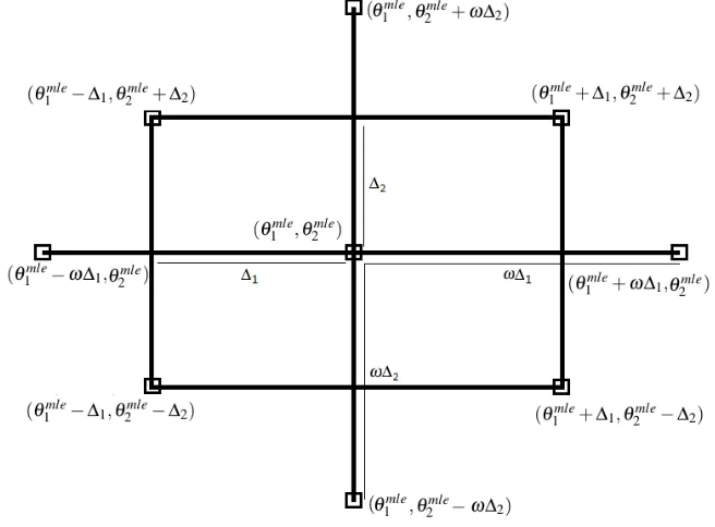
belonging to the interaction and quadratic terms. We will use a CCD centred atθθθmle to fit the response surface; see Figure 1 for an example of a 2-dimensional,k=2, design. We chose to use a CCD because they are well known and allow the estimation of higher-order regression coefficients which could be used to check the fit of the response surface. Within the experimental design, letnF denote the number of factorial

Figure 1: A CCD design with dimensionk=2.

points,nA the number of axial points andnCthe number replications of the centre point. The total number

of design points n is therefore n=nF+nA+nC=2k+2k+nC, which depends on the number of input

parameters,k. As suggested by Montgomery (2013) we let there be multiple design points at the centre,

point,i=1,2, . . . ,n, we completer replications of the simulation model. The total number of replications is thereforen×r.

As seen in Figure 1, we position the factorial and axial points relative to the centre point,θθθmle. Let∆i

be the distance to a factorial point from the centre point in the ith direction, i=1,2, . . . ,k, and similarly let τi be the distance to the axial points. We set

∆i=a q

Var(θmle

i ) and τi=ω∆i=aω q

Var(θmle i ),

whereais the number of standard deviations the factorial points are from the centre point in theithdirection. Hereωis the scaled distance from the centre to the axial points; we setω=p(√nFn−nF)/2 as suggested

by Dean and Voss (1999) for creating orthogonal designs, although we note here that due to the assumed quadratic nature of the response surface, orthogonality does not hold.

Given the averaged output of the simulation, ¯Y(θθθˆi), at each design pointi=1,2, . . . ,n, we use regression

analysis to evaluate the estimatesBBB, which in turn allows us to estimate the Hessian, whereb

ˆ

H(θθθmle) =     

2Bb₁₁ Bb₁₂ . . . Bb₁k b

B21 2Bb₂₂

..

. . ..

b

Bk1 2Bbkk

     ,

and therefore the bias, usingbb, as in Equation (3). The variance of this bias estimator, conditional on the

value ofΩb, can be expanded as follows

Var(bb) =Var

1

2tr(ΩbHb(θθθ

mle )) =1 4Var " 2 k

∑

BiiΩb_ii+ k

∑

k

∑

b

Bi jΩb_{i j} #

= k

∑

k

∑

Var(bBi j)Ωb2_{i j}+2 k

∑

k

∑

Cov(bBi j,Bblm)Ωbi jΩblm,

requiring the calculation of Var(BBBb), the variance-covariance matrix of regression coefficients belonging to

the interaction and quadratic terms. Given that we can estimate the stochastic estimation error,σb 2_{, from}

the nominal experiment, this matrix has special form

Var(bBii) = b σ2s ra4_Ωb2

ii

, Var(bBi j) = b σ2f ra4_Ωb

iiΩbj j

and Cov(Bbii,Bbj j) = b σ2g ra4_Ωb

iiΩbj j

,

which we will exploit later when it comes to setting the width of the CCD in our hypothesis test. Here,s,

f andg are constants independent ofa and Ωb. Note that Cov(bBi j,Bblm) =0 when i6= j andl6=mif we

use a CCD, therefore Var(bb) has the form

Var(bb) = σb 2

ra4 "

sk+f k

∑

k

∑

b Ω2_{i j}

b ΩiiΩbj j

+gk(k−1) #

. (4)

This variance estimator only accounts for the variability of the Hessian as Ωb, the covariance matrix, and b

At this point we have presented a method for estimating the bias about the simulation response caused by input modelling and have also provided a variance estimate associated with it. We could stop here but as was argued at the start of this section, testing for bias is easier than finding an accurate point estimate of it and requires less simulation effort. We will now present our key idea, a diagnostic test for detecting bias of relevant sizeγ with controlled power.

3.3 How to Detect a Relevant Bias

We begin by considering the following hypothesis test

H0:b=0 vs. H1:b6=0

with test statistic

T=q bˆ

Var(b)ˆ

.

This hypothesis test asks the question: is bias significantly different from 0? We shall assume that

ˆ

b−b q

Var(b)ˆ

∼N(0,1) =Z. (5)

We want an experimental design where the following significance and power hold

P[T<Zα1/2,T>Z1−α1/2

b=0] =α1 (6)

P[T<Zα1/2,T>Z1−α1/2

|b| ≥γ]≥1−α₂ (7)

given a relevant bias,γ, set by the practitioner. We know that Equation (6) is guaranteed by (5). Constraint (7) says that if bias is relevant we want controlled power, probability 1−α₂of rejecting the null hypothesis. This holds when

q

Var(b)ˆ ≤ γ Z₁−α2−Zα1/2

. (8)

We can therefore control the power of our experiment using the variance about our bias estimator, Var(b)ˆ . Recall from Equation (4) that Var(b)ˆ is a function of the width of the CCD, set usinga, andr, the number of replications at each design point, along withΩb andσ_b2, constants estimated in the nominal experiment.

As previously mentioned, due to the limitations on how far we can spread our design until our quadratic assumption breaks down, we choose to fixr at some appropriately large number and find the value of a

where our power holds.

Returning to Equation (4) we see that a, the parameter controlling the width of the design, can be factored out of Var(b)ˆ . Thus our problem simplifies to findingasuch that Constraint (7) holds which gives

a≥ "

b σ2t2

rγ2 sk+f k

∑

k

∑

b Ω2_{i j}

b ΩiiΩb_{j j}

+gk(k−1) !#1₄

. (9)

Given a that satisfies Constraint (9) we can set up a CCD for use within the hypothesis test which will detect with controlled power, 1−α2, a relevant bias, if the bias due to input modelling is truly at leastγ.

3.4 Algorithm

Preliminary Step. Estimateθθθc andΩbyθθθmle andΩb. Run the nominal experiment to estimateσ2 by σ_b2.

Setγ, a bias we wish to detect,α1 the size of the test and 1−α2 the power.

1. Set r, the number of replications at each design point. To find a such that the power holds we must first evaluate s,f and g. Initially let a=1, noting that any positive value would suffice; create the

n × 1+2k+k(k₂−1)

design matrix X, centred at(0,0, . . . ,0) for convenience with

∆i=a q

Var(θmle

i )andτi=ω∆i, for i=1,2, . . . ,k. GivenX, evaluates, f andg as follows s= (XTX)−1

[(k+1)(₂k+2),(k+1)(₂k+2)]∆

4

k, f = (XTX)_[−k1+2,k+2]∆

2 1∆22,

g= (XTX)−1

[(k+1)(₂k+2)−1,(k+1)(₂k+2)]∆

2 k−1∆2k

and thus evaluate the value of afor which the power holds using Equation (9). 2. Re-build the design matrixX givenafor which the power holds.

3. For iin 1 ton: Runr replications of the simulation at design point,θθθi, corresponding to rowiof

the design matrix; average over ther replications to find ¯Y(θθθi).

4. Using the simulation output from the n design points, ¯Y(θθθi) for i=1,2, . . . ,n, extract BBB fromb (XTX)−1XTYYY¯(θθθ), givingBb₁₁,Bb₁₂, . . . ,Bb_(k−1)k,Bb_kk.

5. EvaluateHb(θθθmle); thus evaluatebband Var(bb).

6. Calculate the test statistic, T=√ bb

Var(bb)

. If|T| ≥Z₁−α1/2 is satisfied reject the null hypothesis.

4 EMPIRICAL EVALUATION

In this section we will evaluate the diagnostic test presented in this paper by considering how well the power holds: firstly in a system where the simulation response surface is truly quadratic, and then for a tractable M/M/1/C queueing model. Finally we illustrate the use of the diagnostic test in a realistic call centre setting to show how in practice the diagnostic test could be used, and suggest follow-up actions for when a relevant bias is found.

4.1 A Truly Quadratic Model

Consider a quadratic response function. As an example, whenk=2 let the response function be given by

η(θθθ) =2+3θ1+θ2+4θ1θ2+θ₁2+2θ₂2. (10)

Here we letθ₁c andθ₂c be the true mean parameters from the following bivariate normal distribution

X1,X2∼N

(θ₁c,θ₂c)T,

ξ₁2 0

0 ξ₂2

with Cov(θ₁mle,θ₂mle) =0 and Var(θ_imle) =ξ_i2/m. Given this response function we know the Hessian

matrix exactly, therefore the delta approximation givesbapprox=ξ₁2/m+2ξ₂2/mwhich is exact since (10)

is quadratic.

Let us now assume that the response function, η(θθθ), is unknown to us. We wish to evaluate the performance of the diagnostic test when the underlying response surface is truly quadratic. To do this we investigate how well the power holds when the relevant bias,γ, is set equal tobapprox, the true bias in this

quadratic case. For this experiment let the power be set to 1−α2=0.8. We therefore wish to illustrate

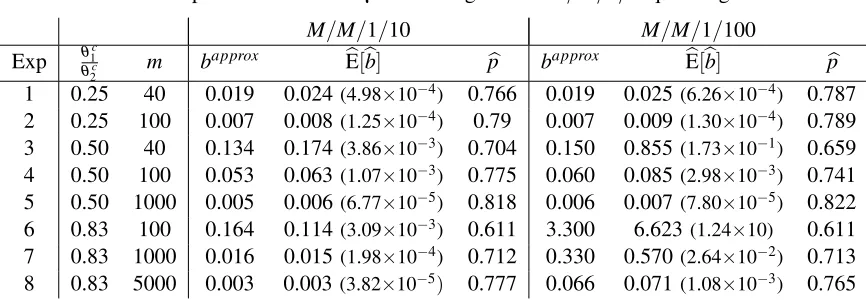
Table 1: How power holds whenγ=bapprox given a truly quadratic response function. θ₁c θ₂c r m bapprox(=γ) bE[bb] Varc[bb] p_b

5 2 1000 40 0.2125 0.2111 4.52×10−3 0.79

To show our diagnostic test has this desired power we run a macro-experiment, repeating the diagnostic testG=1000 times. An estimate of power will be given by the proportion of times the null hypothesis is rejected; we denote this estimate p_b. In Table 1 p_bis recorded along with Eb[bb] andVarc[bb], the sample

mean and variance of the bias estimates recorded over the G=1000 macro-replications. Also reported is

bapprox, the true bias in this quadratic example, which we set equal toγ, the relevant bias.

To complete the diagnostic test we use the methods presented in §3.1 to §3.3. Given true input parametersθ₁c=5 andθ₂c=2 withξ₁2=2 andξ₂2=1.5,m=40 observations ofX1andX2were generated

from the bivariate normal distribution and used to estimate the MLEs,θθθmle, and Ωb. We set the number

of replications to r=1000 then built a response surface model using a CCD centred atθθθmle with width

set usinga=0.283 selected to ensure a power of 1−α2=0.8. In each replication we ran the simulation

by adding N (0,0.01) noise to (10). Given the response surface model the bias estimator, bb, and its

variance, Var(bb), could be evaluated enabling the calculation of the test statistic, T, and the conclusion of

the diagnostic test. This process was repeated G=1000 times to gain the results shown in Table 1. In Table 1 we see that when the response function is truly quadratic, the diagnostic test holds power very close to 1−α2=0.8 as desired. We also see that the average of the bias estimates,bE[bb], is very close

to the true bias.

We will now investigate how well the diagnostic test performs when the quadratic assumption does not hold, by studying a tractableM/M/1/C queueing model.

4.2 M/M/1/C Queueing Model

Consider an M/M/1/C queueing model with true arrival rate θ₁c, service rateθ₂c and finite capacity C.

Here inter-arrival times of customers,Ai, follow an exponential distributionAi∼Exp(θ₁c), as do the service

times, Si∼Exp(θ₂c), for i=1,2, . . . ,m observations. For this queueing model the expected number of

customers in the system, E[Y|θθθ], can be expressed in closed form

η(θθθ) =E[Y|θθθ] = θ1 θ2−θ1

−(C+1)θ C+1 1 θ₂C+1−θ₁C+1

. (11)

It is therefore possible to derive the second-order partial derivatives yielding H(θθθc); this allows the evaluation

ofbapprox, the delta method approximation of bias.

We shall now, for the purpose of the experiment, assume that the true response function, Equation (11), is unknown. We want to evaluate the quality of our diagnostic test for detecting a relevant bias when the response function is not truly quadratic. To do this we will look at both theM/M/1/10 andM/M/1/100 queueing models over a number of parameter settings to see how well the power, set at 1−α2=0.8, holds

when relevant bias, γ, is set equal to the delta approximation of bias bapprox. As before, to measure the

power we record the proportion of times the null hypothesis was rejected overG=1000 macro-replications of the diagnostic test, bp. The results of the experiments are given in Table 2.

The diagnostic test was completed as follows. Instead of running a nominal experiment we used the true input distributions to generatemobservations from the arrival and service distributions,Ai,Si for i=1,2, . . . ,m, then estimated the MLEs,θθθmle, and the covariance matrix,Ωb; we know that Cov(θ₁mle,θ₂mle) =

0. Also, rather than directly simulating the M/M/1/C queue we add N(0,0.05) noise to (11) for each replication. The number of replications to be run at each design point was set to r=500 allowing the identification of the value of a required for the power to hold at 1−α2=0.8. A CCD design, centred

Table 2: How power holds whenγ=bapprox given an M/M/1/C queueing model.

M/M/1/10 M/M/1/100

Exp θ1c

θ₂c m b

approx

b

E[bb] p_b bapprox bE[bb] _bp

1 0.25 40 0.019 0.024 (4.98×10−4_{) 0.766 0.019 0.025(6.26×10}−4_{) 0.787}

2 0.25 100 0.007 0.008 (1.25×10−4) 0.79 0.007 0.009(1.30×10−4) 0.789 3 0.50 40 0.134 0.174 (3.86×10−3) 0.704 0.150 0.855(1.73×10−1) 0.659 4 0.50 100 0.053 0.063 (1.07×10−3_{) 0.775 0.060 0.085(2.98×10}−3_{) 0.741}

5 0.50 1000 0.005 0.006 (6.77×10−5) 0.818 0.006 0.007(7.80×10−5) 0.822

6 0.83 100 0.164 0.114 (3.09×10−3) 0.611 3.300 6.623(1.24×10) 0.611

7 0.83 1000 0.016 0.015 (1.98×10−4) 0.712 0.330 0.570(2.64×10−2) 0.713 8 0.83 5000 0.003 0.003(3.82×10−5) 0.777 0.066 0.071(1.08×10−3) 0.765

were run at each design point and the response surface fitted allowing evaluation ofHb(θθθmle), the estimated

Hessian matrix. We were therefore able to estimate the delta approximation of bias, bb, and its variance,

Var[bb], allowing us to calculate the test statistic and conclude the hypothesis test. This process was repeated overG=1000 macro-replications giving pbandbE[bb], the average of the bias estimates, both are recorded

in Table 2.

In Table 2, we see that across all experiments, whetherC=10 or 100, as the amount of input data is increased bpgets closer to the desired power 1−α2=0.8 and the average bias estimateEb[bb]gets closer to

the delta approximationbapprox. Both parameter estimates improve due to the the increase in information which seesθθθmle get closer toθθθc, the true input parameters. This is important in our method as, ideally,

we would centre our CCD atθθθc to find the curvature of the response function at that point, H(θθθc).

Experiments 6, 7 and 8 look at the system under high traffic intensity,ρ=θ₁c/θ₂c=0.833. In Experiment

6, where m=40, we saw a reasonably high proportion of instances (≈10%) where the estimated traffic intensity exceeded 1, i.e. ρ=θ₁mle/θ₂mle>1. When this occurs the number of people in the queue will

increase up to capacity and remain around that level. The behaviour of the response surface in these cases is not quadratic and therefore the delta method does not perform well which is reflected in the average bias estimate, bE[bb], and power, ˆp. One way to fix this problem is to collect more data, m, until θ₁mle/θ₂mle<1 consistently, as we did in Experiments 7 and 8 where the bias estimate bE[bb]gets closer to

the delta approximation.

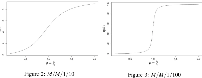
This problem is not unique to bias estimation: it will occur in any simulation model with finite capacity and traffic intensity close to 1. If the amount of data available is small and we cannot accurately estimate the input parameters it is easy to conclude that a system will become saturated when in reality it might not. In experiments 6, 7 and 8, where a high traffic intensity was investigated, we see the effect of the shape of the true response surface on how well the power holds. The shape of the response surface is driven by the capacity, C. This directly links to how closelyθθθc can be estimated byθθθmle. In Figure 3 we see that

for theM/M/1/100 queue, with higher capacity, there is a more dramatic change in the response surface for small changes of θ1 and θ2 than there is for the lower capacity, M/M/1/10, queue seen in Figure 2.

Close toρ= 1, where the response surface changes more dramatically, more observations,m, are needed to

ensure we are estimating the Hessian, H(θθθc), close enough toθθθcto capture the true curvature at that point.

This could also be affected by the variability of the MLEs; when the variance is large even if we haveθθθmle

close toθθθcon average, we could see large variability in the response from replication to replication. In the

higher capacity system small changes in the inputs have a larger effect on the simulation output which is used to fit the response surface and therefore estimate the Hessian. For the lower capacity queueing model the distance betweenθθθmle andθθθc has a less pronounced effect on the simulation response as the response

Figure 2: M/M/1/10 Figure 3: M/M/1/100

We also note that for the M/M/1/100 queueing model, in Experiments 3, 6 and 7 pbis lower than

the desired power of 0.8 but the average of the bias estimates in these cases, bE[bb], is higher than bapprox.

Intuitively, this seems contradictory as we would expect to reject the null hypothesis more often if bias is much more extreme thanγ=bapprox. In these cases we also seebE[bb]has large standard error. Investigating

the test statistics over theG=1000 macro replications, using Q-Q plots, illustrated that these were the cases where the distribution of the test statistics was far from the assumed normal distribution. In Experiments 4, 5 and 8 given more input data the normality assumption held much better. For theM/M/1/10 queueing model the normality assumption held well in all cases. This again illustrates the importance of centring the CCD close toθθθc, especially when there is a sharp change in the shape of the response surface.

As an aside we also considered the trade off between the variables a and r, used to set the width of the experimental design. To improve the quadratic assumption it is tempting to shrinka and increase the number of replications at each design point to ensure the power still holds. This is very expensive computationally; to halvea, and thus the width of the design, in the experiments above we would have had to increase the number of replications at each design point tor=8000. Looking at the experiments above we saw little improvement on the estimated power _bpfrom halvinga. This is because shrinking the width of the design would only be helpful if the CCD was centred very close toθθθc; no amount of computational

effort will improve our estimate ofHb(θθθmle) if the design is centred atθθθmle far fromθθθc.

4.3 A Realistic Example - NHS 111 Healthcare Call Centre

We will now illustrate our bias detection diagnostic on the simulation of a real-world system with a non-stationary input process. The nominal experiment is based on observations of an NHS111 healthcare call centre simulated using anM(t)/G/S(t)queueing model with a piecewise-constant Poisson arrival process. Using the methods discussed by Morgan et al. (2016) we were able to quantify the total IU about the expected waiting time of callers, E(WTime). The system discussed is staffed to meet the NHS target level of service, P(Wait > 1 min)<0.05; in the nominal experiment an estimate of the expected waiting time of customers was found to be E(WTime) =0.0674 minutes. In the following tests we use the value of IU, defined to be Var[η(θθθmle)], to guide our choice ofγ. Let γ=

√

υ×IU where 0<υ <1. This gives us

the threshold bias thought to have an important effect on the MSE. Estimates ofθθθc,Ωandσ2, given by θθθmle,Ωb andσ_b2, were collected within the nominal experiment. In practice the estimate of the simulation

estimation error,σb

2_{, could have been used here to aid the choice ofr, the number of replications at each}

design point. For example, if we had a noisy simulation a large value of r would be required. In the following experimentsr=500 replications were performed at each design point.

Given observations of the NHS111 healthcare call centre system we conducted two experiments with different levels of input data. We denote by m1 the number of days of observations of the arrival process

Table 3: Results of the bias detection test for an NHS 111 healthcare call centre when considering expected waiting time of callers, E(WTime).

Exp m1 m2 IU(Var[η(θθθc)]) γ (υ=0.3) bb Var[bb] p-value

1 10 20068 4.336×10−5 _3.61×10−3 _6.03×10−3 _1.638−6 _1.23×10−6

2 26 52711 1.907×10−5 2.39×10−3 4.04×10−3 7.215×10−7 9.97×10−7

size toα1=0.05. For these experiments the relevant bias,γ, was set usingυ=0.3, meaning we consider

bias squared higher than 0.3 times the value of IU to be concerning.

From Table 3 we see that in Experiment 1, where we considered a smaller number of observations of the arrival process,m1=10 days, we have sufficient evidence to reject the null hypothesis as the p-value is

less thanα1=0.05. We can therefore conclude that the amount of bias due to input modelling about the

expected waiting time of callers, E(WTime), is significant. In addition, using the output of the diagnostic

test we can calculate a confidence interval about our estimate of bias asbb±Z₁−α1

q

Var(bb). This allows us to make a statement about howbbcompares to the relevant bias γ. In Experiment 1 a 90% confidence

interval aboutbb is given by (3.92×10−3,8.14×10−3). This does not contain γ, the relevant bias, and we

can therefore conclude at the 90% significance level that bias due to input modelling is more than γ in

this system. In Experiment 2 we observedm1=26 days of observations of the arrival process which saw

a reduction in IU and therefore γ, but again we were able to reject the null. A 90% confidence interval

aboutbbis given by (2.64×10−3,5.44×10−3) which again does not containγ. In both cases the practitioner

can be confident that the level of bias due to input modelling is high enough for them to be concerned. When the bias is relevant, as is the case here, it should be taken into account in assessing the total uncertainty about the simulation output due to input modelling. This will allow more informed decisions to be made. At this point it could be considered sensible to spend more computational effort running the delta approximation alone to obtain a more accurate estimate of the bias due to input modelling.

The practitioner may, alternatively, wish to reduce bias to a level that does not concern them by collecting more input data. Changing the number of intervals describing the piecewise-constant Poisson arrival process may also have an affect on the bias due to input modelling. Morgan et al. (2016) used change point analysis as a pre-processing step in their IU quantification method. This aided the choice of arrival intervals but did not guarantee an arrival function that represented the true arrival process well or that had minimal error due to input modelling. Our method now provides the bias estimate needed to be able to compare two arrival functions in terms of the MSE due to input modelling.

5 CONCLUSION

This paper presents a diagnostic test with controlled power of detecting bias due to input modelling of a relevant size in simulation models.

Within the diagnostic test the experimental design is centred atθθθmleour best estimate of the true input

parameters,θθθc. When the response surface, at the pointθθθc, is sensitive to the input parameters we found

more input data was required to estimate the delta approximation of bias well and retain the desired power. Although the problem here seems to be the discrepancy betweenθθθmleandθθθc it could be that the quadratic

assumption is not satisfactory; this assumption is always approximate with small samples, in which case a higher-order approximation should be used.

parameters our method is a good step forward to being able to detect when bias due to input modelling is of a concerning size.

REFERENCES

Cheng, R. C., and W. Holland. 1997. “Sensitivity of Computer Simulation Experiments to Errors in Input Data”.Journal of Statistical Computation and Simulation57 (1-4): 219–241.

Dean, A., and D. Voss. 1999.Response Surface Methodology. Springer-Verlag, New York.

Liu, W. 1997. “On some sample size formulae for controlling both size and power in clinical trials”.Journal of the Royal Statistical Society: Series D (The Statistician)46 (2): 238–251.

Montgomery, D. C. 2013.Design and Analysis of Experiments. John Wiley & Sons.

Morgan, L. E., A. C. Titman, D. J. Worthington, and B. L. Nelson. 2016. “Input uncertainty quantification for simulation models with piecewise-constant non-stationary Poisson arrival processes”. In Proceedings of the 2016 Winter Simulation Conference, edited by T. Roeder, P. I. Frazier, R. Szechtman, E. Zhou, T. Huschka, and S. E. Chick, 370–381. Piscataway, New Jersey: Institute of Electrical and Electronics Engineers, Inc.

Nelson, B. 2013.Foundations and Methods of Stochastic Simulation: A First Course. Springer Science & Business Media.

Song, E., and B. L. Nelson. 2015. “Quickly Assessing Contributions to Input Uncertainty”. IIE Transac-tions47:893–909.

Withers, C. S. 1987. “Bias Reduction by Taylor Series”.Communications in Statistics-Theory and Methods16 (8): 2369–2383.

Withers, C. S., and S. Nadarajah. 2014. “Bias Reduction: The Delta Method versus the Jackknife and the Bootstrap.”.Pakistan Journal of Statistics30 (1): 143–151.

ACKNOWLEDGEMENTS

We gratefully acknowledge the support of the EPSRC funded EP/L015692/1 STOR-i Centre for Doctoral Training, NSF Grant CMMI-1068473 and GOALI sponsor Simio LLC. We also thank Bruce Ankenman for insightful discussion and suggestions.

AUTHOR BIOGRAPHIES

LUCY E. MORGAN is a Ph.D. student of the Statistics and Operational Research Centre for Doctoral Training in Partnership with Industry at Lancaster University. Her research interests are input uncertainty in simulation models and arrival process modelling. Her email address is [email protected].

BARRY L. NELSONis the Walter P. Murphy Professor in the Department of Industrial Engineering and Management Sciences at Northwestern University and a Distinguished Visiting Scholar in the Lancaster University Management School. He is a Fellow of INFORMS and IIE. His research centers on the design and analysis of computer simulation experiments on models of stochastic systems. His e-mail address is

[email protected].

ANDREW C. TITMAN received his Ph.D. from University of Cambridge and currently is Lecturer in Statistics in the Department of Mathematics and Statistics at Lancaster University. His research interests include survival and event history analysis and latent variable modeling, with applications in biostatistics and health economics. His email address [email protected].