Daniel Gildea
∗ University of RochesterGiorgio Satta
∗∗ Universit`a di PadovaXiaochang Peng
† University of RochesterMotivated by the task of semantic parsing, we describe a transition system that generalizes standard transition-based dependency parsing techniques to generate a graph rather than a tree. Our system includes a cache with fixed sizem, and we characterize the relationship between the parametermand the class of graphs that can be produced through the graph-theoretic concept of tree decomposition. We find empirically that small cache sizes cover a high percentage of sentences in existing semantic corpora.
1. Introduction
As statistical natural language processing systems have progressed to provide deeper representations, there has been renewed interest in graph-based representations of se-mantic structures and in algorithms to produce them. Typically, these algorithms behave similarly to standard parsing algorithms for retrieving syntactic representations: They take as input a sentence and produce as output a graph representation of the semantics of the sentence itself.
At the same time, recent years have seen a general trend from chart-based syntactic parsers toward stack-based transition systems, as the accuracy of transition systems has increased, and as speed has become increasingly important for real-world applications. On the syntactic side, stack-based transition systems for projective dependency parsing run in time O(n), where n is the sentence length; for a general overview of these systems, see, for instance, the presentation of Nivre (2008). There have also been
∗Computer Science Department, University of Rochester, Rochester NY 14627. E-mail:[email protected].
∗∗Dipartimento di Ingegneria dell’Informazione, Universit`a di Padova, Via Gradenigo 6/A, 35131 Padova, Italy. E-mail:[email protected].
†Computer Science Department, University of Rochester, Rochester NY 14627. E-mail:[email protected]
Submission received: 19 December 2016; revised version received: 26 June 2017; accepted for publication: 7 July 2017.
a number of extensions of stack-based transition systems to handle non-projective trees (e.g., Attardi 2006; Nivre 2009; Choi and McCallum 2013; G ´omez-Rodr´ıguez and Nivre 2013; Pitler and McDonald 2015).
Stack-based transition systems can produce general graphs rather than trees. Per-haps the simplest way to generate graphs is to shift one word at a time onto the stack, and then consider building all possible arcs between each word on the stack and the next word in the buffer. This is essentially the algorithm of Covington (2001), generalized to produce graphs rather than non-projective trees. This algorithm was also cast as a stack-based transition system by Nivre (2008). The algorithm runs in time O(n2), and requires the system to discriminate the arcs to be built from a large set of possibilities, potentially leading to errors.
Traditional stack-based parsing, which is restricted to trees, and the Covington algorithm as generalized to graph parsing can be thought of as two extremes, with a wide set of possible intermediate approaches staking out different trade-offs between expressiveness, on the one hand, and time and the discrimination required of machine learning components on the other. In this article, we mathematically explore this trade-off and precisely characterize the relationship between parsing systems and the set of graphs they can build. We describe a parsing system based on adding a working set, which we refer to as a cache, to the traditional stack and buffer. With cache size 2, our algorithm can only build trees, while with unbounded cache, our algorithm can build any graph, because it is then equivalent to the Covington algorithm generalized to graphs. We speculate that small, fixed cache sizes provide a good trade-off for fast and accurate string-to-graph parsing.
We analyze the class of graphs that can be successfully constructed by our parsing system, making use of the graph-theoretic notion of treewidth. The treewidth of a graph gives a measure of how tightly interconnected it is: Trees have treewidth 1, and fully connected graphs onnvertices have treewidthn−1. We show that the class of graphs constructed by our parser is precisely characterized by treewidth: A transition system of cache size mcan produce graphs of treewidth m−1. Our framework assumes an input order of vertices, corresponding to the word order of the string, and we define a concept of relative treewidth to characterize the set of graphs that the parser can produce given a fixed input order of vertices. Finally, we develop an oracle algorithm for our parsing system, and prove its correctness. We also provide an algorithm for computing the minimal cache size needed to parse a given data set.
proposed (Kuhlmann and Oepen 2016), we also experiment with three sets of semantic dependencies from the Semeval 2015 semantic dependency parsing task (Oepen et al. 2015). With these data sets, which are generally closer to the surface string structure than Abstract Meaning Representation, we find somewhat higher relative treewidth. In every data set that we analyzed, over 99% of sentences can be covered with a cache size of eight.
2. Tree Decomposition and Treewidth
In this section we introduce and define the notions of tree decomposition and treewidth, as well as a few related concepts that we will use throughout this article. As usual, we denote an undirected graph asG=(V,E), where Vis the set of vertices andE is the set of edges. Each edge is represented as an unordered pair (u,v) withu,v∈V.
The theory developed in this article is based on the graph theoretical notion of tree decomposition, which has been independently developed in several areas of computer science and discrete mathematics. From an application-oriented perspective, tree decomposition has proven very useful in discrete optimization and in the design of polynomial time algorithms using dynamic programming techniques.
The intuitive idea behind the notion of tree decomposition can be explained as follows. At this point, we use the term “interconnection” in a rather informal way; the precise meaning of this notion will be mathematically defined later. A tree is a special kind of graph where the vertices are arranged in a hierarchical way, with the property that the set of vertices in any subtree have only one interconnection with the set of the remaining vertices. In contrast, for a general graph this is not pos-sible, meaning that we cannot group vertices in a hierarchical structure and pretend that there are a small number of interconnections between vertices in any subtree and the remaining vertices. This is apparent for a complete graph, that is, a graph where each vertex is connected with every other vertex. More interestingly, this is also true for a grid-like graph, where any hierarchical decomposition of the set of vertices will always lead to some subtree with a number of interconnections with the remaining structure that is not bounded by a constant. Note that, in contrast with a complete graph, where each vertex has a number of neighbors that is not bounded by a constant, in a grid each vertex has at most four neighbors. Still, the internal structure of a grid is unfavorable for this type of hierarchical arrangement. The no-tion of tree decomposino-tion of a graph, and the related nono-tion of treewidth, provide us precisely with the information we need: To what degree is it possible to arrange the vertices of a graph into some hierarchical structure, with the property that inter-connections between vertices in any subtree and the remaining vertices are kept to a minimum?
is defined as a pair ({Xi|i∈I},T=(I,F)) where tree T satisfies all of the following
properties.
r
Vertex cover:The nodes of the treeTcover all the vertices ofG:Si∈IXi=V.
r
Edge cover:Each edge inGis included in some node ofT. That is, for alledges (u,v)∈E, there exists ani∈Iwithu,v∈Xi.
r
Running intersection:The nodes ofTcontaining a given vertex ofGform aconnected subtree. Mathematically, for alli,j,k∈I, ifjis on the (unique) path fromitokinT, thenXiTXk⊆Xj.
Thewidthof a tree decomposition ({Xi},T) is maxi|Xi| −1. Thetreewidthof a graph
is the minimum width over all tree decompositions
tw(G)= min ({Xi},T)∈TD(G)
max
i |Xi| −1
where TD(G) is the set of valid tree decompositions of G. We refer to a tree decom-position achieving the minimum possible width as beingoptimal.
In general, more densely interconnected graphs have higher treewidth. For in-stance, any tree has treewidth 1, a graph consisting of a single cycle with three or more vertices has treewidth 2, and a fully connected graph ofnvertices has treewidth
n−1. Low treewidth thus indicates some treelike structure underlying the graph. When certain properties of the graph must be checked, the tree decomposition is often helpful in organizing computation (see, e.g., results of Courcelle [1990] and Arnborg, Lagergren, and Seese [1991]). Finding the treewidth of a graph is an NP-complete problem (Arnborg, Corneil, and Proskurowski 1987).
Example 1
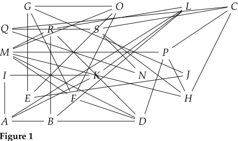
Consider the graphGin Figure 1 with vertex setV={A,B,C,. . .,Q,R,S}. At first sight,
G’s structure seems rather intricate, with edges scattered all over the picture. However, an optimal tree decomposition ofGreveals that there is a tree-like structure underlying
G. An optimal tree decompositionTofGis displayed in Figure 2(a), where we use gray
A B
C
D
E F
G
H
I K J
L
M
N O
P
[image:4.486.50.285.509.648.2]Q R S
Figure 1
I A B D F G J
K L R M O E
P
C
Q H
S
N
(a)
ALB LBR BRD RDM DMF MFO FOG
KAL DMP OGE
IKA MPH GEJ
PHC
HCS CSQ SQN
[image:5.486.53.426.67.239.2](b)
Figure 2
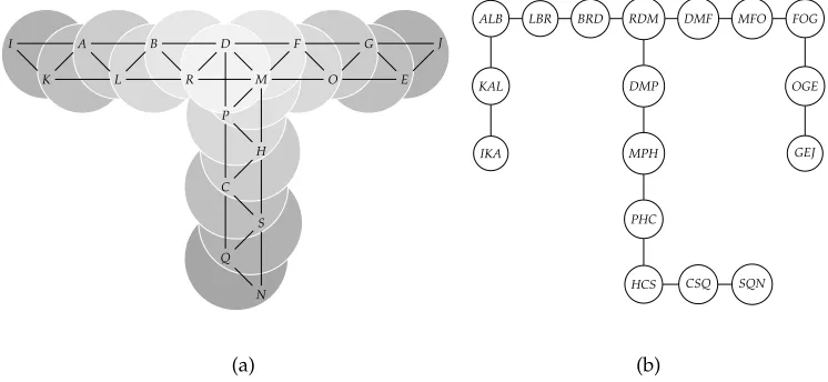
(a) An optimal tree decomposition of graphGin Figure 1; this is a set of overlapping clusters of
G’s vertices, arranged in a tree. (b) The high-level treelike structure ofGbecomes apparent when it is drawn ignoringG’s edges.
circles to indicate the sets of vertices ofGthat represent the bags ofT. Because adjacent bags ofTshare some of their vertices, our gray circles partially overlap. The tree-like structure underlyingGis apparent from this overlapping. This tree decomposition has bags of three vertices each, and thus the graph’s treewidth is 2. In this representation, it is also apparent that there is a low number of interconnections among vertices in a subtree ofTand the remaining vertices ofG.
An alternative representation of the same tree decomposition is shown in Fig-ure 2(b), where we focus on the vertices and ignore the edges of the graph. It is easy to see that the vertex cover and the edge cover conditions in the definition of tree de-composition are both satisfied byT. As an example of the running intersection property, note that the vertexSappears in three adjacent nodes of the tree decomposition.
Although general tree decompositions are undirected trees, in this article we will work with rooted, directed tree decompositions, in which one node is designated as the root, and the children of each node are ordered. We say that a rooted, ordered tree decomposition of graphGhaving widthkissmoothif each bag contains exactlyk+1 vertices, and each bag contains the same vertices as its parent bag, with exactly one vertex removed and one vertex added. The tree decomposition in Figure 2(b) is smooth. The concept of smooth tree decompositions, for standard unrooted tree decompo-sitions, was introduced by Bodlaender (1996). Throughout this article, we also require that the root of a smooth tree decomposition containsk+1 copies of the special symbol $, with vertices ofGbeing added one at a time in the bags below the root. It is easy to see that the size of a smooth tree decomposition (i.e., the number of nodes of the tree) is the number of vertices in the graph plus one.
Lemma 1
Proof.Letkbe the width ofT. At each bag having fewer thank+1 vertices, continue adding vertices from adjacent bags until all bags have the same size. If two adjacent bagsB1andB2end up having the same vertices, collapseB1andB2into a single bag, and merge the children of the two bags in a way that preserves their order. If two adjacent bagsB1andB2differ by more than one vertex in their contents, add intermediate bags by adding vertices fromB2and removing vertices fromB1one at a time. Finally, choose a bagBas the root of the tree constructed so far. Add a new root containingk+1 instances of the special symbol $, and intermediate bags connecting the root to B adding one vertex ofBat a time, and removing instances of $. As already discussed in the Introduction, in natural language processing applica-tions, we are not provided with a graph structure as input, and we are not asked to recognize whether that graph belongs to some formal language. We are instead given as input an ordered sequence of vertices of some graph, or a superset thereof, and we are asked to retrieve the graph itself. Although this latter problem is apparently more difficult than the former, since the edges of the graph must be decoded, the input ordering of the vertices plays an important role and can be used to restrict the search space, ultimately ending up with a more efficient computation. This idea is at the basis of the algorithms for graph parsing developed in this article. We therefore now introduce the notion of relative treewidth with respect to a given order of the vertices of a graph, which is original to this article.
LetG=(V,E) be some graph and letT be a smooth tree decomposition ofG. We define the vertex orderπ(T) ofT to be the sequence of vertices produced by visiting
T in a preorder, left to right traversal and by listing the vertices newly introduced at the visited bags. Each vertex of V will appear exactly once in π(T). We will analyze the behavior of our parser when given a fixed input order over the vertices in terms of a notion of relative treewidth with respect to the input order. We define the relative treewidthofGwith respect to an orderπofG’s vertices to be the minimum width of any tree decomposition ofGwhose vertex order isπ. Formally, we write
rtw(G,π)= min ({Xi},T)∈TD(G),
π(T)=π
max
i |Xi| −1.
Example 2
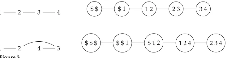
Consider the chain-like graphGin Figure 3, with vertex set{1, 2, 3, 4}. In the top row,
Gis presented in vertex order π=(1, 2, 3, 4), along with a tree decompositionTsuch that π(T)=π. In the bottom rowG is presented in vertex orderπ0=(1, 2, 4, 3), with the tree decompositionT0achieving the minimum width such thatπ(T0)=π0. The order
π0increases the relative treewidth:rtw(G,π)=1, whilertw(G,π0)=2.
We note that, for any graphG, there exists a vertex order achieving its optimal width tw(G)=min
π rtw(G,π)
1 2 3 4 $ $ $ 1 1 2 2 3 3 4
[image:7.486.55.422.65.159.2]1 2 4 3 $ $ $ $ $ 1 $ 1 2 1 2 4 2 3 4
Figure 3
A chain-like graphG, presented at top left in vertex orderπ=(1, 2, 3, 4) and at bottom left in vertex orderπ0=(1, 2, 4, 3). Tree decompositions with minimum relative treewidth with respect toπandπ0are displayed at the right. We havertw(G,π)=1 andrtw(G,π0)=2.
Although our notion of relative treewidth with respect to a vertex order is super-ficially similar to the standard vertex elimination algorithm for finding a tree decom-position (Bodlaender 2006), which also takes as input a vertex order, these orders are in fact distinct. We will not make use of the vertex elimination algorithm in this article, but we describe it briefly here for readers interested in the connection between these two concepts. In the vertex elimination algorithm, vertices are processed in the input order, by adding edges connecting the current vertex’s remaining neighbors and then eliminating the current vertex. Each vertex along with its neighbors at the time of its elimination form one bag of the tree decomposition. The order of the vertex elimination algorithm corresponds to the order in which vertices are introduced in some outside–in traversal of the tree decomposition, whereas the order of our concept of relative treewidth corresponds to a pre-order traversal of a smooth tree decomposition.
3. Cache Transition Parser
In this section, we introduce a nondeterministic computational model for graph-based parsing, which we call acache transition parser. The model takes as input an ordered sequence of vertices, reads it strictly from left to right, and incrementally produces a graph as output. Our model is an extension of the transition-based parsing framework described by Nivre (2008) for dependency tree parsing. We assume the reader is familiar with such a framework. We also provide a characterization of our cache transition parsers using the notions of tree decomposition and width that have been introduced in Section 2. Throughout this section, for integerm≥1 we write [m] to denote the set
{1,. . .,m}.
Because the cache has fixed size, in order to be able to read a new vertex from the buffer and shift it into the cache, we need to make new room in the cache by moving some other vertexvfrom the cache into the stack. Oncevis in the stack, it is no longer accessible for the operations of edge construction. Typically, the parser movesvout of the cache and into the stack when it predicts that, in the process of edge construction,
vdoes not need to be accessed for a while. For instance, this happens whenv’s neighbors that still need to be processed are all placed at a far distance in the buffer.
Crucially, the cache is not governed by a first-in first-out policy as in a queue: The vertexvthat we move out of the cache might not be the “oldest” vertex that has been introduced in the cache itself. As a consequence, the choice of the vertex that is moved out of the cache and into the stack at each step may considerably alter the original ordering of the vertices in the input.
In addition to this operation, it is also possible to pop some vertex from the stack and put it back into the cache. Again, because the cache has fixed size, in order to be able to do this we need to make new room in the cache. This time this is done by permanently removing some vertex from the cache, meaning that this vertex is dropped out of the parser storage. This happens when the parser decides that all of the edges impinging on a vertex have been processed, and the vertex itself is no longer needed. Going back to our running example about vertex v, when the far distance neighbors of v will reach the foremost position of the buffer and will be shifted into the cache, we can exploit the previous operation, popvfrom the stack, and move it back into the cache, where it will be available for the construction of the new edges. Altogether, the combination of these two operations has the effect of repeatedly moving v back and forth between the cache and the stack.
Formally, acache transition parserconsists of a stack, a cache, and an input buffer. The stack is a sequence σ of vertices and integers, as explained subsequently, with the topmost element always at the rightmost position. The buffer is a sequence of verticesβcontaining a suffix of the input, with the first element to be read at the leftmost position. Finally, the cache is a sequence of vertices η. The element at the leftmost position is called the first element of the cache, and the element at the rightmost position is called the last element.
Operationally, the functioning of the parser can be described in terms of configu-rations and two transitions. Each transition is a binary relation defined on the set of configurations. Aconfigurationof our parser has the form:
c=(σ,η,β,E)
where σ,η, and βare as described earlier, andE is the set of edges being built. The initial configuration of the parser is ([], [$,. . ., $], [v1,. . .,vn],∅), meaning that the stack
and edge set are initially empty, and the cache is filled withmoccurrences of the special symbol $. The final configuration is ([], [$,. . ., $], [],EG), where the stack and the cache
Thetransitionsof the parser are specified as follows.
r
push(i,C) is parameterized by a position in the cachei∈[m] and a set of positions in the cacheC⊆[m]\ {i}. It takes a configuration:(σ, [v1,. . .,vi−1,vi,vi+1,. . .,vm],v|β,E)
and moves to a configuration:
(σ|i|vi, [v1,. . .,vi−1,vi+1,. . .,vm,v],β,E0)
E0=E∪ {(vk,v) | k∈C}
Here, we have shifted the next vertexvout of the buffer and moved it into the last position of the cache. We have also taken the vertexviappearing
in positioniin the cache and pushed it onto the stackσ, along with the integerirecording the position in the cache from which it came. Finally, we have added some edges to the graph being built, where the new edges connect the shifted vertexvwith some subset of the other vertices in the cache. This subset is specified by the parameterC.
r
poptakes a configuration:(σ|i|v, [v1,. . .,vm],β,E)
and moves to a configuration:
(σ, [v1,. . .,vi−1,v,vi,. . .,vm−1],β,E)
Here we have popped a vertexvfrom the stack, along with the integeri
recording the position in the cache that it originally came from. We placev
in positioniin the cache, shifting the remainder of the cache one position to the right, and discarding the last element in the cache.
Example 3
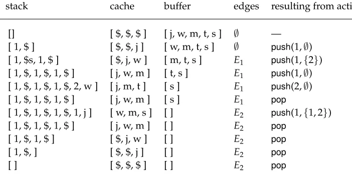
Consider the sentence “John wants Mary to succeed” and the associated semantic representation displayed as a graph in Figure 4. Note that the graph, with vertices in the order of the English sentence, corresponds to the graph at the bottom row of Figure 3. When given the vertex sequence [j, w, m, t, s] as input, our nondeterministic parser will be able to construct the given graph using the run displayed in Figure 5. For instance, when the parser reaches the configuration ([1, $, 1, $, 1, $], [j, w, m], [s],
w
j s
m
Figure 4
Graph for the semantic representation of the sentence “John wants Mary to succeed.” Vertex w represents word tokenwants, vertex j representsJohn, vertex s representssucceed, and vertexm
representsMary.
We have described our transition system as producing undirected graphs with unlabeled edges, but it can be easily extended to produce directed graphs and labeled edges. Directed graphs can be produced by modifying the parameter C of the push transition to be defined as a set of tuples, where each tuple consists of an integerkand a binary variable that specifies whether to produce edge (v,vk) or edge (vk,v). Similarly,
labeled edges can be produced by adding a value to each tuple specifying the edge’s label. Notice that the tuple representation could also be used to allow multiple arcs between the same two nodes, with different directions and labels. These extensions do not fundamentally change the set of graphs that can be produced with a given cache size; a directed (or labeled) graph can be produced if and only if its undirected (or unlabeled) counterpart can be produced. For this reason, we treat our graphs as undirected (and unlabeled) in the remainder of this article.
We now show that, in our parser, each pop transition reverses the effect of some previous push transition, in a sense that will be specified below. For s≥1, consider a
stack cache buffer edges resulting from action
[image:10.486.50.401.451.628.2][] [ $, $, $ ] [ j, w, m, t, s ] ∅ — [ 1, $ ] [ $, $, j ] [ w, m, t, s ] ∅ push(1,∅) [ 1, $s, 1, $ ] [ $, j, w ] [ m, t, s ] E1 push(1,{2}) [ 1, $, 1, $, 1, $ ] [ j, w, m ] [ t, s ] E1 push(1,∅) [ 1, $, 1, $, 1, $, 2, w ] [ j, m, t ] [ s ] E1 push(2,∅) [ 1, $, 1, $, 1, $ ] [ j, w, m ] [ s ] E1 pop
[ 1, $, 1, $, 1, $, 1, j ] [ w, m, s ] [ ] E2 push(1,{1, 2}) [ 1, $, 1, $, 1, $ ] [ j, w, m ] [ ] E2 pop
[ 1, $, 1, $ ] [ $, j, w ] [ ] E2 pop
[ 1, $, ] [ $, $, j ] [ ] E2 pop
[ ] [ $, $, $ ] [ ] E2 pop
Figure 5
Example run of the cache transition system constructing the graph of Figure 4. We have set
sequence of 2stransitionsγ=t1,. . .,t2s. We say thatγisminimal reversingif it consists
ofspush transitions intermixed withspop transitions, with the property that in any proper prefix ofγof the formt1,. . .,tk,k∈[2s−1], the number of push transitions is
strictly greater than the number of pop transitions. It is not difficult to see that, ifγis minimal reversing,t1must be a push transition andt2smust be a pop transition.
Lemma 2
Letcbe a configuration of the parser with stackσand cacheη. Let alsoγbe a minimal reversing sequence of transitions. If we apply tocthe transitions ofγin the given order, we reach a configurationc0with stackσ0=σand cacheη0=η.
Proof.Let γ=t1,. . .,t2s. We proceed by induction ons. Ifs=1,γ must be composed
by a push followed by a pop. The definition of the pop transition exactly restores the stack and the cache of the configurationcto which the push applied.
Ifs>1, letγ0=t2,. . .,t2s−1. It is not difficult to see thatt2must be a push transition and t2s−1 must be a pop transition. However, a proper prefix of γ0 might now have a number of push transitions that equals the number of pop transitions, making γ0
not minimal reversing. If this is the case, we splitγ0 exactly at that point, and apply the same reasoning to the two subsequences, until γ0 is divided into subsequences that are all minimal reversing. Assume now thatc1 is the configuration obtained by applying t1 toc, andc2s−1 is the configuration obtained by applyingγ0 toc1. Using the inductive hypothesis on each of the minimal reversing subsequences of γ0, we obtain that the stack and the cache of c1 and c2s−1 are equal. We have already observed that a pop transition applied toc1 would restore the stack and the cache of c. Because the stack and the cache ofc1 andc2s−1 are the same, we conclude that the pop transition t2s applied to c2s−1 produces configuration c2s with exactly the same
stack and cache asc.
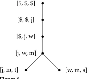
Consider now a complete run of the parser, that is, a run starting at the initial configuration for a given input, and ending in a final configuration. Lemma 2 suggests that such run can be represented by means of some underlying tree structure, as de-scribed in what follows. Each configuration of the cache reached at some timestep in the run is a node of the tree. Each push transition descends from one node of the tree to some of its children, and each pop transition returns to the parent node. We call this underlying tree structure thederivation tree. The derivation tree represents the history of the parsing process that produces the output graph, and it is possible to show that the set of derivation trees associated with the runs of a cache parser on any input can be generated by a context-free grammar. This follows from the fact that our parser is a special kind of push-down automaton.1
•
[$, $, $]
•
[$, $, j]
•
[$, j, w]
•
[j, w, m]
•
[j, m, t] • [w, m, s]
Figure 6
Derivation tree representing the run in Figure 5.
Example 4
Consider again the run displayed in Figure 5. We represent this run by means of the derivation tree displayed in Figure 6. Note that a walk through the tree that combines a preorder and a postorder visit exactly provides the sequence with the content of the cache at each timestep in the original run. Observe that each subtree of the derivation tree corresponds to a minimal reversing sequence within the run.
We now list some important properties of the derivation trees representing the runs of a cache transition parser, which are used subsequently. All these properties are direct consequences of the definition of the push and pop transitions and are rather intuitive; we therefore omit a formal proof.
1. The bag at each node contains the same items as its parent, with one vertex removed and one vertex added.
2. Every edge of the graph being built by the run of the parser can be associated with some bag that contains both of the edge’s endpoints, with one of the endpoints in them-th position of the cache.
3. The bags containing a vertexvform a connected subgraph of the tree. This is in turn a subtree rooted at the bag where the vertex is first pushed into the cache (and also eventually deleted from the cache), and having as leaves the bags where the vertex is removed from the cache and pushed onto the stack (or equivalently, the bags where the vertex is popped from the stack and pushed back into the cache).
We can now provide a characterization of the runs/derivation trees of a cache transition parser in terms of the notions of tree decomposition and width of the graph being constructed by the parser itself.
Lemma 3
derivation tree representing the run. ThenT forms a smooth tree decomposition ofG
having widthm−1 and having vertex orderπ(T)=π.
Proof.Properties 1 to 3 guarantee thatTis a smooth tree decomposition ofG. Each bag is first created by a push transition, which adds one vertex to the cache and removes one vertex from the cache. Because the bags ofT have size m, the size of the cache, the width ofT ism−1. Recall that the vertex order π(T) is the sequence of vertices produced by visitingTin a preorder traversal and listing the vertices newly introduced at the visited bags. Since the derivation treeT is constructed depth first by pushing vertices from the input buffer into the cache,π(T) is exactly the order of the vertices
inπ.
We can also prove the inverse of the previous lemma.
Lemma 4
Consider a graphGwith a smooth tree decompositionT having widthm−1, and let
π(T) be the vertex order of T. ThenTis a derivation tree of a cache transition parser with cache sizem, andGis constructed by the associated run givenπ(T) as input.
Proof.Let the cache transition parser take a sequence of transitions corresponding to a depth-first traversal ofT, pushing an element fromπ(T) into the cache each time it descends one level inT, and popping each time it ascends. Let (u,v) be an edge of
G. Because Tis a tree decomposition ofG, there is a bag of T containing bothu and
v. Without loss of generality, let u be the vertex that was introduced before v along the path from the root ofT to the bag containing both u and v. Let bv be the bag at
whichvis introduced. Becausevcan only appear in bags in the subtree ofTrooted at
bv, this bag containing bothu andvmust appear in this subtree. Furthermore, by the
running intersection property, sinceuappears in a bag at or belowbv, and is introduced
abovebv,umust appear inbv. Thus, because bags ofTcorrespond to the cache at each
step of the parser, the parser’s cache will containu at the step at whichv is pushed into the rightmost position of the cache. Therefore, the automaton can build each edge
ofG.
Combining Lemmas 3 and 4, and using Lemma 1 from Section 2, we have the following main result, which is a characterization of the relative treewidth of a graph with respect to an ordering of its vertices.
Theorem 1
LetGbe some graph and letπbe some ordering of its vertices. The relative treewidth ofGwith respect toπism−1 if and only if a transition parser with inputπcan construct
Gusing cache sizembut not using cache sizem−1.
The computational problem of deciding whether a transition parser with cache size
Similarly to Theorem 1, the following result provides a characterization of the treewidth of a graph. Again, the result is a direct consequence of Lemmas 3, 4, and 1.
Theorem 2
A graphGhas treewidthm−1 if and only if a transition parser with cache sizemcan constructGfor some input ordering ofG’s vertices, and for no ordering ofG’s vertices a transition parser with cache sizem−1 can constructG.
4. Oracle Algorithm
A cache transition parser is a nondeterministic automaton: For a fixed vertex se-quence π, the parser could construct several graphs, all having tree decompositions with vertex orderπ(see Lemma 4). Even for an individual graphG, there may be several runs of the parser onπ, each constructingGthrough a tree decomposition having vertex orderπ. This is usually called spurious ambiguity.
In this section we develop an algorithm that can be used to drive a cache transition parser with cache size m, in such a way that the parser becomes deterministic. This means that at most one computation is possible for each pair ofGandπ. More precisely, our algorithm takes as input a configuration c of the parser obtained when running on π, and a graph G to be constructed. Then the algorithm computes the unique transition that should be applied tocin order to constructGaccording to a canonical tree decomposition of widthm−1 having vertex orderπ. If such tree decomposition does not exist, then the algorithm fails at some configuration obtained when running onπ.
In the literature on transition-based parsing, algorithms of this type are called oracles(Nivre 2008). Oracles are used to produce training data for the parser out of gold target structures. In our case, if we are given a data set of vertex sequences paired with gold graphs, an oracle can be used to provide a set of canonical transition sequences for training a classifier to predict the best transition at each configuration. The oracle algorithm can also be used to support Theorem 1 in computing the relative treewidth ofGwith respect to some vertex orderπ. Finally, we will later use the oracle algorithm (in Section 5) to compute the minimal cache size needed to parse a given data set of gold graphs.
LetEGbe the set of edges of the gold graphG. The oracle algorithm can look into
EG in order to decide which transition to use atc, or else to decide that it should fail.
This decision is based on three mutually exclusive rules, listed below. Assume thatchas cacheη=[v1,. . .,vm] and bufferβ. The first rule is given by:
1. If there is no edge (vm,v) inEGsuch that vertexvis inβ, the oracle chooses
transitionpop.
In order to introduce the remaining rules, we need to develop some additional notation. Forj∈[|β|], we writeβj to denote thej-th vertex in β. We choose a vertex
vi∗inηsuch that:
i∗=argmax
i∈[m]
min
j | (vi,βj)∈EG (1)
In words,vi∗ is the vertex from the cache whose closest neighbor in the buffer β is
furthest to the right inβ. Ties in the min and argmax operators can be resolved arbi-trarily: In what follows we assume some fixed criterion for tie resolution, in order to make the parser deterministic; because all of our results are independent of the specific criterion we use, we do not further specify here our choice. We also adopt the convention that the minimum of an empty set of natural numbers is infinity. In this way, if a vertex inηhas no edges pointing to vertices inβ, that vertex can be selected. The main idea here is that we want to process vertices by giving higher priority to those vertices with closer forward neighbors. We therefore move out of the cache vertexvi∗ and push it
into the stack, for later processing.
Let us now construct the set of indices that would be needed if we decide for a push transition in configurationc:
C={i | i∈[m]\ {i∗}, (vi,β1)∈EG} (2)
The remaining two rules are then given by:
2. If Rule 1 does not apply, and there is no edge (v,β1) inEGsuch that vertex
vis in the stack orv=vi∗, the oracle chooses transitionpush(i∗,C). 3. If Rule 1 and Rule 2 do not apply, the oracle fails.
Rule 2 checks that it is possible to construct all of the backward-pointing edges from vertexβ1 using the cache. If this is not the case, it means thatGcannot be produced with the given cache size, and thus the parser rejects it.
The restrictions on the transitions imposed by the oracle algorithm lead to certain properties in the tree decompositions that a cache transition parser produces when running in oracle mode. For a graphGwe define aneager tree decomposition of G
to be a smooth tree decompositionT produced by the parser running on inputπ in oracle mode, whereπis some sequence ofG’s vertices. We now show that the eager tree decomposition is a normal form for tree decompositions of graphs, preserving both the width and the vertex order.
Lemma 5
Any smooth tree decompositionT of graphGcan be transformed into an eager tree decompositionT0ofGof equal width. Moreover, we haveπ(T0)=π(T).
parser onπ(T) producesT. If the transitions of this run do not violate Rules 1 to 3 in the definition of our oracle, thenTis also an eager tree decomposition. In case the run shows some violations of the three rules, we changeT in order to eliminate these violations from the run, in a way that does not increase the width/cache size and preserves the order.
Suppose that our run contains some push transition that occurs when the rightmost vertex v in the cache ηhas no forward-pointing edge leading to some vertex in the buffer. This represents a violation of Rule 1 of the oracle. LetIbe the set of nodes ofT, and leti∈Ibe the node ofTwith rightmost vertexvin the cache, to which this push transition applies; see Figure 7. If there are several push transitions out of nodei, those that represent a violation of Rule 1 must all be grouped at the right. We then choose the rightmost one. Leti1 ∈Ibe the node ofTproduced by this push transition, and let T1 be the subtree ofTrooted ati1. The vertices ofGthat are pushed into the cache in the run associated with T1 cannot contain any neighbor of v. Thusvis not needed in T1. We can therefore reattach subtreeT1to the parent node ofi,p(i), in such a way that i1 becomes the immediate right sibling ofi; see again Figure 7. Furthermore, we can replace all occurrences ofvinT1with copies of the vertex introduced atp(i).
LetT0be the tree resulting from the above transformation ofT. Because our transfor-mation has not changed the size of the bags ofT,T0is still a smooth tree decomposition ofG, with the same width as T. Since our transformation has movedT1 one level up inTwithout “jumping over” any other subtree ofT, we must haveπ(T0)=π(T). Note that this transformation ofThas removed from our run the alleged violation of Rule 1.
Suppose now that our run violates Rule 2 of the oracle. Because the run produces
G, this can only happen if the parser does not push into the stack the vertex from the cache that will be needed furthest in the future. Let thenv1be the vertex that is pushed onto the stack, and let v2 6=v1 be the vertex that is needed furthest in the future. Let also i1∈Ibe the node of Tthat is created at this step, and letT1 be the subtree of T rooted ati1. Becausev1is removed from the cache wheni1is created,v1does not appear anywhere inT1, and none of the vertices that are pushed inT1are neighbors ofv1inG. Ifv1is not a neighbor of the vertices that are pushed inT1, thenv2cannot be a neighbor of these vertices either, sincev2’s first neighbor occurs strictly after v1’s first neighbor
T
•
p(i)
· · · •
i
• · · · •i1 T1
T0
•
p(i)
· · · •
i
[image:16.486.52.357.510.619.2]• · · · •i1 T1
Figure 7
inβ. Therefore, althoughv2appears in subtreeT1, it is never used there to construct an edge ofG. All occurrences ofv2inT1can then be replaced by occurrences ofv1.
LetT0be the tree resulting from the second transformation above. Again, treeT0is a smooth tree decomposition ofG, with the same width asT. Furthermore, the replace-ment ofv2 byv1does not affect the bags ofTwhere these nodes have been introduced for the first time. Therefore we must haveπ(T0)=π(T). Note that this transformation ofThas removed from our run the alleged violation of Rule 2.
These two transformations can be iterated until the resulting tree is an eager tree decomposition. From these observations, this tree has the same width and vertex order
asT.
We can now prove the correctness of our oracle. We say that a cache transition parser running in oracle modeacceptsits input if it reaches a final configuration.
Theorem 3
LetGbe some graph and letπbe some ordering of its vertices. Assume that the relative treewidth ofGwith respect toπism−1. Then a cache transition parser with cache size
mrunning in oracle mode on inputGandπwill accept.
Proof. By Lemma 5, there exists an eager tree decompositionTforGof widthm−1 such thatπ(T)=π. By definition of eager tree decomposition, a cache transition parser with cache sizemcan run in oracle mode on inputGandπ, without any violation of Rules 1
to 3. The parser will then accept.
We conclude this section with a computational analysis of the cache transition parser running in oracle mode. LetG and π be the input to the parser, and assume the cache size is m. Each pop transition can be carried out in constant time. Each push transition involves the processing ofm−1 vertices from the cache, testing their connection inGto the vertex shifted into the cache. This can be easily carried out in total timeO(m).
We now consider the computation of Rules 1 to 3 of the oracle at each step of the parser. We preprocessGin such a way that, for each vertex v, we have an adjacency lista(v) with all ofv’s neighbors, sorted according to the left-to-right order in which these vertices appear inπ. All of the adjacency lists together can be computed in time O(|G|log(d)), wheredis the maximum degree of a vertex ofG. The main idea, explained in more detail subsequently, is to remove from eacha(v) the vertices as soon as the associated edges are processed. In this way, at each timestep, eacha(v) is an ordered list of the unprocessed neighbors ofv. These vertices must necessarily appear in the buffer. Assume the current configuration has cache [v1,. . .,vm]. The computation of the
oracle rules can be carried out as follows.
r
To compute Rule 1, it suffices to check whethera(vm) is empty, because anyunprocessed neighbor ofvmmust necessarily be located in the buffer. This
takes timeO(1).
r
To compute Rule 2, we consider each vertexviin the cache. Ifa(vi) isa(vi), and letivbe the index ofvinπ. We then assign tovia score ofiv.
According to Equation (1), we can now compute indexi∗by finding the vertex in the cache with the maximum score, arbitrarily solving any tie. This can be done in timeO(m).
Next, we need to compute setCas defined in Equation (2). Letvbe the first vertex in the buffer. We check that the backward neighbors ina(v) are all in the cache and do not include vertexvi∗, as required by Rule 2.
This again can be done in timeO(m).
r
Finally, Rule 3 trivially takes timeO(1).To conclude our analysis, we need to consider the amount of time spent in the updating of the adjacency lists. This is done right after each push transition, when a vertexvis shifted from the buffer into the cache. We observe that, at this time, all of the backward neighbors ina(v) must be in the cache, otherwise the push transition would not be possible and the computation would fail by Rule 3. We can then remove these backward neighbors froma(v) in timeO(m). Symmetrically, for each vertexv0that is removed froma(v), we also removevfroma(v0). Note thatvis always the first element ofa(v0), and can thus be removed in timeO(1).
To summarize, at each step in the parsing process, we check Rules 1 to 3 of the oracle, we perform the required transition, and we update all of the adjacency lists in total timeO(m). The parser makes exactly one push and one pop transition for each arc of the eager tree decomposition ofGgiven vertex orderπ. Because the number of arcs is|π|, the processing time (excluding the initialization of the adjacency lists) isO(|π|m). Combining the initialization and the processing time, we have the following result.
Theorem 4
Let graphGand vertex orderingπbe the input to a cache transition parser with cache sizem, running in oracle mode. Let alsodbe the maximum degree of a vertex ofG. A run of the parser takes timeO(|G|log(d)+|π|m).
As already discussed, this computational result refers to the training phase, where we use the oracle to map gold graphs and orderings into canonical transition sequences for training a classifier that would choose the optimal transition when decoding strings into graphs. As for the decoder itself, because there is no need to compute Rules 1 to 3 of the oracle or to initialize the adjacency lists, the running time will beO(|π|m) plus some function that accounts for the time for the computation of the classifier, which we do not deal with here.
see in Section 6, on real data for English we obtain values ofmthat are very small. This suggests that the graphs of interest for semantic representation of English sentences can be processed almost as efficiently as their syntactic dependency tree counterpart, when the vertices are provided according to the English order.
5. Computing Minimal Cache Size
We now examine the problem of computing the relative treewidth of a graphGwith respect to an orderπ. As already seen in Theorem 1, this provides the smallest cache size needed by our parser in order to processπ and produceG. This problem is also central in parsing applications: Its solution will allow us to compute in Section 6 the minimal cache size that guarantees a complete coverage of a given data set.
LetT1andT2be two smooth tree decompositions for the same graphG. We say that T1andT2arem-equivalentif the following conditions both hold.
r
T1andT2have the same branching structure, that is,T1andT2are thesame if we ignore the content of the bags at their nodes.
r
Corresponding nodes ofT1andT2introduce the same vertex ofG.Intuitively,T1andT2are m-equivalent if they differ only in the choice of the vertices of Gthat are dropped off at corresponding bags. As a direct consequence of the definition, we have that ifT1andT2are m-equivalent, thenπ(T1)=π(T2).
Lemma 6
Let G be a graph and let π be a vertex order for G. When running in oracle mode on G and π, transition parsers with different cache sizes have associated eager tree decompositions that are m-equivalent.
Proof.We start by showing that, regardless of the size of the cache, when parsing in oracle mode, the sequence of push and pop transitions is always the same, and at corresponding timesteps of parsers with different cache size, the vertex in the rightmost position of the cache is always the same. To do this, we use induction on the number of moves, and we take advantage of the fact that, when parsing in oracle mode, the sequence of push and pop transitions depends only on the rightmost vertex in the cache and on the current position in the input buffer (see Rule 1 of our oracle).
the cache configuration that they had at some previous timestepi<h. By the induction hypothesis, the cache configuration will have the same rightmost vertex.
Because parsers of any cache size running in oracle mode onGandπ follow the same sequence of push and pop transitions, for all these runs the associated derivation trees and eager tree decompositions have the same branching structure. Furthermore, because corresponding nodes in these derivation trees have cache configurations with the same rightmost vertex, corresponding nodes of the tree decompositions introduce the same vertex ofG. We thus conclude that the associated tree decompositions are all
m-equivalent.
The next result shows an easy lower bound on the width of a smooth tree decomposition.
Lemma 7
Letτbe a subtree of a smooth tree decompositionTof graphG, and lethbe the number of vertices of G introduced outside τ that are adjacent in G to vertices introduced insideτ. Then the width ofTis at leasth.
Proof.Each vertex is introduced in the topmost node ofTin which it appears, so vertices introduced inτappear only inτ. Each edgeeofGincident on a node introduced inside
τ must be assigned to a bag of T inside τ. If the other endpoint of e is introduced outside of τ, then the other endpoint must occur both inside and outside τ, and, by the running intersection property of tree decompositions, must occur in the bagBat the root ofτ. If there arehsuch distinct endpoints,Bmust contain thesehvertices and the vertex introduced atB, for a total size ofh+1 vertices. Therefore, the width ofT is at
leasth.
The combination of Lemmas 6 and 7 leads to an efficient algorithm for finding the relative treewidth ofGwith respect toπ, reported below. In the algorithm we use the following property. Let Tbe a smooth tree decomposition ofG, and letτbe a subtree ofT. Let alsovbe a vertex ofGthat is introduced outside ofτand that is adjacent inG
to some vertex introduced insideτ. Thenvmust be introduced at some node ofTthat dominates the root ofτ. To see this, consider thatvis introduced at the topmost node ofT in which it appears, sinceT is smooth. Furthermore, by the running intersection property this node must dominate the root ofτ.
Algorithm 1Procedure for determining the relative treewidth ofGwith respect toπ
1: procedureORDEREDTREEWIDTH(G=(VG,EG),π)
2: Run in oracle mode onGandπa cache transition parser with cache size|VG|
3: LetTbe the resulting tree decomposition, withIits node set 4: returnmaxi∈I |{u | (u,v)∈EG,uintroduced abovei,
vintroduced atior belowi}|
Theorem 5
Let graphGand vertex orderπbe the input to Algorithm 1. Then the algorithm returns the relative treewidth ofGwith respect toπ.
Proof.Assume that Algorithm 1 returns integerk. We start by showing that there exists an eager tree decompositionT ofGsuch thatπ(T)=πand the width ofTisk. LetTa
be the eager tree decomposition produced at Step 3 of Algorithm 1. We construct a tree decompositionTa0 by copying the branching structure ofTaand by editing each of the
bags ofTaas described in what follows.
Let ibe a node ofTaand letXi be the associated bag, introducing vertexvi ofG.
We replaceXiwith the bag
X0i ={vi} ∪ {u | (u,v)∈EG, uintroduced abovei, vintroduced atior belowi}.
It is not difficult to see that for eachi∈Iwe haveX0i⊆Xi.
We now argue thatT0ais a valid tree decomposition ofG. First, note that every vertex ofGis introduced at some bag ofT0a. More precisely, ifvis introduced at bagXiofTa,
for somei∈I, thenvis introduced at the corresponding bagX0iofT0a. Furthermore, each vertexv of Gappears in a connected subtree of T0a. To see this observe that if v∈Xi
is dropped from Xi0, for some i∈I, thenv will not appear in any of the bags X0j for nodesjthat are dominated byi. Finally, each edge ofGcan be assigned to the bag that introduces the lower of its two endpoints (as noted above, the node introducing one endpoint must be an ancestor of the node introducing the other).
Because Ta and T0a have the same branching structure, and because vertices of G
are introduced at corresponding nodes inTa andT0a, we have thatπ(T0a)=π(Ta)=π.
Note that eachX0i is constructed following essentially the same condition at Step 4 of Algorithm 1, which provides valuek. Hence the largest bag ofT0ahas sizek+1 andT0a
has widthk. By Lemma 1,Ta0 can be transformed into a smooth tree decomposition of widthk, preserving the order, and by Lemma 5 this smooth tree decomposition can in turn be transformed into an eager tree decomposition of widthk, again preserving the order.
Let us now assume that the relative treewidth ofGwith respect toπisk0<k. From Theorem 3, we have that a cache transition parser with cache sizek0+1 running in oracle mode onGandπwill accept. LetT0be the eager tree decomposition associated with the run of the parser, and let T be the eager tree decomposition at Step 3 of Algorithm 1. By Lemma 6,TandT0are m-equivalent.
Because corresponding nodes ofTandT0introduce the same vertex ofG, we have that Step 4 of Algorithm 1 would return the same value kwhen running on T0. We can then apply Lemma 7 to T0, and conclude thatT0 has width at leastk. However, by Lemma 3,T0will have width at mostk0<k. Since this is a contradiction, it cannot be possible for a tree decomposition ofGto have orderπand to have width smaller
thank.
set ofG’s vertices (with|VG|=|π|). To compute Step 4, let Ibe the set of nodes ofT.
For eachi∈I we maintain a list of vertices introduced abovei that are connected to nodes introduced belowi. This list can be computed in timeO(|VG|) using the lists at
the children of i. The whole step then takes time O(|VG|2). We have thus shown the
following result.
Theorem 6
Let graphGand vertex orderπbe the input to Algorithm 1. Let alsodbe the maximum degree of a vertex inG. Algorithm 1 can be implemented to run in timeO(|VG|2log(d)).
6. Experiments
In this section we consider several families of graph-based representations of semantic structures for natural language that are commonly used nowadays. We run experiments on graph data sets for these representations, with the aim to assess the coverage that our cache parser provides with different cache sizes.
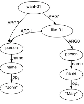
We first evaluate our algorithm on Abstract Meaning Representation (AMR) (Banarescu et al. 2013). AMR is a semantic formalism where the meaning of a sentence is encoded as a rooted, directed graph. Figure 8 shows an example of an AMR graph in which the nodes represent the AMR concepts and the edges represent the relations between the concepts they connect. AMR concepts consist of predicate senses, named entity annotations, and in some cases, simply lemmas of English words. AMR relations consist of core semantic roles drawn from the Propbank (Palmer, Gildea, and Kingsbury 2005) as well as very fine-grained semantic relations defined specifically for AMR. We use the training set of LDC2015E86 for SemEval 2016 task 8 on meaning representation parsing (May 2016), which contains 16,833 sentences. This data set covers various domains including newswire and Web discussion forums.
For each graph, we derive a vertex order corresponding to the English word order by using the automatically generated alignments provided with the data set, which
want-01
person
like-01
ARG0 ARG1
ARG1
name
“John”
name
op1
person
name
“Mary”
name
[image:22.486.51.187.469.637.2]op1 ARG0
Figure 8
0 1000 2000 3000 4000 5000 6000
[image:23.486.54.235.62.183.2]0 1 2 3 4 5 6 7 >=8
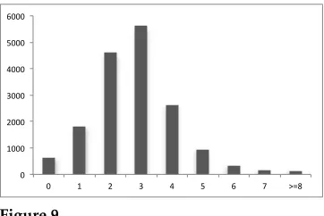
Figure 9
The distribution of AMR relative treewidth.
align tokens in the string to concepts or edges in the graph. We first collapse subgraphs of named entities and dates to a single node on the graph side. For example, the subgraph corresponding to “John” is collapsed to a single node “person+John,” and the same goes for the subgraph for person name “Mary.” There are also some vertices in the graph that are not aligned to any token. We want to linearize all vertices (concepts) in the graph in such a way that the string side order is kept as much as possible (we call it string order). We first sort the aligned vertices according to the position of their token side. We use the first position in case a vertex is aligned to multiple positions. If an unaligned vertex is the parent of an aligned vertex, we insert it right before the aligned vertex in the sequence. Otherwise, for simplicity, we append the unaligned vertex to the end of the vertex sequence, according to its relative order in the depth-first traversal of the graph.
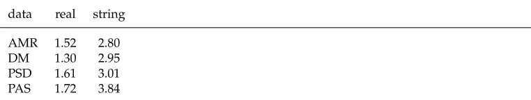
After we have constructed the input vertices with vertex order π, we run Algo-rithm 1 to determine the relative treewidth of each AMR graph with respect to the vertex orderπ. Figure 9 shows the distribution of relative treewidth of AMR graphs in the data set. We can see that over 99% of the AMR graphs can be built using a cache size of 8. As shown in Table 1, the average relative treewidth with respect to the string order is 2.80. The average treewidth of this data set (i.e., the average of minimum relative treewidth of each AMR graph with respect to any vertex order) is 1.52. This shows that using the string order as a constraint does not significantly increase the treewidth statistics of the data set.
Table 1
Relative treewidth statistics with respect to different vertex orders: “real” means the real treewidth of the data, “string” means using the string order constraint, “gold” means using the gold alignment.
data real string (gold) string reversed string reversed string random
(gold)
LDC2015E86 1.52 - 2.80 - 3.08 4.84
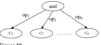
[image:23.486.52.435.600.663.2]Figure 10
The AMR subgraph representation for the substringc1,c2,. . .andcn.
In the worst case, the maximum relative treewidth of a graph can be 16, while the maximum treewidth of the data is 4. This is because when using the string order as a constraint for the vertex order, the string-to-vertex alignment does not always follow the preorder traversal of vertices that is desirable in the width computation. The most problematic case is the traversal of a node with many branches, with op’s structure most significant in the AMR data. For example, in Figure 10,n different concepts are connected to the parent concept “and” with the opk(k=1,· · ·,n) relation. This structure
does not introduce high treewidth because we can put “and” and eachciinto a separate
bag, forming a chain of bags of width 1. However, when we use the string order as a constraint, we first introduce verticesc1,c2,. . .,cn−1, then we further introduce “and” andcn. This would result in a chain structure of length (n+1) in the tree decomposition,
where “and” is introduced at the n-th bag in the chain. According to Algorithm 1, becausec1,c2,. . .,cn−1 are all introduced above the bag that introduces “and” and all connect to “and,” the relative treewidth is at leastn−1. In general, a high-branching structure with most children introduced before the parent would result in larger relative treewidth and distort from the real treewidth of the graph.
Another reason for high relative treewidth is the alignment errors from the auto-matic alignments. When multiple instances of the same word align to multiple vertices with the same concept labels, the automatic alignment usually cannot distinguish them and often creates a many-to-many alignment between instances of the word in the string and instances of the concept in the graph. This results in a wrong traversal order of the multiple vertices and a larger relative treewidth. Our worst-case sentence, with relative treewidth of 16, is due to this type of error in the automatically generated alignments.
We additionally experiment on a smaller data set of 200 hand-aligned AMR/English sentence pairs by Pourdamghani et al. (2014). From Table 1, we can see that the average relative treewidth of these AMR graphs with respect to the string order is 2.61 when using the gold alignment, and the average treewidth is 1.43. If we use the automatic alignment for these AMRs, the relative treewidth becomes 2.68. The maximum relative treewidth for both cases are 6. This number is much lower than the maximum relative treewidth of the LDC2015E86 training data because the maximum sentence length of the smaller data set is 54, whereas for the latter data set the maximum sentence length can be as large as 225. By comparison, we can also see that alignment errors can result in higher relative treewidth, though not significantly.
relative treewidth is 3.08. This number is slightly larger than using the string order. The reason might be that English is more likely to have relation arcs going from left to right. If we randomize the vertex order, the relative treewidth becomes 4.84.
We also evaluate the coverage of our algorithm on semantic graph-based represen-tations other than AMR. We consider the set of semantic graphs in the Broad-Coverage Semantic Dependency Parsing task of SemEval 2015 (Oepen et al. 2015), which uses three distinct graph representations for English semantic dependencies.
r
DELPH-IN MRS-Derived Bi-Lexical Dependencies (DM): Thesesemantic dependencies are derived from the annotation of Sections 00-21 of the WSJ Corpus with gold-standard HPSG analyses provided by the LinGO English Resource Grammar (Flickinger 2000; Flickinger, Zhang, and Kordoni 2012). Among other layers of linguistic analysis, this representation also includes logical-form meaning representations in the framework of Minimal Recursion Semantics (MRS) (Copestake et al. 2005).
r
Enju Predicate-Argument Structures (PAS): This data set comes from theHPSG-based annotation of Penn Treebank, which is used for training the wide-coverage HPSG parser Enju (Miyao 2006). Enju can effectively analyze syntactic/semantic structures of English sentences and output phrase structures and predicate-argument structures with a wide-coverage grammar and a probabilistic model trained on this data.
r
Prague Semantic Dependencies (PSD): The Prague Czech-EnglishDependency Treebank (Hajic et al. 2012) is a set of parallel dependency trees over the WSJ texts from the Penn Treebank, and their Czech translations. The PSD bi-lexical dependencies have been extracted from what is called thetectogrammaticalannotation layer (t-trees). We experiment on the English part of the treebank in this article.
[image:25.486.54.435.587.659.2]Differently from the case of AMR, in all of these graph representations the vertices are exactly the tokens from the input string. From Table 2 we can see that using English word order as the vertex order, the average relative treewidth for the set of DM graphs is 2.95, while the average real treewidth of the DM graphs is 1.30. The PSD and PAS graphs have larger real treewidth in comparison with the DM graphs, and the relative treewidth is also larger. We also observe that even though DM has smaller average
Table 2
Relative treewidth statistics for SemEval 2015 semantic dependency graphs.
data real string
AMR 1.52 2.80
DM 1.30 2.95
PSD 1.61 3.01
0 2000 4000 6000 8000 10000 12000 14000 16000 18000 20000
[image:26.486.49.259.61.204.2]0 1 2 3 4 5 6 7 >=8 DM PSD PAS
Figure 11
The distribution of relative treewidth for SemEval 2015 semantic dependency graphs.
real treewidth in comparison with AMR, the relative treewidth is slightly larger. This is because articles, prepositions, and other non-content words appear as vertices in DM graphs, whereas in AMR these words appear either as edges or not at all. Articles in particular increase the relative treewidth, because the article appears as a left neighbor of the head noun in the semantic dependency graphs, and the number of left neighbors of a vertex is a lower bound on relative treewidth, as discussed earlier in relation to conjunctions in AMR. We find that whereas most AMR graphs have relative treewidth of 2 or 3 (shown in Figure 9), most semantic graphs in the Semantic Dependency Parsing data sets have slightly larger relative treewidth (3 for DM and PSD, and 3 or 4 for PAS, shown in Figure 11). With a cache size of 8, the coverage rate is 100% for DM and over 99% for PSD and PAS. In practice, we can tune the cache size to optimize the trade-off between coverage and the ease of prediction.
To summarize, we find that the relative treewidth of the analyzed semantic graph-based structures, with respect to the English word order, is low enough to make efficient parsing possible. Furthermore, the fact that the real word order results in lower relative treewidth than random orders, or even the reverse order, indicates that the real English word order provides valuable information that our parsing framework can exploit.
7. Comparison with Other Formalisms
In this section we compare our cache transition parser with existing formalisms that have been used for graph-based parsing, as well as to similar transition-based systems for dependency tree parsing.
7.1 Connection to Hyperedge Replacement Grammars
S →
X
1 2
X
1 2
1
→
2
X
1 2
X
1 2 →
[image:27.486.56.323.64.281.2]1 2
Figure 12
An HRG that generates cycles of any size. Squares indicate grammar nonterminals with numbered ports. Number above vertices in a rule’s right-hand side correspond to the ports of the lefthand side nonterminal. An example derivation is shown in Figure 13.
HRGs contain rules that rewrite a nonterminal hyperedge into a graph fragment consisting of a number of new nonterminal hyperedges and terminal edges (see the example grammar in Figure 12). The vertices that a nonterminal hyperedge connects to, known as itsports, are also the points at which the rule’s right-hand side graph fragment is attached to the rest of the graph after the nonterminal is rewritten. An HRG derivation of a graph can be viewed as a derivation tree, with a grammar rule at each node, where the rule expanding a nonterminal hyperedge is a child of the rule that introduced the nonterminal in its righthand side. This derivation tree provides a tree decomposition of the derived graph. More precisely, the tree decomposition has the same nodes and the same branching structure as the derivation tree, and each bag in the tree decomposition contains all the vertices that appear in the right-hand side of the rule.
In the other direction, it is possible to extract HRG rules from a tree decomposition by treating each bag as a rule. Nonterminals in the extracted rules correspond to the arcs of the tree decomposition. For an arc (i,j) of the tree decomposition, letXiandXj
be the bags at nodesiandj, respectively. The set of verticesXi∩Xj, known as the arc’s
separator, are the vertices to which the corresponding HRG nonterminal was connected before being rewritten.
Example 5
S ⇒ v1 v2
X
1 2
⇒ v1 v3 v2
X
1 2
⇒ v1 v3 v4 v2
X
1 2
⇒ v1 v3 v4 v2
v1,v2
v1,v2,v3
v2,v3,v4
[image:28.486.51.355.69.278.2]v2,v4
Figure 13
An example derivation of the HRG from Figure 12 (left), along with the corresponding tree decomposition of the derived graph (right). Each bag of the tree decomposition corresponds to one rule application in the derivation.
Because each run of our parser corresponds to a smooth tree decomposition, it is possible to describe a corresponding HRG. This HRG will have a number of specific properties. Because our tree decompositions are smooth, the HRG rules will always introduce exactly one new vertex in their right-hand side. Because the separators of a smooth tree decomposition of treewidth k all contain kvertices, the nonterminals of the derived HRG all have exactly kports. The branching factor of a node in our tree decomposition corresponds to the number of right-hand side nonterminals in the corresponding HRG rule, and is potentially unlimited.
In general, the branching factor of the tree decompositions produced by our parser is not bounded by a constant, while any fixed HRG has a maximum number of right-hand side nonterminals in its rules. This implies that, although it is possible to extract an HRG corresponding to one run of our parser, it is not always possible to produce an HRG whose derivations correspond to all possible runs of a parser. We emphasize that these observations apply to the derivations of the HRG rather than to the language of graphs produced. It is an open question whether all the graphs of fixed relative treewidth with respect to a vertex order can be generated by a fixed HRG.
7.2 Connection to Existing Transition-Based Systems
We have already mentioned that when we use a cache with size 2, we can only construct graphs that are trees. This follows from the fact that any graph with at least one cycle has relative treewidth larger than one, and thus cannot be parsed with cache size 2, by Theorem 1. When the cache size is bounded by two, the edge construction operations that are available to the parser resemble the left-arc and the right-arc transi-tions of the arc-standard parser described by Nivre (2008), if we disregard the fact that these transitions remove the dependent vertex from the stack. However, this similarity is only superficial and the two parsers are incomparable, as explained subsequently.
The arc-standard parser can construct trees in which the root is at the rightmost position of the input string, and all of the remaining tokens are left children of the root. As already discussed in Section 6, such trees have relative treewidth proportional to the length of the string. By Theorem 1, these trees cannot be parsed with cache size of 2.
In the opposite direction, when using cache size of 2 we can construct non-projective trees, something that is not possible with an arc-standard parser. As a simple example, consider the non-projective dependency tree G shown in the left part of Figure 14, where we have disregarded the edge directions. The derivation tree in the right part of Figure 14 displays a run of a parser with cache size 2 constructingG. When vertices
v1andv2are in the cache for the first time, the parser constructs the edge (v1,v2). It then pushesv3into the cache, movingv2out of the cache and into the stack and constructing the edge (v1,v3). It then popsv3 from the cache, moving back to the configuration with cache contentv1,v2. Next, the parser pushesv4into the cache, movingv1into the stack and constructing the edge (v2,v4). Afterward, it popsv4 from the cache, again moving back to the cache contentv1,v2. Two more pops conclude the computation.
The fact that we can build non-projective trees, even with the minimum cache size of 2, is explained by the capability of our parser to use the cache to “reorder” vertices with respect to their original ordering in the input. In our example, for instance, at some step in the computation we havev2 in the stack andv1,v3 in the cache in the given order. This reordering of the input tokens is somehow reminiscent of the parsing model proposed by Nivre (2009), where a special transition called swap is used to reorder the input tokens and to construct non-projective dependency trees.
An alternative model for parsing non-projective dependency trees has been pro-posed by Attardi (2006). This parser constructs edges by connecting vertices in the stack that are not at adjacent positions, using special transitions called left-arckand right-arck
v1 v2 v3 v4
•
[$, $]
•
[$,v1]
•
[v1,v2]
•
[image:29.486.56.331.525.626.2][v1,v3] • [v2,v4]
Figure 14
Non-projective treeG(left), and derivation tree of a parser with cache size two constructingG