Dynamics of the small farmers’ behaviour – scenario simulations  

The number of small farms with diversified eco-nomic activities has been growing in the recent years. The rationale behind this growth is, however, not uniform. The reasons vary from pure economic and market considerations to clearly personal interests. The explanation of the farmers’ decision-making is further complicated by the lack of accurate data as farmers are not obliged to supply structured data, or some statistical evidence. Moreover, small farmers are often driven by different objectives than the profit maximisation; as the personal satisfaction and family tradition play the important role. Small farmers often employ family members, thus the organisation is typi-cally built on informal relationships. Despite these difficulties, we have mapped the farmers’ behaviour and designed the business model that advocates the diversification as a safety step to acquire and maintain the farmers’ secure position.

The Ministry of Agriculture of the Czech Republic pays more and more attention to the small farmers. The European Union approved the Rural Development Programme for period 2014–2020 with special

measures to support the small farmers (Ministry of Agriculture of the Czech Republic 2015a). According to the FAO (Vorley et al. 2008: 3) “The business model critically impacts on how value is created, captured or shared by farmers, SMEs and other chain actors. It is therefore important to establish inclusive, equitable and sustainable business models for farmers and SMEs. Factors which influence sustained and equitable inclu-sion of smaller scale farmers and SMEs are producer organization, market coordination and intermedia-tion, business support and financial services, buyer behaviour, and enabling policies and infrastructure”. The business model shows the basic principle how an organization creates, transmits and receives value. It is a useful strategic tool (Osterwalder et al. 2005). The aim of this paper is to simulate the scenarios of the possible development of individual farmers. At first, we build the business model that depicts the way of farmers’ behaviour and understanding of their market behaviour. Then, we transform that point of view into the computer simulation model using the system dynamics approach. We build the model

Dynamics of the small farmers’ behaviour – scenario

simulations

Gabriela KOLACKOVA*, Igor KREJCI, Ivana TICHA

Faculty of Economics and Management, Czech University of Life Sciences Prague, Prague, Czech Republic

*Corresponding author: kolackovag @pef.czu.cz

Kolackova G., Krejci I., Ticha I.: Dynamics of the small farmers’ behaviour – scenario simulations. Agric. Econ. – Czech, 63: 103–120.

Abstract:Th e paper deals with the dynamic simulation of the possible development scenarios of small farmers. Th e model is based on the offi cial data sources but also on the qualitative research of small farmers. Th e modelling structure refl ects the specifi cs of the examined fi eld and personal and social specifi cs of small farmers. For the purposes of the analysis, the business model describes the value creation in the small and individual farms, thereafter the model is extended into the dynamic simulation model and the selected scenarios of development are simulated. Th e analysis shows the impact of the current setup in the fi eld. Despite the fact that the paper contains the optimistic scenarios, a simple change of parameters leads to an unsustainable situation. Th e pessimistic scenarios grow from the realistic conditions when the parameters re-fl ect the recent period settings. Th is clearly depicts the infl uence of the weak market position of the farmers and advocates the diversifi cation tendencies.

Keywords:farmer, system dynamics, computer simulation, business models, scenarios

on the basis of the official data and the information from the qualitative research and simulate multiple scenarios afterwards. On the basis of the simulated scenarios, we build the new business model, which ultimately leads to an increase of the farmers’ inde-pendence and stability.

The article is structured as follows: the first part of the paper focuses the brief theoretical background of business models and the application of system dynamics on agricultural problems. In the second part, we describe the data sources, data consolidation and implemented model, respecting the qualitative information collected from the interviews. The main part of the article deals with the results, where the selected scenarios of farm development are presented in a greater detail. Discussion and possible applica-tions of the achieved results conclude the article.

BUSINESS MODELS

Beierlein et al. (2014: 1) claim, that “today’s agri-food system is a global, fast-paced, high-technology industry that is one of the most effective adopters of scientific innovation. Managers in this industry must be well grounded in the technical aspects of food and fibre production as well as the principles of business management.” In accordance with this, Žídková et al. (2011) mention in their research that especially on the level of agriculture, there is a num-ber of changes in the economic policy of the state on the national economy level. They state that the “farming enterprises were adapting to the changes in the business environment during the whole studied period” (Žídková et al. 2011: 41). The agricultural sector is specific by its seasonality of production, a high dependence on natural conditions, but also its production structure. These specifics are reflected in the profit or loss of the farms and also have an impact on the setting of their capital structure (Hlavsa and Aulová 2013). A correctly adjusted business model and business plans help to increase the competitive-ness of farms, which is in line with the conclusions of Dzodzi and Awetori (2013).

The business model is connected with the business strategy, which is the process of designing the busi-ness model and busibusi-ness operations (implementation of the company’s business model into organizational structures and systems) (Vorley et al. 2008). George and Bock (2011) discovered that the basic dimensions of the business model are structure of resources and

value structure. These results provide new directions for the development of the theory and empirical studies in business by linking the business model, co-creation opportunities and organizational out-comes. Therefore, the business model is a strategic analytical tool which defines how the company cre-ates and captures value (Chesbrough 2002; Pigneur and Tucci 2005; Zott and Amit 2008; Osterwalder and Richardson 2008). Value relates to the product (goods and/or services), process, assets and activi-ties associated with costs. Afuah and Tucci (2000) mention the business model as a method where the company uses its available resources better than the competition. It is a system of components that are con-nected by channels and their dynamics. Osterwalder (2013) compares a business model to a description how the company creates value. Teece (2010) adds that business models are a valuable tool also in the extrapolation of innovation and profit, understand-ing that the business model helps to understand the nature of organization, and the status of entrepreneurs and managers in the company.

SYSTEM DYNAMICS

As far as the term “business model” could be used also in the general way as any model of some busi-ness, the system dynamics models are well specified. Understanding the structure of the system brings the knowledge about the sources of the system’s behaviour. However, the complex dynamic systems are character-ised by the complex structure of feedbacks, the delays between action and reaction and the non-linear be-haviour (Meadows 2008; Sterman 2000). Considering the limited possibilities of human brain and building on the basis of the bounded rationality (Simon 1956, 1979) and mental models with the limited number of possibly reflected variables (Miller 1956; Doyle and Ford 1998; Cowan 2001), systems dynamists stress the necessity of the computer simulation as an important tool to support of the understanding of the system (Forrester 1961; Sterman 2000; Mildeová et al. 2012). Osterwalder et al. (2005) clearly connect business models (as defined above) and system dynamics when stressing that the testing and simulation of business models leads to lowering of risks and preparation for the future without endangering the business.

information and the model must be robust under all conditions (Coyle 1996; Sterman 2000). As the above described business models explain the value creation, the system dynamics model interprets the behaviour of the modelled system. Since the aim is the understanding of dynamic complex systems, the results of system dynamics models primarily stress the accuracy of behaviour before the numerical precision (Forrester 1987a; Sterman 2000).

Weber and Schwaninger (2002) apply system dy-namics to analyse the organisation and distribution system of cooperatives in the Swiss agribusiness (mainly SMEs), which triggered the reorganisation project and significantly changed the participants’ mental models. Shi and Gill (2005) searched for the policies of sustainable ecological agriculture in the county in China using the system dynamics model. The model identified the crucial factors for the promotion of sustainable ecological agriculture. Rozman et al. (2012a, b) introduce the system dy-namics model, which shows that the subsidies are the main source of the conversion from conventional to organic farming in Slovenia, however, the subsidies cannot be provided on the level that would complete the conversion. Li et al (2012) simulate the long-term trends of organic agriculture in the province in China, showing the current disadvantages and limits (such as a high methane production and an unsustainable energy structure) that could restrict the future development.

MATERIAL AND METHODS

For the quantification of the model parameters, we mainly use the agriculture and National Accounts Statistics from the Czech Statistical Office (2015a, 2015b) and the statistics on costs of agricultural products from the Institute of Agricultural Economics and Information (2014). The source of parameters is specified in the text. The aims of the farmer and thus the model structure is based also on the qualitative research among the Czech small farmers.

For the purposes of the research, we had to clarify the connection between the statistical classifica-tion and the meaning an average farmer. The Czech Statistical Office (2015a) understands the farmer as the Agricultural entrepreneur – natural person. According to the main production of this category, the

average farmer belongs to the group 01.11 (Growing of cereals (except rice), leguminous crops and oil seeds) and partly 01.4 (Animal production) from the CZ-NACE (Classification of Economic Activities) and the CZ-CPA (Classification of Products) point of view and belongs to the institutional sub-sector 142 (Recipients of Property Income and Transfers) from the Classification of Institutional Units (Czech Statistical Office 2015c).

To reveal the goals and to understand the basic be-haviour of farmers, we performed in-depth interviews during Spring 2014 among 24 farmers who met the above classification of the average small farmer1_{. The} size of the sample for that kind of qualitative research was chosen according to Warren (2002), where the new farmers were interviewed until the answers became repetitive, Karlíček (2013). The result of the in-depth interviews is that the majority of farms is focused only on agriculture, especially the plant production, which does not need such an intensive daily care as the livestock production. Farmers consider the pos-sibility of diversification as the option to devote to other activities of their interest but they understand the diversification as the way to spreading the risk and lowering their dependence on the suppliers and customers. However, they rarely take the decision to diversify.

Among others, the interviews concluded into few points that must be reflected by the following models: – Seasonal dependency

– Dependency on subsidies and the related support from the European Union and the government of the Czech Republic

– Family members often replacing the paid staff – Almost no investment on advertising

– The prevailing plant production over the livestock production

– Farmers have in average 5 heads of livestock (not for business, but for the full farm characteristic and the farmer’s hobby)

– Owner’s satisfaction is superordinate to profitability The basic business model was compiled on the basis of the qualitative study, see Figure 1. The design of template was made from the components of the Canvas Business Model (Osterwalder and Pigneur 2010) in the combination with the Holloway and Sebastiao (2010) and Shafer et al. (2005) technique. Poláková et al. (2015) describe how this combination was developed in their research.

Th e result is a new model which refl ects the value creation. Th e value proposition is generated from the interaction between the owner, farm environment and customer. The following three items have an effect on the model – key partners (who have the infl uence on the production or activity of the farm), customer relationship, communication channel (how the prod-uct is off ered to the customer). Cash fl ow follows the decisions and behaviour of the right side of the model.

To test the possibilities and to identify the risks of being an average small farmer, we created the simulation model, which respects both the official

data and findings from the interviews. To specify the behaviour of the small farmer, we transformed the Business model from 1 into the causal loop diagram.

Figure 2 shows the high level causal loop diagram, which is summarising the main feedbacks in the small farm’s dynamic model. The positive link polar-ity denotes that if everything else remains and the initial (independent in the link) variable increases/ decreases, then the target (dependent in the link) variable increases/decreases above/below the level where it would have been (e.g. if Land increases, then Land cost increases too). On the other hand, the negative polarity denote that if the initial variable increases/decreases, then target variable decreases/ increases below/above the level where it would have been (e.g. the lower is the Fixed capital stock, the higher must be Investments)2.

For the modelling starting point, we assumed that the farmer has the possibility to decide when to buy or acquire new land (according to the profit, see the balancing loop B1). We also simulate the scenarios that the farmer buys the new land when such opportunity occurs, without the connection to the actual profit, the size of the farm or savings. Balancing loop B2 shows the feedback that the in-creasing profit leads to the increase of the land and the consequent necessary investments into capital, which balances the profit. B3 only balances the neces-sary investments according to fixed capital stock, the more capital the farmer owns, the less investments

Figure 1. Specific Business Model for the small and individual farms

Figure 2. Overview of the model feedback structure

2_{For more about causal loop diagrams, see e.g. Sterman (2000) or Coyle (1996)}

1. Owner

– Personality – owner’s satisfaction is superordinate to profi tability – Knowledge – Interests – Hobbies Renevue stream:

subsidies, selling agriculture products

Cost structure: Land cost, land aquisition, investment, operation and

reconstruction, animal acquisition, other fi xed

and variable costs

3. Customer

– Purchaser agricultural production

Relationship

4. Value proposition

plant production

Key Partners – Ministry of Agriculture and other government institution, main

suppliers, local authority, association

for breeder

2. Farm’s environment

– Nature (character) – Location – weather – Buildings and equipment – Livestock

– Land – quality and quantity – People – family, staff

into new capital are necessary. Balancing loop B4 is similar to B2, but the profit is balanced through the necessary expenditures into the renewal of the exiting capital. As the qualitative research showed, the farmers’ satisfaction with the farm management is based also on the ownership and care for animals. Nevertheless, the model of the farm contains animals as an inseparable but only a hobby part of the farm system without market production. Balancing loop B5 shows that with the increasing number of animals, the satisfaction grows and as a result, the scope of the new acquisitions of the animals is decreasing.

The production part of the model contains two self-reinforcing feedbacks R1 and R2, which would lead to the exponential growth of the farm if not limited by the balancing loops and exogenous limits. Small farmers’ profit is increasing because of the sold yield and subsidies. Both feedbacks are based on the size of the farm.

The land represents the crucial stock variable for the farmer. Figure 3 shows the stock and flow dia-gram of the land subsystem. The land stock (stocks are represented by the box variable) increases by the inflows representing renting and buying of the new land and decreases by the outflow termination of the rental of the land (flow variables are represented by pipes with faucets). For the model purposes, we assume that the farmer does not sell any land.

Equations (1) – (3) describe the computation of the land stock in the simulation model, where T₀

is the initial time, T is the current time and t is any moment between T₀ and T. The average net rentals are the exogenous variable3.

න ሺܮܽ݊݀݌ݑݎ݄ܿܽݏ݁ݏ௧ሻ ்

்బ

݀ݐ ൅ ܱݓ்݈݊ܽ݊݀బ (1)

ܴ݁݊ݐ்݈݁݀ܽ݊݀ ൌ න

න ሺܮܽ݊݀݌ݑݎ݄ܿܽݏ݁ݏ௧െ ܴ݁݊ݐ݈݈ܽܿܽ݊ܿ݁ܽݐ݅݋݊௧ሻ ்

்బ

݀ݐ ൅

൅ ܴ݁݊ݐ்݈݁݀ܽ݊݀బ (2)

ܮܽ݊݀ݐ݋ݐ݈ܽ ൌ ܱݓ݈݊ܽ݊݀ ൅ ܴ݁݊ݐ݈݁݀ܽ݊݀ (3) For the purposes of the initial stock value and the model behaviour testing, it is necessary to choose the proper statistic of the average land. Due to the fact that agriculture is surveyed by multiple institutions, the data are very often incompatible and the same indicator is represented by highly various numbers. Different thresholds for Green Report (Ministry of Agriculture of the Czech Republic 2015b) and the Farm Structure Surveys (Czech Statistical Office 2015a)4 lead to a significantly different amount of our aim group of agricultural entrepreneurs – natural persons. While the Ministry presents 26 076 subjects, the Czech Statistical Office publishes only 16 523 per-sons in year 2013. The resulting average utilised ar-able land in 2013 would be 23.2 ha according to the Green Report, but 36.8 ha according to the Structure

Figure 3. Stock and flow diagram of the farmers’ land subsystem

3_{The development of exogenous variables is in the Annex I.}

4_{For example, the minimum 1 ha of utilised agricultural area in Green Report vs. 5 ha in the Farm Structure Survey or}

Survey. Our model depicts the farmer that focuses on the cereals production as his/her main income. This is why we prefer higher threshold from the Czech Statistical Office. Since the difference equals to more than 9.5 thousand of farmers, it represents the farmers that satisfy the Green Report threshold, but do not reach the Structure Survey threshold (e.g. more than 1 ha but less than 5 ha), the group consists of persons with the marginal scope of agricultural production. It is hardly acceptable that farming is the main occupa-tion for these persons. For the purposes of the paper, we generalise the difference between the surveys as the group of mainly occasional and hobby farmers that do not correspond to the definition of the small farmer used in presented research.

Moreover, the thresholds are in the logical disjunc-tion (OR), therefore, we reclaimed the data from the Structure Survey only on farmers that really utilise the land (i.e. without pure animal producers which do not utilise any land). As a result, the average utilised arable land in 2013 of agricultural entrepreneurs – natural persons that utilise land according to Structure Survey is 50.7 ha.

The total revenue comes from the total land, the average yield per ha and price per ton. The revenue from yield is calculated from (4)–(6). The index p represents the type of production. The model con-tains the three dominant crops – winter wheat, spring barley and rape. The Shares of the crops in the total land, Yield per ha and Price per ton of production are exogenous variables, Price per ton of production is included in three variants as bread and feed qual-ity and average of these prices. Average subsidiesto land represents the exogenous variable based on the data from Foltýn et al. (2010) and the Institute of Agricultural Economics and Information. The vari-able also includes the average investment subsidies per ha calculated on the basis of data from the Czech Statistical Office (2015a).

Total yield = Total land_p × Yield per ha_p (4)

Revenue from yield_p =

Total yield_p × Price per ton of production_p (5)

Revenue from yield = Σ_p Revenue from yield_p (6)

The land as production factor is not connected only with the outputs, but we have to reflect also the

necessary inputs. Average land utilisation costs are different for each kind of crop (fertilisation, seeds, crop protection etc.). Data are from the Institute of Agricultural Economics and Information (2014). Because the simulation model contains the separate fixed capital and labour subsystem, these costs are applied without depreciation and labour costs.

Land utilisation expenditures_p =

Total land_p × Average land utilisation costs_p (7) Land utilisation expenditures =

Σ_p Land utilisation expenditures_p (8)

Variable Land price and Average land rent are ex-ogenous variables. Data are from the Ministry of Agriculture of the Czech Republic (2012). The data source contains the price of the land from different sources, which can significantly differ. For the model purposes, we use the Czech Statistical Office data, which are based on the tax return evidence, other sources published by the Ministry of Agriculture of the Czech Republic (2012) do not include the sample of such size and are usually focused on clearly market prices. For the model purposes, we need the price for which the land was really sold and purchased, which also includes the prices lowered informal effects (e.g. family bonds). Such prices are reflected by the Czech Statistical Office data source.

Rental expenditure = Average land rent × Rent land (9)

Purchase expenditure =

land price × Land Purchases (10)

Similarly to the land production, the model con-tains the animals. Figure 4 shows the stock and flow diagram of the animal subsystem. For the purposes of the model, we abstract from calf breeding, there-fore, the livestock increases only by the inflow of the livestock acquisition and decreases by deaths.

Equations (11)–(15) depicts the basic dynamics of the livestock. Average length of life is constant equal to 20 years5_{, Average subsidies to livestock, Average price} of livestock unit and Average animal care costs are exogenous variables from the Czech Statistical Offi ce (2015a), the Institute of Agricultural Economics and Information, Foltýn et al (2010). Due to the fact that the price depends on the weight, we assume 700 kg cattle, the subsidies are set according to suckler cows. Similarly to crop production in the land subsystem, the

5_{The life expectancy respects the hobby purpose of the breeding, even the half Average length of life was tested}

Animal care expenditures do not contain labour costs and depreciation, the variable contains direct material such as the consumption of feed or medication and the outsourced services as the veterinary care etc. (Institute of Agricultural Economics and Information 2014).

ܮ݅ݒ݁ݏݐ݋்ܿ݇ൌ

න ሺܮ݅ݒ݁ݏݐ݋ܿ݇ܽܿݍݑ݅ݏ݅ݐ݅݋݊ݏ௧െ ܦ݁ܽݐ݄ݏ௧ሻ ்

்బ

݀ݐ (11)

Deathsൌ ௅௜௩௘௦௧௢௖௞

஺௩௘௥௔௚௘௟௘௡௚௧௛௢௙௟௜௙௘ (12)

Subsidies to livestock = Livestock × Average

subsidies to livestock (13)

Acquisition expenditures = Livestock acquisition × Average price of livestock unit (14)

Animal care expenditures = Livestock × Average animal care costs (15)

The livestock acquisition impulse comes from the Desired size of livestock, which is equal to 5 on the basis of qualitative research. For the purpose of pa-rameters estimation and some scenarios, we assume that the farmer decides to purchase animals from the specific size of the farm, which is expressed by the variable Required size of the farm. Variables Time to correct livestock and Required size of the farm are parameters that will be estimated later.

Desired size of livestock = 5, for

Land total ≥ Required size of the farm (16)

Desired size of livestock = 0, for

Land total < Required size of the farm 17)

Desired livestock correction =

Desired size of livestock – Livestock (18)

Livestock acquisition ൌ஽௘௦௜௥௘ௗ௟௜௩௘௦௧௢௖௞௖௢௥௥௘௖௧௜௢_{்௜௠௘௧௢௖௢௥௥௘௖௧௟௜௩௘௦௧௢௖௞} (19)

Although it is possible to use bookkeeping data on capital in some sort of analysis (Čechura 2012; Pechrová 2015), it is recommended to use the outputs of the Perpetual Inventory Method (PIM) for the economic analysis of fixed capital. Since business bookkeeping contains the data on fixed capital in historical prices (the stock value sums the prices from different years without revaluation) and de-preciation is not frequently based on the real service life of the asset, thus the still serving assets can have zero net book value, the book keeping is not usually suitable for the economic analysis (Pigou 1935; Hulten and Wykoff 1996; Diewert 2005; OECD 2009). Therefore, we adopt the parameters from the Perpetual Inventory Method (Czech Statistical Office 2002; OECD 2009).

Figure 5 shows the stock and flow structure of fixed capital. The Average service live is 25.05 years. This value is the 2004–2013 weighted average of service lives of all types of assets in the PIM (Czech Statistical Office 2002), where the weights are the values of net fixed capital stock in the CZ-NACE A (Czech Statistical Office 2015b).

The Average capital per ha and Average capital per livestock unit are calculated from the net capital stock in institutional sector 14 (households) in the CZ-NACE A (Czech Statistical Office 2015b). The capital is divided by the weighted total area of land in this sector and the weighted amount of livestock units in the sector. For weights, we used capital depreciation from the Institute of Agricultural Economics and Information (2014). The 2004–2013 average is 50 992.3 CZK for the Average capital per livestock unit and 27 036.2 CZK for the Average capital per ha.

‹š‡†…ƒ’‹–ƒŽ•–‘…ǡൌ න ൫˜‡•–‡––ǡȂ‘•—’–‹‘‘ˆˆ‹š‡†…ƒ’‹–ƒŽ–ǡ൯ ்

்_బ

†– ൅ ‹š‡†…ƒ’‹–ƒŽ•–‘…Ͳǡ (20)

ܥ݋݊ݏݑ݉݌ݐ݅݋݊݋݂݂݅ݔ݁݀ܿܽ݌݅ݐ݈ܽ_௠ൌ ܨ݅ݔ݁݀ܿܽ݌݅ݐ݈ܽݏݐ݋ܿ݇௠

ܣݒ݁ݎܽ݃݁ݏ݁ݎݒ݈݂݅ܿ݁݅݁ (21)

Desired fi xed capital_a = Livestock × Average capital per livestock unit (22)

Desired fi xed capital_b = Land total × Average capital per ha (23)

Desired capital stock adjustment_m = Desired fi xed capital_m – Fixedcapital stock_m (24)

Investment_m = MIN ܦ݁ݏ݅ݎ݁݀ܿܽ݌݅ݐ݈ܽݏݐ݋݆ܿ݇ܽ݀ݑݏݐ݉݁݊ݐ௠ ܶ݅݉݁ݐ݋݆ܽ݀ݑݏݐܿܽ݌݅ݐ݈ܽ௠ ൰

+ Consumption of fi xed capital_m, Maximum investment (25)

ܯܽݔ݅݉ݑ݉݅݊ݒ݁ݏݐ݉݁݊ݐ_௠ൌ ܯ݋݊݁ݕݏݐ݋ܿ݇

ܯ݅݊݅݉ݑ݉݅݊ݒ݁ݏݐ݉݁݊ݐݐ݅݉݁௠

(26) Equations (20)–(26) describe the basic dynamics of

the farmers’ fixed capital stock. The connection with other subsystems is via Livestock and Land total. The subscript m denotes the connection with livestock a or land b.

The farmer’s Investment is a simple function com-posed from new investments and replacement invest-ments (Jorgenson 1963, 1996). The function assumes the disequilibrium between the desired and actual capital, where the new investment does not fill the gap immediately but the process of investment is de-layed (Sterman 2000; Forrester 1987b). Time to adjust capital delay contains several factors: the investment

cautiousness, the decision making demandingness, but also the delays caused by the administrative per-missions and the construction time period in case of buildings etc. This parameter will be estimated later. The Equations (25) and (26) contain the decision between the “normal” investment described in the previous two paragraphs and the Maximum invest-ment. Such structure prevents the Money stock from being negative (Sterman 2000: 545–547). In this case, the investment falls behind the desired value and the gap is increasing, the investment will grow to the re-quired intensity when the Money stock is high enough. Minimum investment time will be estimated later.

Figure 6 shows the stock and flow structure of the money subsystem. In this subsystem, all expenditures and earnings that were introduced in the previous parts are integrated. This part also reflects the im-portant informal part of the small farmers’ existence, which is depicted in the lower part of the diagram. The farmers’ behaviour is strongly influenced by the family tradition and they overcome the bad pe-riods with the support of other family members and restrain themselves with the vision of better periods in future. For this purpose, we introduce the Self-debt stock variable, which integrates the difference between the average wages in the agriculture and the possible Labour expenditures in the average farm, i.e. what the farmer owe to himself/herself and his family. Once the profit is high enough, the self-debt is paid off.

Average gross wage is the exogenous variable based on data on the average gross monthly wage (Czech Statistical Office 2015d). Labour force is the func-tion of Land total estimated on the basis of the data from the Structure Survey (Czech Statistical Office 2015a). The data on labour force in the annual work

Figure 5. Stock and flow diagram of the farmers’ fixed capital stock subsystem

units (AWU) on the level of the Agricultural entre-preneur – natural person are not officially published and were prepared for the purposes of the paper6_. The delay parameter Time to pay off the self-debt will be estimated later.

Equations (27)–(35) describe the dynamics of the monetary part of the system.

The difference between the Desired self-debt pay off and the real Self-debt pay off (equal to Pay off

expenditures) is that the Self-debt payoff is non-zero only in the case that the current Labour expenditures deficit is equal to zero.

Similarly to (25) and (26), the equations (34) and (35) secure the non-negativity of the money stock, which is in correspondence with the idea of the self-debt derived from the qualitative part of the research. When the farmer finds the actual money stock insufficient, he/she lowers the labour

expen-‘‡›•–‘… ൌ න ሺ…‘‡–Ȃ’‡”ƒ–‹‘•‡š’‡†‹–—”‡•–Ȃƒ›‘ˆˆ‡š’‡†‹–—”‡•–Ȃƒ„‘—”‡š’‡†‹–—”‡•–ሻ

்

்బ

݀ݐ (27)

Income = Subsidies to livestock + Total subsidies to land + Revenue from yield (28)

Operation expenditures = Livestock acquisition expenditures + Animal care expenditures +

Land utilisation expenditures + Purchase expenditures + Investment_m (29)

Desired labourexpenditures = Average gross wage × Labour force (30)

Labour force = f(Land total) (31)

‡ŽˆǦ†‡„–ൌ න ሺƒ„‘—”‡š’‡†‹–—”‡•†‡ˆ‹…‹––Ȃ‡ŽˆǦ†‡„–’ƒ›‘ˆˆ–ሻ

்

்బ

݀ݐ ₍₃₂₎

‡•‹”‡†•‡ŽˆȂ†‡„–’ƒ›‘ˆˆൌ (33)

Labourexpenditures = MIN(Desired Labour expenditures, Maximum labour expenditures) (34)

ܯܽݔ݅݉ݑ݈ܾ݉ܽ݋ݑݎ݁ݔ݌݁݊݀݅ݐݑݎ݁ݏ ൌ ܯ݋݊݁ݕݏݐ݋ܿ݇

ܯ݅݊݅݉ݑ݈ܾ݉ܽ݋ݑݎ݁ݔ݌݁݊݀݅ݐݑݎ݁ݏݐ݅݉݁ (35)

6_{Statistics on the function (second order polynomial) of labour force are in Annex II.}

Figure 6. Stock and flow diagram of the farmers’ fixed capital stock subsystem

‡ŽˆȂ†‡„–

ditures to a smaller level that is appropriate to the actual money stock.

Figure 7 shows the simple land purchasing decision making. This structure is used only in the selected scenarios because we understand the possibility of continuous land purchases dependent on the farmers’ decision as too strong assumption. Commonly, the farmer does not have the possibility to choose and he/she buys the land when it is possible.

Equations (36)–(42) describes the decision mak-ing process. SMOOTHn function in (39) stands for nth order exponential smoothing, which is applied to the model as the perception of the actual variable (Sterman 2000: 428–436; Coyle 1996: 102–105). We use this formula to express the farmers’ adaptive ex-pectations. The farmer does not instantly/discreetly react on the changes of the crop and land prices, but has his/her own idea about the situation and this idea is continuously changing.

The farmer compares the Perceived net income from land with the price of the land. Once the ratio exceeds the threshold, he/she buys the land accord-ing to the difference between the threshold and the actual ratio. Variables Land price ration threshold, Purchasing effect of landexpedience, n and Time to perceive net income are to be estimated.

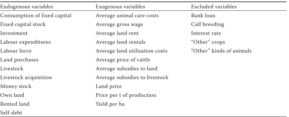
To summarise the previous description, the Table 1 expresses the model boundary. This table contains

the most important endogenous, exogenous and ex-cluded variables and thus depicts the simplification of the real system. Moreover, the exogenous variables describe the situation of the small farmers as pure receivers of the important decision variables without the chance to change their value (e.g. price of the ton of production). All parameters and exogenous variables are in prices of 2010.

Statistical estimations we conducted using the statistical software R version 3.2.1, for simulations we use the Vensimsimulation software. Simulation used the Euler integration with the time step set to dt = 0.03125. To search the values of the esti-mated parameters, we use the Powell optimisation (Dangerfield and Roberts 1999; Press et al. 1992) with the goal to minimise the difference from the official statistics on own land of the Agricultural entrepreneur – natural person (according to the current methodology available for 2000, 2010 and 2013), to minimise the difference between the Desired labour expenditures and Labour expenditures and to achieve the goal to have the desired livestock in 2012 at the latest. The whole model consists of 144 variables and parameters. The estimated parameters are as follows:

– Time to correct livestock – Required size of the farm – Time to adjust capital Figure 7. Farmers’ land purchasing decision making

ܰ݁ݐ݅݊ܿ݋݉݁݌݁ݎ݄ܽ ൌ (36)

Income from land = Revenue from yield + Total subsidies to land (37)

Land expenditures = Land utilisation expenditures + Consumption of fixed capital_b (38)

Perceived net income = SMOOTHn (Net income per ha,Time to perceive net income) (39)

ܮܽ݊݀݅݊ܿ݋݉݁ݐ݋݌ݎ݅ܿ݁ݎܽݐ݅݋ ൌ (40)

Land income expedience = Land income to price ratio – Land price ratio threshold (41)

Land purchases = MAX (Land income expedience × Purchasing effect of landexpedience) (42)

ܫ݊ܿ݋݂݉݁ݎ݋݈݉ܽ݊݀ െ ܮܽ݊݀݁ݔ݌݁݊݀݅ݐݑݎ݁ݏ

ܮܽ݊݀ݐ݋ݐ݈ܽ

ܲ݁ݎܿ݁݅ݒ݁݀݊݁ݐ݅݊ܿ݋݉݁

– Minimum investment time

– Minimum labour expenditures time – Time to pay off the self-debt

– n//order of exponential smoothing from equation (39) – Land price ratio threshold

– Purchasing effect of landexpedience – Time to perceive net income

Results of the estimation with multiple starts are in the Annex III.

Based on those data, we determined following sce-narios for research:

– Basic scenario (the average conditions and continual purchase of new land).

– Scenario of different variants of the production quality.

– The behaviour of farms in various ways to pur-chase new land (the average/5-years purpur-chases in 2001–2005/2004–2008/2007–2011)

– Optimistic/pessimistic/partly pessimistic I. and II. scenarios (the pessimistic scenario was based on the combination of the prices of production, yield, quality of production and possibility of purchase new land).

RESULTS AND DISCUSSION

Figures 8–10 show the basic model variables, which describe the situation of the farmer. This run is for the average quality of the yield, the acquisition of animals and the continuous land purchases without

Table 1. Small farmer model boundary

Endogenous variables Exogenous variables Excluded variables

Consumption of fixed capital Average animal care costs Bank loan Fixed capital stock Average gross wage Calf breeding

Investment Average land rent Interest rate

Labour expenditures Average land rentals “Other” crops

Labour force Average land utilisation costs “Other” kinds of animals

Land purchases Average price of cattle

Livestock Average subsidies to land Livestock acquisition Average subsidies to livestock

Money stock Land price

Own land Price per t of production

Rented land Yield per ha

Self-debt

0 1 000 000 2 000 000 3 000 000

2000 2001 2002 2003 2004 2005 2006 2007 2008 2009 2010 2011 2012 2013 2014 2015 2016 2017 2018 2019 2020

CZK

Desired fixed capital(b) Desired fixed capital(a) Fixed capital(b) Fixed capital(a)

Income Operations expenditures

0 100 000 200 000 300 000 400 000 500 000 600 000

2000 2001 2002 2003 2004 2005 2006 2007 2008 2009 2010 2011 2012 2013 2014 2015 2016 2017 2018 2019 2020

Year Slef-debt

Labour expenditures Desired labour expenditures

CZK

Figure 8. Farmers’ capital, income and operations

any maximum limit. The yield prices are set on the level of 2014 for the period 2015–2020, the land price set to 7-years moving average and rent are linearly extrapolated.

Each time the price of the yield drops, the farmer must save the money for the necessary expenditures and the self-debt grows. Self-debt starts to fall at the beginning of 2011.

Figure 11 compares the self-debt for a different yield quality. This is one of the most important parameters of the farmers’ performance. However, even the high quality yield could be sold only for the feed quality price. The low negotiation power of the farmer could lead to a lower evaluation of his/her production by the customer and due to his/her regional monopoly, the farmer could be forced to sell under the real value.

Scenarios with the mark II show the situation when the farmer cannot grow above the land area in 2010. The self-debt starts to decrease earlier due to the lower expenditures. Only one scenario has the mark III. In this case, the land area does not exceed the level in 2014. The area stabilisation in 2014 has an impact on the self-debt only in the feed quality sce-nario – the self-debt is stabilised and does not fall under 300 thousands CZK. In case of the average and bread quality, the income exceeds the expenditures, the money stock grows and, therefore, the self-debt is decreasing.

In all simulated scenarios, the increase of the land improved the money stock and the self-debt. However, the expenditures on land purchases rep-resent a significant part of the total expenditures. The Figure 12 shows the surplus of the money stock (Income – Operations expenditures – Desired labour expenditures) if the land prices linearly grows and the price per 1 ton of yield remains on the level of 2014. Each time the land area is stabilised and the Purchase expenditures become zero, the difference increases. Nevertheless, the highest slope of the line without stabilisation supports the requirement of the area growth.

Figure 13 compares five scenarios of land purchases on the self-debt indicator. All scenarios lead to the same land area 50.69 ha at the end of the 2013 (Czech Statistical Office 2015a). The basic run still applies the decision criterion from Figure 7. Scenario “Average purchases” shows the behaviour when each year the amount of the purchased land is same. Other three scenarios represent 5-year purchases, which do not

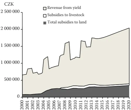
0 500 000 1 000 000 1 500 000 2 000 000 2 500 000

2000 2001 2002 2003 2004 2005 2006 2007 2008 2009 2010 2011 2012 2013 2014 2015 2016 2017 2018 2019 2020

CZK

Revenue from yield

Subsidies to livestock

Total subsidies to land

0 200 000 400 000 600 000 800 000 1 000 000

2000 2001 2002 2003 2004 2005 2006 2007 2008 2009 2010 2011 2012 2013 2014 2015 2016 2017 2018 2019 2020

CZK

Basic run Basic run II

Bread quality Bread quality II Feed quality Feed quality II Feed quality III

Figure 12. Difference between income and expenditures

Figure 10. Income composition – basic run _{Figure 11. Self-debt – yield quality impact}

–400 000 –300 000 –200 000 –100 000 0 100 000 200 000 300 000 400 000

2000 2001 2002 2003 2004 2005 2006 2007 2008 2009 2010 2011 2012 2013 2014 2015 2016 2017 2018 2019 2020 CZK

Basic run Basic run II

deserve the bank loan for the necessary expenditures (land utilisation, seeds etc.).

The delayed land purchases (2007–2011) show the best behaviour as the Labour expenses covered the Desired labour expenses in the best way and thus the self-debt stays very low in most of the examined period. Nevertheless, such scenario could be impos-sible to reach as the self-debt is low also because the smaller required Labour force. Small farm is usually held by the family members and thus it could be of-ten necessary to cover the higher labour force (more family members dependent on the family farm). The basic run with the decision criterion reaches the lowest maximum value. In all cases, the year 2011 is the turning point again. From 2011, the self-debt is decreasing and the money stock is growing.

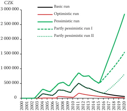
Figure 14 compares the pessimistic and optimistic scenarios. The self-debt is used as an indicator again as it is integrated in the lack of income in compari-son with the wages in the agriculture as industry (CZ-NACE A). In these scenarios, the data for the future Land price, Yieldper ha and Price per ton of production are on the 4-year minimum or maximum depending whether it is optimistic or pessimistic. Moreover, the optimistic scenario production is of the bread quality, the feed quality is applied in the pessimistic scenario. From the beginning of the 2015, the farmer in pessimistic scenario cannot purchase new land, buy new capital and does not have any wage for his/her effort.

Despite the fact that the scenario is called pessimistic, it is based on the prices of the selected crop from the year 2010 (2009 would be still worse) and the average yield from 2012 (rape, wheat) resp. 2010 (barley) (all

revaluated to the prices of 2010 by the Consumer Price Index; we preferred CPI to the deflator as the farmer represents the natural person using the income for the common consumption), i.e. the settings are pessimistic but not unrealistic. The price of the land does not have any impact on the situation; even the 4-year minimum does not save the farmer, because it is still above the farmers possibilities to purchase the land. Moreover, the scenario called “Partly pessimistic run I” shows the behaviour when the yield is on the 4-years maximum but prices are from the year 2010, “Partly pessimistic run II” improves the situation to the average quality of the yield. Despite the fact that the growth of the self-debt is slower, the situation of the farmer is still unsustainable.

Sustainable scenarios are only the basic and the optimistic ones. In this case, the farmer purchases new land, the income is getting higher and the self-debt lower. The situation does not change even after the year 2015 (in comparison with the pessimistic scenarios).

CONCLUSIONS

For the purpose of our research, it was necessary to identify the compatible data and to define the model structure on the basis of qualitative research. The business model is designed and afterwards the simulation model of small farmer is implemented. As some parameters that are the natural part of the small farmers system are impossible to survey, we estimated their values by the Powell optimisation (Vensim built-in tool). Omitting these parameters

Figure 13. Land purchasing scenarios – Self-debt 0

100 000 200 000 300 000 400 000 500 000 600 000 700 000 800 000

2000 2001 2002 2003 2004 2005 2006 2007 2008 2009 2010 2011 2012 2013 2014

CZK

Basic run Purchases 2001–2005

Purchases in 2004–2008 Purchases in 2007–2011 Average purchases

0 500 000 1 000 000 1 500 000 2 000 000 2 500 000 3 000 000

2000 2001 2002 2003 2004 2005 2006 2007 2008 2009 2010 2011 2012 2013 2014 2015 2016 2017 2018 2019 2020 CZK

Basic run

Optimistic run

Pessimistic run

Partly pessimistic run I

Partly pessimistic run II

should be considered as a mistake, such approach is “equivalent to saying they zero effect – probably the only value that is known to be wrong” (Forrester 1961: 57).

The system dynamics approach requires causally closed models (Forrester 1994). However, we left the selected important variables as exogenous. This is due to the nature of the small farmers’ decision making possibilities. Small farmers act as the weak negotiators on the value of the production or the price of the inputs.

The behaviour of the farmers was simulated under different conditions:

– The simulated scenarios shows that 2011 is the most actual breaking point when the farmers situation is getting better and the self-debt is continuously paid off.

– Different scenarios for land purchases identify the mid period (2007–2011) as the most favourable. Although, there are no differences after 2011. – As a passive receiver of the input and also output

prices, the farmer is under the risk, which could be hardly solved by the common (possible ha increase) growth of the agricultural production. The current situation may seem optimistic, however, under the pessimistic (but realistic) settings, the simulation shows an unsustainable situation.

Under the current conditions, the small farmers are left without the realistic strategy to countervail the unfavourable situations. As far it is not realistic to assume that the average small farmers will grow in the size enough to strengthen their position in the market, the risk must be lowered in a different way. The simulated scenarios could be considered as the advocate of the diversification of farming activity.

Therefore, we propose the alternative business model of farm, which could lead to lowering the de-pendence of the farmer. By extending “the Specific business model for the Individual and small farms” (Figure 1), we develop the business model based on the synergy and uniqueness of the personality of the owner, the farms´ environment and the customer requirements. The diagram describes the currently applied models of farmers that had already diversi-fied (or other entrepreneurs that diversidiversi-fied to agri-culture) as already captured in the official statistics (Czech Statistical Office 2015a). It expresses the way of thinking that should be adopted in the case the farmer wants to lower the risk of dependence. We pay more attention to the customer and personal relationship between him/her and the owner.

It is for the future research what are all “alternative possibilities for diversification” and what is the best practice. The existing alternative business models

Figure 15. Alternative business model for the small and individual farms

Channels – references, websites,

shows and exhibitions, direct

off er 1. Owner

– Personality – owner’s satisfaction is superordinate to profi tability – Knowledge – Interests – Hobbies Renevue stream:

subsidies, selling agriculture products

Cost structure: Land cost, land aquisition, investment, operation

and reconstruction, animal acquisition, other

fi xed and variable costs

3. Customer – Target customer – purchaser agricultural production – Way of living – Interests

4. Value proposition/ off ering – plant

production

Ministry of Agriculture and other government institution, main suppliers, local authority, association

for breeders, local action groups

2. Farm’s environment – Nature (character) – Location – weather – Buildings and equipment – Livestock

– Land – quality and quantity

– People – family, staff

Key Partners – customers,

4. Alternative possibilities for diversi-fication

– Education – Direct sales – Adventures – Agritourism

are for example extending the offer of products or services, transforming old building to accommodation with the offer of agri-tourism or fresh milk with the shortened logistic chain – directly to the customer. The possibilities of decreasing the dependence and creating new business model of the farm are many.

We have selected only few scenarios for the purpose of this paper. All those situations can happen in the real farm in the Czech conditions. Other scenarios and model extensions will be elaborated by the authors, however, it is possible to test the readers’ scenarios or to provide the basic simulation model for the readers’ own testing.

Annex I: Exogenous variables

0 2 000 4 000 6 000 8 000 10 000 12 000

2000 2001 2002 2003 2004 2005 2006 2007 2008 2009 2010 2011 2012 2013 2014 CZK

Winter wheat Winter wheat (feed) Winter wheat (Bread) Rape

Spring barley Spring barley (feed) Spring barley (bread)

Figure 16. Price of the selected crops

Source: Czech Statistical Office (a)

0 1 2 3 4 5 6 7

2000 2001 2002 2003 2004 2005 2006 2007 2008 2009 2010 2011 2012 2013 2014 ton

Winter wheat Rape Spring barley

Figure 17. Yield per ha

Source. Czech Statistical Office (2015a)

0 20 000 40 000 60 000 80 000 100 000 120 000

2000 2001 2002 2003 2004 2005 2006 2007 2008 2009 2010 2011 2012 2013 2014

CZK Average subsidies to land

Average subsidies to livestock

Average price of cattle

Average land rent

Land price

Figure 18. Subsidies and prices per 1 hectare of land

Source: Czech Statistical Office 2015a; Ministry of Agri-culture of the Czech Republic 2012, 2015b

Table 2. Second order polynomial of AWU per land area, Equation (31)

Coefficient Estimate

Intercept 1.0165 (0.0207) ***

ha 0.0125 (0.0006) ***

ha2 _{–0.0001 (0.000) **}

Residual standard error: 0.0252 on 3 degrees of freedom

Multiple R-squared: 0.9992 Adjusted R-squared: 0.9986

F-statistic: 1802 on 2 and

3 DF p-value: 2.399e-05

Table 3. Linear extrapolation of the land rent

Coefficient Estimate

Intercept –71 567.1787 (3820.1562) *** Year 36.2537 (1.9038) ***

Residual standard error: 35.10591 on 14 degrees of freedom Multiple R-squared:

0.9628 Adjusted R-squared: 0.9602

F-statistic: 362.5968 on

1 and 14 DF p-value: 2.08966e-11

Standard errors in parenthesis, significance levels * α = 0.05, **α = 0.01, *** α = 0.001

Annex II: Statistical estimations in the model

Annex III: Powell optimisation – parameter estimation results

combina-tions, 312=531,441 simulation runs). The Figure 19 shows the difference between income and desired expenditures demonstrates. The biggest change is in 2005, when the specific settings causes for a short period nearly 16% change. However, for most of the simulated period, the difference is smaller than 5% (the change of parameters).

As the self-debt integrates the differences between the desired and real flows, the difference must be more

significant in comparison to the previous case. In 2008, the s Self-debt could be under 70% of the simulated. Nevertheless, the behaviour remains same and in the peak 2011, the differences are in ±10% (despite the fact it is the variable represented by integral).

REFERENCES

Afuah A., Tucci Ch.L. (2000): Internet Business Models and Strategies: Text and Cases. McGraw-Hill, Boston. Beierlein J., Schneeberger K., Osburn D. (2014): Principles

of Agribusiness management. Waveland Press, USA. Cowan N. (2001): The magical number 4 in short-term

memory: A reconsideration of mental storage capacity. Behavioral and Brain Sciences, 24: 87–114.

Coyle R.G. (1996): System Dynamics Modelling: a Practical Approach. Chapman & Hall/CRC, London.

Chesbrough H.W. (2002): Making sense of corporate ven-ture capital. Harvard Business Review, 80: 90–99. Czech Statistical Office (2002): Gross National Income

Inventory [online]. Czech Statistical Office, Prague. Available at http://apl.czso.cz/nufile/GNI_CZ_en.pdf (accessed Nov, 2014).

Czech Statistical Office (2015a): Agriculture [online]. Czech Statistical Office, Prague. Available at www.czso.cz/csu/ czso/agriculture_ekon (accessed July, 2015).

Czech Statistical Office (2015b): Annual National Accounts [online]. Czech Statistical Office, Prague. Available at apl.czso.cz/pll/rocenka/rocenka.indexnu_en (accessed July 2015).

Czech Statistical Office (2015c): Classifications [online]. Czech Statistical Office, Prague. Available at www.czso. cz/eng/redakce.nsf/i/classifications (accessed Apr, 2015). Czech Statistical Office (2015d): Wages – time series,

[online]. Czech Statistical Office, Prague. Available at www.czso.cz/csu/czso/pmz_ts (accessed June, 2015). Čechura L. (2012): Technical efficiency and total factor

productivity in Czech agriculture. Agricultural Econom-ics – Czech, 58: 147–156.

Dangerfield B., Roberts C. (1999): Optimisation as a sta-tistical estimation tool: An example in testing the AIDS treatment-free incubation period distribution. System Dynamics Review, 15: 273–291.

Diewert W.E. (2005): Issues in the Measurement of Capital Services, Depreciation, Asset Price Changes and Interest Rates. Measuring Capital in the New Economy. Chicago University of Chicago Press, Chicago: 479–542. Doyle J.K., Ford D.N. (1998): Mental models concepts for

system dynamics research. System Dynamics Review, 14: 3–29.

Table 4. Estimated parameters – values

Parameter Value

Time to correct livestock 1.00

Required size of the farm 45.07

Time to adjust capital_a 4.13

Time to adjust capital_b 4.95

Minimum investment time_a 1.00

Minimum investment time_b 0.99

Minimum labour expenditures time 0.10

Time to pay off the self-debt 3.99

n 5.00

Land price ratio threshold 0.00

Purchasing effect of landexpedience 6.72

Time to perceive net income 1.69

Number of simulation 212 876

Figure 19. Sensitivity analysis – Income less the desired expenditures

Dzodzi T., Awetori J.Y. (2013): When a good business model is not enough: land transactions and gendered livelihood prospects in rural Ghana. Feminist Econom-ics, 20: 202–226.

Foltýn I., Zedníčková I., Kopeček P., Vávra V., Humpál J. (2010): Predikce rentability zemědělských komodit do roku 2014 (certifikovaná metodika) [online]. Institute of Agricultural Economics and Information, Prague. Available at http://www.uzei.cz/data/usr_001_cz_ soubory/metodika_rentability.pdf (accessed March, 2015).

Forrester J.W. (1961): Idustrial dynamics. Pegasus Com-munications Waltham.

Forrester J.W. (1987a): 14 “obvious truths”. System Dynam-ics Review, 3: 156–159.

Forrester J. W. (1994): System dynamics, system thinking, and soft OR. System Dynamics Review, 10: 245–256. Forrester N. B. (1987b): The role of econometric techniques

in dynamic modeling: systematic bias in the estimation of stock adjustment models. System Dynamics Review, 3: 45–67.

George G., Bock A.J. (2011): The business model in prac-tice and its implications for entrepreneurship research. Entrepreneurship Theory and Practise, 35: 83–111. Hlavsa T., Aulová R. (2013): Analysis of the Effect of Legal

Form and Size Group on the Capital Structure of Ag-ricultural Businesses of Legal Entities. AGRIS on-line Papers in Economics and Informatics, 4: 91–104. Holloway S.S., Sebastiao H.J. (2010): The role of

busi-ness model innovation in the emergence of markets: a missing dimension of entrepreneurial strategy? Journal of Strategic Innovation and Sustainability, 6: 86–101. Hulten Ch.R., Wykoff F.C. (1996): Issues in the measure-ment of economic depreciation introductory remarks. Economic Inquiry, 34: 0–23.

Institute of Agricultural Economics and Information (2014): Costs of Agricultural Products [online]. Insti-tute of Agricultural Economics and Information, Prague. Available at www.iaei.cz/costs-of-agricultural-products/ (accessed Jan, 2015).

Jorgenson D.W. (1963): Capital theory and investment behaviour. American Economic Review, 53: 247–259. Jorgenson D.W. (1996): Investment, Vol. 1: Capital Theory and Investment Behaviour. MIT Press Cambridge, MA. Karlíček M. (2013): Základy marketing. Grada, Prague. Li F.J., Dong S.Ch., Li F. (2012): A system dynamics model

for analysing the eco-agriculture system with policy recommendations. Ecological Modelling, 227: 34–45. Meadows D.H. (2008): Thinking in Systems. A Primer.

Wright D. (ed.) Chelsea Green Publishing Company, White River Junction.

Mildeová S., Dalihod M., Exnarová A. (2012): Mental shift towards systems thinking skills in computer science. Journal on Efficiency and Responsibility in Education and Science, 5: 25–35.

Miller G. A. 1956: Magical number seven, plus or minus two: some limits on our capacity for processing infor-mation. Psychological Review, 63: 81–97.

Ministry of Agriculture of the Czech Republic (2012): Půda (Potraviny, eAgri) [online]. Ministry of Agriculture of the Czech Republic, Prague. Available at http://eagri. cz/public/web/mze/potraviny/publikace-a-dokumenty/ situacni-a-vyhledove-zpravy/puda/ (accessed Apr, 2015). Ministry of Agriculture of the Czech Republic (2015a):

Program rozvoje venkova 2014–2020 [online]. eAgri, Prague. Available at http//eagri.cz/public/web/mze/ dotace/program-rozvoje-venkova-na-obdobi-2014/ (accessed July, 2015).

Ministry of Agriculture of the Czech Republic (2015b): Zelené zprávy (Zemědělství, eAgri) [online]. Ministry of Agriculture of the Czech Republic, Prague. Available at http://eagri.cz/public/web/mze/zemedelstvi/publikace-a-dokumenty/zelene-zpravy/ (accessed March, 2015). OECD (2009): Measuring Capital – OECD Manual 2009:

2nd _{ed. OECD Publishing, Paris.}

Osterwalder A. (2013): A Better Way to Think About Your Business Model, [online]. Harvard Business Review. Available at http://blogs.hbr.org/2013/05/a-better-way-to-think-about-yo/ (accessed Feb, 2014).

Osterwalder A., Pigneur Y. (2010): Business Model Gen-eration. Wiley, New Jersey.

Osterwalder A., Pigneur Y., Tucci C.L. (2005): Clarifying business models: Origins, present and future concept. Communications of the Association for Information Science, 15: 1–40.

Pechrová M. (2015): Impact of the Rural Development Programme Subsidies on the farms’ inefficiency and ef-ficiency. Agricultural Economics – Czech, 61: 197–204. Pigou A.C. 1935: Net income and capital depletion. The

Economic Journal, 45: 235–241.

Poláková J., Koláčková G., Tichá I. (2015): Business model for Czech agri-business. Scientia Agriculturae Bo-hemica, 46: 128–136.

Press W.H., Teukolsky S.A., Vetterling W.T., Flannery B.P. (1992): Numerical Recipes in C: The Art of Scientific Computation. 2nd _{ed. Cambridge University Press, New}

York.

Richardson J. (2008): The business model: an integrative framework for strategy execution. Strategic Change, 17: 133–144.

of organic farming development. Organizacija, 45: 212–218.

Rozman Č., Pažek K., Škraba A., Turk J., Kljajić M. (2012b): Determination of effective policies for ecological agri-culture development with system dynamics – case study in Slovenia. In: Proceedings of the 30th International Conference of the System Dynamics Society, St. Gallen, July 22–26, 2012..

Shafer S.M., Smith H.J., Linder J.C. (2005): The power of business models. Business Horizons, 48: 199–207. Shi T., Gill R. (2005) Developing effective policies for the

sustainable development of ecological agriculture in China: the case study of Jinshan County with a systems dynamics model. Ecological Economics, 53: 223–246. Simon H.A. 1956: Rational choice and the structure of

environment. Psychological Review, 63: 129–138. Simon H.A. 1979): Rational decision making in business

organizations. American Economic Review, 69: 493–513. Sterman J.D. (2000): BusinessDynamics: Systems Thinking and Modeling for a Complex World. Irwin/McGraw-Hill, Boston.

Teece D. (2010): Business models, business strategy and innovation. Long Range Planning, 43: 172–194 Vorley B., Lundy M., MacGregor J. (2008): Business Models

for Small Farmers and SME’s [Online]. Global Agro-Industries Forum, India. Available at www.gaif08.org (accessed Jan 3, 2015).

Warren C.A.B. (2002): Qualitative interviewing. In: Gu-brium J.F., Holstein J.A. (eds): Handbook of Interview Research: Context and Method. Sage, Thousand Oaks, CA: 83–101.

Weber M., Schwaninger M. (2002): Transforming an agri-cultural trade organization: a system-dynamics-based intervention. System Dynamics Review, 18: 381–401. Zott Ch., Amit R. (2008): The fit between product

mar-ket strategy and business model: implications for firm performance, Strategic Management Journal, 29: 1–26. Žídková D., Řezbová H., Rosochatecká E. (2011): Analysis of

development of investments in the agricultural sector of the Czech Republic. Agris on-line Papers in Economics and Informatics, 3: 33–43.