ISSN Online: 2165-3860 ISSN Print: 2165-3852
Process-Based Friction Factor for Pipe Flow
James M. Gregory
1, John A. McEnery
21Professor Emeritus, Civil Engineering Department, Texas Tech University, Lubbock, Texas, USA 2McEnery Water Resources, LLC, Arlington, Texas, USA
Abstract
The Moody Diagram is widely used to determine the friction factor for fluid flow in pipes. The diagram combines the effects of Reynolds number and rela-tive roughness to determine the friction factor. The relationship is highly non-linear and appears to have a complex interaction between viscous and boundary roughness effects. The Moody Diagram is based on predictions from an equation developed by Colebrook in 1939. The relationship requires an iteration process to make predictions. While empirical relationships have been developed that provide good predictions without an iteration process, no one has fully explained the cause for the observed results. The objective of this paper is to present a logical development for prediction of the friction factor. An equation has been developed that models the summed effect of both the laminar sublayer and the boundary roughness on the fluid profile and the re-sulting friction factor for pipes. The new equation does not require an itera-tion procedure to obtain values for the fricitera-tion factor. Predicted results match well with values generated from Colebrook’s work that is expressed in the Moody Diagram. Predictions are within one percent of Colebrook values and generally less than 0.3 percent error from his values. The development pro-vides insight to how processes operating at the boundary cause the friction factor to change.
Keywords
Friction, Boundary Roughness, Turbulence, Pipe Flow, Moody Diagram
1. Introduction
Many people have contributed to understanding and describing fluid flow. The association of velocity, V, diameter, d, density, ρ, and viscosity, μ, to form the dimensionless term, Vdρ/μ, known as the Reynolds number was a major con-tribution in relating friction to fluid properties, especially for laminar flow [1].
A subsequent major development was the concept of a mixing length for
tur-How to cite this paper: Gregory, J.M. and McEnery, J.A. (2017) Process-Based Fric-tion Factor for Pipe Flow. Open Journal of Fluid Dynamics, 7, 219-230.
https://doi.org/10.4236/ojfd.2017.72015
Received: April 27, 2017 Accepted: June 13, 2017 Published: June 16, 2017
Copyright © 2017 by authors and Scientific Research Publishing Inc. This work is licensed under the Creative Commons Attribution International License (CC BY 4.0).
http://creativecommons.org/licenses/by/4.0/
bulent flow by Prandtl (1926) [2]. Building on this concept, an equation to de-scribe the velocity distribution in turbulent flow can be developed
*
0 ln
U Z
U
k Z
=
(1) where U = fluid velocity at height Z above a reference
U* = friction velocity
k = von Karman constant (0.4 for neutral conditions) Z0 = fluid roughness height at the boundary.
Two other major contributions were by Nikuradse in 1933 [3] and Colebrook
[4] in 1939. Nikuradse [3] created pipes lined with sand grains of various sizes and measured the friction associated with boundary roughness. Colebrook [4], using information from the literature and other researchers, reported the fol-lowing equation based on the log profile applied to pipe flow:
1 1
2 log 0.113d y f
=
(2) where f = friction factor
y1 = lower limit of integration
0.113 = the height in terms of diameter where the velocity in the profile is equal to the average velocity of flow.
Colebrook then used Equation (2) to develop two independent equations of similar form:
1 1
2 log 2.51 f
R f
=
(3)
1 1
2 log
3.7
p d f
d
=
(4)
where R = Reynolds number
dp = diameter of sand grain from Nikuradse’s experiments
3.7 = 33 x 0.113 – The dp/33 was the measured value for Z0 or y1 in the
equa-tions above.
We have chosen the form in Equations (3) and (4) so that dp/d will follow the
same form as e/d used in the Moody Diagram. The variable dp communicates the
specific geometry of spherical particles used by Nikuradse. Other shapes will produce a different calibration for Z0 [5]. Moody [6] (1944) used e for roughness
deter-ministic explanation of the processes causing these interactions.
Moody (1944) used Colebrook’s work and rearranged the output into the more useable chart form with f as a function of Reynolds number and relative roughness with the results displayed in log-log graphical form. He, however, did not provide additional understanding about the underlying relationships. His diagram is now given in most modern fluid textbooks and is considered the standard for estimating the friction factor for pipe flow.
Swamee and Jain [7] (1976) and Haaland [8] (1983) expanded on the work of Colebrook [4] and developed closed-form equations that give good predictions but do not provide an explanation of the processes causing the results. It will be shown later that these equations provide results very close to those produced by a process-based outcome. Haaland’s [8] best equation is more accurate than the final equation of Swamee and Jain [7].
The objective of this current work is to provide a non-iterative equation that is process based to predict the friction factor in the Moody Diagram for turbulent conditions. This equation improves predictions slightly over the best equation of Haaland [8]. The development provides a reasonable description of the process by which smooth and rough boundaries interact to determine the final value for the friction factor.
2. Development of Equations
2.1. Laminar Flow
The friction factor for laminar flow is 64 L f
R
= (5) where fL = friction factor for laminar flow.
This equation applies to Reynolds numbers less than 2000.
2.2. Turbulent Flow with Smooth Boundary
Using a similar form to Equation (5) (inverse of Reynolds number), an equation was developed to describe the friction factor associated with turbulent flow for smooth boundary conditions:
( )
1 2 0.104ln 3000
2.3
S
R f
R +
= (6)
where fS = friction factor for smooth turbulent flow.
least square difference between predictions and values read from the Moody Di-agram for smooth conditions. An R2 of 0.9997 was obtained and the worst-case
individual point prediction was 1.6 percent error for Reynolds number of 4000. Generally the prediction error was random and less than plus or minus one per-cent of the values from the Colebrook equation. The new equation is valid for Reynolds numbers greater than 4000 through the full range of Reynolds num-bers on the Moody Diagram. It has a similar form as laminar flow (Equation (5)) and is valid over a greater range of Reynolds numbers than the Blasius equation (presented later) for turbulent flow.
3. Turbulent Flow General Relationships
Colebrook (1939) in effect separated his variable y1 in Equation (2) into two
roughness components, one for boundary roughness and one for viscous effects, which we will associate with the laminar sublayer. Equation (1) can be rewritten to express these components,
*
0 0
ln
L
U Z
U
k Z Z
=
+
(7) where Z0L = roughness height associated with laminar sublayer.
Roughness height can be related to geometry of the roughness elements for solid boundaries with the following equation from [5]:
(
)
0 0.13
Z = H−D (8) where H = maximum height of roughness element
D = displacement height of surface (average height of elements).
This equation is valid for a surface of 30 percent or more coverage of rough-ness elements such as sand grains, pine trees, broadleaf trees, etc. It is valid for flow across ridges. It is not valid to describe the effects of a telephone pole in the middle of a large field. For equations to deal with both sparse tall elements like telephone poles and other surface elements see Gregory et al. (2004) [9].
Abtew et al. (1989) [5] calculated the roughness height for an average of open and closed packed spheres to obtain
p
H =d (9)
0.72 p
D= d (10)
0 0.036 p
Z = d (11) If 15 percent of the diameter of the particles were covered by the glue in Ni-kuradse’s [3] experiment, then both H and D are reduced to only 0.85 of their original value above the surface boundary and
0
1 0.30
33
p p
Darwish [10] and Abtew (personal communication) have both applied Equa-tion (8) to predict Z0 associated with wind and wave interaction. Abtew applied
Equation (8) directly to get a roughness estimate and Darwish [10, page 128] used a constant of 0.148 to reduce Z0 because both the wind and the wave are
moving together. If both the wind and the wave moved at the same velocity, the wave would have no effect on the wind and the wind would have no effect on the wave. For this case, the wave height would have zero effect on Z0. Darwish [10]
found that her model for predicting evaporation from lakes gave optimum re-sults when she used Equation (8) with an adjustment factor of 0.148 to predict Z0.
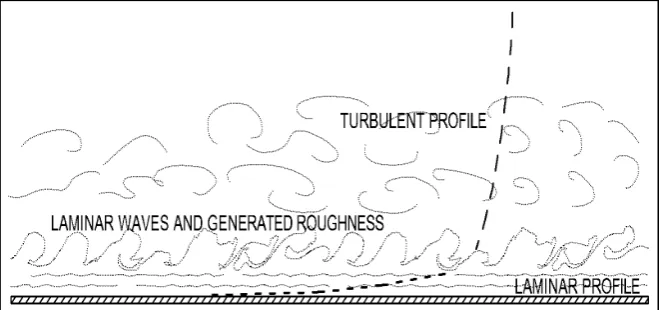
From observations of the sea being ruffled by the wind, Lord Kelvin [11] de-scribed the effects of viscosity and relative velocity upon a fluid surface. The movement of one layer of fluid over another causes a boundary disturbance commonly known as the Kelvin-Helmholtz (KH) instability [11] [12]. This phenomenon is discussed extensively in references by Miles [13], Lamb [14] and others. Figure 1 illustrates an assumed bulk roll-up of the fluid interface be-tween the laminar and turbulent regions similar in form to the KH instability. This figure illustrates flow conditions over a smooth boundary. The presence of boundary roughness elements compound this bulk roll-up as the laminar region moves upward over the roughness elements. This process can be visualized as a wave increases in height when it comes ashore on a beach.
[image:5.595.208.538.559.714.2]The interface between turbulent flow and the surface of the laminar sublayer has to be disturbed and irregular in shape similar to wind moving over waves. Immediately above the laminar sublayer eddies are developing and diffusing throughout the turbulent layer above. As these eddies protrude into the laminar sublayer, the sublayer must speed up or slow down and adjust in depth to ac-commodate this intrusion. Both the turbulent flow and the laminar sublayer are moving in the direction of flow, but the turbulent flow is moving faster than the irregular wave forms on the surface of the laminar sublayer. The wave-like irre-gular shape of the surface of the disturbed laminar sublayer causes a roughness that interferes with the turbulent flow above. We will assume that we can model this roughness effect with the following equation:
(
)
0L 0.13 L L
Z = C H −D (13) where C = adjustment for a moving roughness (0 < C ≤ 1)
HL = height of wave of laminar sublayer above the boundary
DL = average height of laminar sublayer.
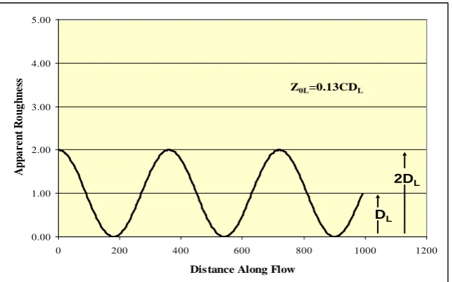
For a symmetrical wave pattern, the maximum value for HL is two times DL, in
which case the lowest part of the wave contacts the boundary (Figure 2). The turbulent flow, thus, contacts the boundary part of the time. It could be argued that there is always a small thickness of laminar flow at the boundary because at the boundary the velocity of fluid movement must be zero. This boundary effect may distort the lower shape of the assumed wave pattern. This distortion should not affect the Z0 value, however, because according to Equation (8) by Abtew et
al. [5], the Z0 is a function of the top half (H-D) of a wave pattern. Interference
by roughness elements slows the turbulent movement and further bunches the laminar flow causing it to amplify the laminar sublayer surface roughness. Because HL is twice DL, Equation (13) reduces to
0L 0.13 L
Z = CD . (14) The fluid roughness changes in proportion to the change in average sublayer depth. Street et al. [15] (1996, page 334) give the following equation for the av-erage depth of the laminar sublayer:
32.8 L
d D
R f
= . (15)
If we substitute the expression for DL from this equation into DL in Equation
(14), we obtain
0L 4.264 d
Z C
R f
= . (16)
[image:6.595.213.536.503.704.2]The friction factor, f, is not independent of R for smooth pipe flow. We can,
Figure 2. Illustration of apparent roughness at the surface of the laminar sublayer.
0.00 1.00 2.00 3.00 4.00 5.00
0 200 400 600 800 1000 1200
Distance Along Flow
A
ppa
re
nt
R
o
ug
hne
ss
2DL
DL
thus, eliminate f in terms of R. We have a couple of ways to estimate f in terms of Reynolds number. The simplest method is to use the Blasius equation [15, page 336]:
0.25 0.316 f
R
= . (17) If we use this relationship to estimate f, Equation (16) reduces to
0L 7.585 0.875 d
Z C
R
= . (18) If we now expand Equation (2) to include both the stationary roughness and the roughness associated with the laminar sublayer, the following is obtained:
0.875 1 0.113 2 log 7.585 33 p d d Cd f R = +
. (19)
This equation reduces to
0.875 1 1 2 log 67.1 3.7 p d C f d R = +
. (20)
This equation is very similar in form to those developed by Swamee and Jain
[7] and Haaland [8]
0.9 1 1 2 log 6.9 3.7 p d f d R = +
. (21)
Based on the success reported by Haaland (1983) of less than three percent error for his results (Equation (21)) and the similarity between Equations (20) and (21), it appears that Equation (20) is a valid model to describe the effects of surface and fluid roughness on the friction factor in pipe flow.
It appears that Haaland [8] adopted the ratio of 6.9/R from the relationship given by Colebrook [4] for smooth pipes over a half century ago,
1 1 1.8 log 6.9 f R =
. (22)
It is interesting that Haaland adjusted the 6.9/R with a power of 0.9, which is very similar to 0.875 obtained in the development of Equation (20).
Equation (20) was tested with data generated using Colebrook’s [4] equation and running enough iterations to obtain no change in the friction factor at the fifth decimal place. A value of C = 0.062 gave the best results. An R2 of 0.9997
points, 33 or 9.2 percent had relative error greater than two percent.
To improve those results, we return to Equation (16) and substitute Equation (6) for f, rather than the Blausius equation. As mentioned earlier, there are al-ternate ways to estimate the friction factor in Equation (16). Although Equation (6) is more complex, it should provide better results. Using Equation 6 to esti-mate the f in Equation (16) produces
( )
0 1
4 0.208ln 3000 4.264 2.3 L R d Z C R R − +
= . (23)
This equation reduces to
( )
0 1
1
4 0.208ln 3000 2.81 L R d Z C R − +
= . (24)
After substitution of this new relationship, Equation (19) becomes
( )
1 1
4 0.208ln 3000
1 0.113 2 log 2.81 33 p R d d Cd f R − + = +
. (25)
which reduces to
( )
1 1
4 0.208ln 3000
1 1 2 log 24.9 3.7 p R d C f d R − + = +
. (26)
This equation was also tested with the generated points from Colebrook’s eq-uation. A value of 0.0618 for C gave the best results. The R2 remained the same
at 0.9997. The number of points with greater than three percent error dropped to zero. The number of points with two or more percent error dropped to three out of the 357 points or 0.84 percent.
Equations (20) and (26) are acceptable and well within the range of scatter reported by Haaland [8] for the experimental data used by Colebrook in his analysis. However, there remains an inherent problem in the development of both equations pertaining to the conceptual basis for f in the square root of the friction factor of the laminar sublayer depth term (Equation (15)). Both the Blausius equation (Equation (17)) and Equation (6), used to compute f in Equa-tions (20) and (26) respectively, are based upon flow passing a smooth boun-dary. To rectify this problem, Equation (26) can be expanded with an adjustment to f. This is done by returning to Equation (16) with the following modification in the development:
adjusted 0 adjusted adjusted 4.264 s L s f f d Z C
f R f f
=
where fs = the friction factor for a smooth boundary
fadjusted = an adjusted friction factor for the actual flow condition.
This equation allows the appropriate friction factor to be used in the laminar sublayer equation by an adjustment factor contained in the parentheses in the above equation. This will be shown to be a function of the relative roughness. An analysis was made to determine C for only smooth boundary values. The result-ing C value became 0.0657. The analysis was repeated for a range of relative roughness values to determine the adjusted best fit value for the product of va-riables contained in parenthesis. This process greatly reduced the error between the Colebrook generated points and the points predicted with Equation (26). Next, the adjusted values relative to the value for a smooth boundary were used to calibrate the adjustment as a function of relative roughness. The relationship is shown in Figure 3. This fraction is an estimate of the square root of the ratio shown in the parenthesis in Equation (27).
The square root ratio was replaced with the equation developed with this analysis:
400
adjusted
0.1e 0.9 4.9
p d
p
s d d
f
f d
−
= + − . (28)
Substitution of this adjustment factor into Equation (26) gives the following:
( )
400
1 1
4 0.208 ln 3000
1 1
2 log
1.64 0.1e 0.9 4.9
3.7
p d
p d
p
R
f d
d d
d
R
−
−
+
=
+ −
+
[image:9.595.211.540.377.713.2]. (29)
Figure 3. Effects of relative roughness on the square root ratio of friction factors.
C Factor Relationship
0 0.2 0.4 0.6 0.8 1 1.2
0 0.01 0.02 0.03 0.04 0.05 0.06
Relative Roughness (dp/d)
( f
s
moo
th
/ f
a
dj
us
te
d
)
0
.5
Equation (29) predicted values matching results from Colebrook’s equation with relatively little error and without the need for iteration. All errors were less than one percent. Most errors were less than 0.3 percent. The R2 improved to
0.99998. This is slightly superior to the R2 of 0.99996 for the correlation of
Haaland’s equation to values from Colebrook’s equation. Based on a reasonable description of the process by which smooth and rough boundaries interact, this equation improves upon the work of Haaland both in accuracy and logic.
4. Discussion
It is interesting to examine Colebrook’s [4] development of the relationship that we cite as Equation (3). On page 139 of his paper, he reports the following:
Other experiments by Nikuradse show that for smooth pipes
1
* 1 10
y
V µ ρ
= . (30)
If we replace friction velocity V* with the form U(f/8)0.5 [15, page 325,
Equa-tion 9.4] and multiple the numerator and denominator on the right side by the diameter of the pipe, we obtain the same relationship as Equation (15) in terms of the friction factor and Reynolds number,
1 8 10
d y
R f
= . (31)
If we now recall that Z0L in Equation (14) and y1 are the same when there is no
roughness, we get the following relationship: 8 1.3 L
d D
C R f
=
. (32) Equation (32) has exactly the same form as Equation (15) given by Street et al. [15, page 334, Equation 9.22]. If we compare the 32.8 from Equation (15) to the value inside the parentheses in Equation (32), and solve for C, a value of 0.0663 is obtained. This value is close to the 0.0657 obtained for the adjusted Equation (26). The relative error between these two estimates of average depth for the la-minar sublayer is between 0.90 and 0.91 percent depending on which one is used as reference. The experimental results of Nikuradse [3] seem to confirm that the laminar sublayer creates a roughness that interacts with the turbulent flow at the intersection of the two flows.
It is obvious that the experiments of Nikuradse produced key information for modeling both the effects of boundary roughness and smooth boundary effects to predict the friction factor. This concept explains why Z0 and Z0L are additive.
Colebrook assumed they were additive to develop his model for the friction fac-tor but did not offer an explanation as to why they are additive. From Equation (8), the additive effect can be explained. The Z0 value in Equation (8) is just the
difference in height of roughness elements and the average height times the con-stant of 0.13. Thus when we add Z0 terms in Equation (7), we are adding the
height of the roughness elements and the difference between the wave height and the displacement height or average height of the laminar sublayer. The total effect is the sum of these two differences.
It has been said that trying to teach something you don’t understand is like trying to describe a place you have never visited. Based on the information pre-sented in this paper, the concepts affecting the friction factor are simple. The friction factor is simply a function of the Z0 or aerodynamic roughness at the
boundary. This roughness is the sum of the physical roughness of the boundary surface and the apparent roughness from turbulence interacting with the lami-nar boundary layer. While the mathematical model to describe this process is messy, the concept is simple and logical.
5. Summary and Conclusions
An attempt has been made to explain how roughness at pipe boundaries affects friction. We acknowledge that a laminar sublayer exists between the region of turbulent flow and the pipe boundary. Furthermore, we use the roughness on the surface of this laminar sublayer to generate a fluid roughness height Z0L.
This roughness in turn affects the velocity profile in the turbulent region simi-lar to the manner in which waves affect the wind profile above a water surface. This concept was used along with relationships presented in the literature to develop mathematical equations for prediction of the friction factor as a func-tion of Reynolds number and relative roughness as used in the development of the Moody Diagram.
Two equations were developed and tested against data generated from the ac-cepted standard for predicting the friction factor in the Moody Diagram. The first used the Blasius equation to estimate the f factor for smooth pipe flow. The second used a more elaborate model to predict f as a function of Reynolds num-ber for the full range of Reynolds numnum-bers in the Moody Diagram. A final equa-tion was developed that accurately predicts the fricequa-tion factor without iteraequa-tion. This equation was achieved by identifying an adjustment factor and relating it to relative roughness. The final equation also eliminates the need to iterate to ob-tain an accurate prediction.
References
[1] Reynolds, O. (1883) An Experimental Investigation of the Circumstances Which Determine Whether the Motion of Water Shall Be Direct or Sinuous and of the Law of Resistance in Parallel Channels. Philosophical Transactions Royal Society Lon-don, 174, 935-982. https://doi.org/10.1098/rstl.1883.0029
[2] Prandtl, L. (1926) Ueber Die Ausgebildete Turbulenz. Proceedings 2nd Internation-al Congress Applied Mechanics, Zurich, 12-17 September 1926, page 62.
[3] Nikuradse, J. (1933) Stromungsgesetze in Rauhem Rohren. (Laws of Turbulent Pipe Flow in Smooth Pipes.) VDI-Forschungsheft: Germany) 361. (in German) (Trans-lated in NACA Tech. Memo. No. 1292, 1050).
Insti-tution of Civil Engineers, 11, 133-156. https://doi.org/10.1680/ijoti.1939.13150
[5] Abtew, W., Gregory, J. and Borrelli, J. (1989) Wind Profile: Estimation of Dis-placement Height and Aerodynamic Roughness. Transactions American Society Agricultural Engineers, 32, 521-527. https://doi.org/10.13031/2013.31034
[6] Moody, L. (1944) Friction Factors for Pipe Flow. Transactions of American Society Mechanical Engineers, 66, 671-678.
[7] Swamee, P., and Jain, A. (1976) Explicit Equations for Pipe-Flow Problems. Journal of the Hydraulics Division-American Society Civil Engineers, 102, 657-664. [8] Haaland, S. (1983) Simple and Explicit Formulas for the Friction Factor in
Turbu-lent Pipe Flow. Journal Fluids Engineering, 105, 89-90.
https://doi.org/10.1115/1.3240948
[9] Gregory, J., Wilson, G., Singh, U., and Darwish, M. (2004) TEAM: Integrated, Process-Based Wind-Erosion Model. Elsevier Environmental Modeling and Soft-ware, 19, 205-215.
[10] Darwish, M. (1998) Process-based Aerodynamic Roughness Model for Evaporation Prediction from Free Water Surfaces. Ph.D. Dissertation, Texas Tech University, Lubbock.
[11] Kelvin, Lord (William Thomson) (1871) Hydrokinetic Solutions and Observations. Philosophical Magazine, 42, 362-377.
[12] Helmholtz, H. (1868) Uber Discontinuirliche Flussigkeits-Bewegungen. Monatsbe-richte der Koniglichen Preussische Akademie der Wissenschaftenzu, Berlin, 215- 228.
[13] Miles, J. (1959) On the Generation of Surface Waves by Shear Flows Part 3. Kel-vin-Helmholtz Instability. Journal Fluid Mechanics, 6, 583-598.
https://doi.org/10.1017/S0022112059000842
[14] Lamb, H. (1945) Hydrodynamics. 6th Edition, Dover Publications, New York. [15] Street, R., Watters, G., and Vennard, J. (1996) Elementary Fluid Mechanics. 7th
Edition, John Wiley & Sons, New York.
Submit or recommend next manuscript to SCIRP and we will provide best service for you:
Accepting pre-submission inquiries through Email, Facebook, LinkedIn, Twitter, etc. A wide selection of journals (inclusive of 9 subjects, more than 200 journals)
Providing 24-hour high-quality service User-friendly online submission system Fair and swift peer-review system
Efficient typesetting and proofreading procedure
Display of the result of downloads and visits, as well as the number of cited articles Maximum dissemination of your research work