Identification of Artificial Neural Network Models for
Three-Dimensional Simulation of a Vibration-Acoustic
Dynamic System
Robson S. Magalhães, Cristiano H. O. Fontes, Luiz A. L. de Almeida, Marcelo Embiruçu Programa de Pós-Graduação em Engenharia Industrial, Escola Politécnica, Universidade Federal da Bahia,
Salvador, Brasil
Email: [email protected], [email protected], [email protected], [email protected]
Received December 18, 2012; revised January 23, 2013; accepted January 30,2013
ABSTRACT
Industrial noise can be successfully mitigated with the combined use of passive and Active Noise Control (ANC) strategies. In a noisy area, a practical solution for noise attenuation may include both the use of baffles and ANC. When the operator is required to stay in movement in a delimited spatial area, conventional ANC is usually not able to ade- quately cancel the noise over the whole area. New control strategies need to be devised to achieve acceptable spatial coverage. A three-dimensional actuator model is proposed in this paper. Active Noise Control (ANC) usually requires a feedback noise measurement for the proper response of the loop controller. In some situations, especially where the real-time tridimensional positioning of a feedback transducer is unfeasible, the availability of a 3D precise noise level estimator is indispensable. In our previous works [1,2], using a vibrating signal of the primary source of noise as an input reference for spatial noise level prediction proved to be a very good choice. Another interesting aspect observed in those previous works was the need for a variable-structure linear model, which is equivalent to a sort of a nonlinear model, with unknown analytical equivalence until now. To overcome this in this paper we propose a model structure based on an Artificial Neural Network (ANN) as a nonlinear black-box model to capture the dynamic nonlinear behave- ior of the investigated process. This can be used in a future closed loop noise cancelling strategy. We devise an ANN architecture and a corresponding training methodology to cope with the problem, and a MISO (Multi-Input Sin- gle-Output) model structure is used in the identification of the system dynamics. A metric is established to compare the obtained results with other works elsewhere. The results show that the obtained model is consistent and it adequately describes the main dynamics of the studied phenomenon, showing that the MISO approach using an ANN is appropriate for the simulation of the investigated process. A clear conclusion is reached highlighting the promising results obtained using this kind of modeling for ANC.
Keywords: Neural Networks; Nonlinear Identification; Dynamic Models; Distributed Parameter Systems;
Vibrate-Acoustic Systems
1. Introduction
Considering performance requirements, requested in many current applications that use mathematical models, the behavior of the most physical phenomena can be repre- sented by linear systems. The procedures for parametric identification for linear systems are well established and show many theoretical and practical results [3,4]. Some systems fail to have their behavior well described by lin- ear models if their frontiers or ranges of values where they are excited are extended. In these cases, it is neces- sary to use a nonlinear model, and the identification of nonlinear systems using neural networks has been at- tracting interest and it has been applied successfully else- where [5-7].
mod-eled. Because of these characteristics, ANNs are being quite well exploited in the identification of nonlinear dynamic systems currently [12], modeling this nonlinear input/output relationship of the identified process, with the variables changing over time. In these cases, the rep- resentation of the dynamics can be characterized through the supplying of the signals set (input and output of the process), which are backward in time at the entrance of the ANN, to include in the modeling the dead time, the memory of the input and the feedback that are associated with the phenomenology of the system, resulting in an input/output representation according to a recurrent ar- chitecture [13,14].
ANN is also being used for applications in Active Noise Control (ANC). Bambang [15] developed an ap- plication in ANC using recurrent neural networks, where the author presents a learning algorithm for recurrent neural networks based on the Kalman filter. The overall structure for the proposed ANC was formulated using two recurrent neural networks: the first neural network is used to model the secondary source of the ANC, while the second network is used to generate the control signal. Chang [16] proposed a structure based on neural net- works in a filtered LMS algorithm, or NFXLMS (Neural- based Filtered-X Least-Mean-Square algorithm), which is associated with a method to prevent the premature saturation of the backpropagation training algorithm us-ing a best adjustment rate. Zhang [17] studied an ANC system with nonlinearities and proposed unconventional structures of neural networks for modeling the nonlinear- ity of the acoustic propagation of the primary source in the system. Bouchard [18] introduced a LMS-based al- gorithm to devise several neural network controllers. The main evaluation criterion used was computation time, aiming at the application of the algorithm in
multichan-nel ANC systems.
We present in this paper a methodology for building an ANN model to estimate the noise level in a certain spatial region subjected to noise emissions from a single vibrating source. The proposed model is designed to run in real-time, providing noise level estimation to be used by an ANC control system.
The neural network is trained to estimate the noise level at any point in the contained space in our acoustic system and uses as variables of input of the spatial coor- dinates of that point and the vibration signal, which is measured at the primary source.
The objective function used in network training is the sum of square errors (difference between the measured value for the noise level and the value predicted by the model in each spatial point). A set of experimental data is chosen for training, using the least squares metric and the obtained neural network is validated through simulations, comparing predictions with another set of data obtained from our experimental platform.
2. Materials and Methods
2.1. Experimental Apparatus and Methodology for Data Collection
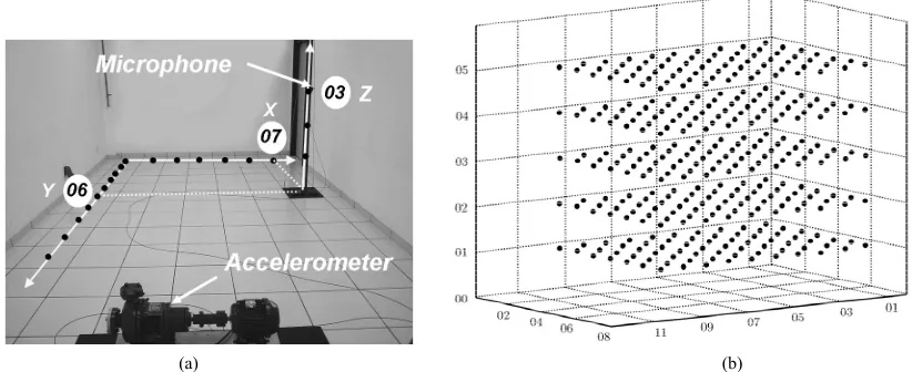
The vibro-acoustic system under study is composed of a centrifugal pump installed in a room (Figure 1(a)). The
centrifugal pump is driven by a simple single-phase in- duction motor and this set is assumed to be our primary source of noise. In this experimental set-up two sensors are used: a fixed ICP (Integrated Circuit Piezoelectric) accelerometer which measures the vibrating signal gen- erated by the primary source and a mobile microphone that measures the sound noise level inside the room, at each point of a previously defined mesh. Figure 2 shows
[image:2.595.90.501.524.692.2]
(a) (b)
Figure 1. Acoustic field mapping generated by a rotating machine operating in a closed room identified by coordinates
, , : , , , . ; , , , . ;
[image:3.595.126.471.85.203.2]
(a) (b)
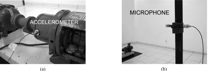
Figure 2. Experimental apparatus: (a) System input, primary source sensor: pump accelerometer
100mV g
signal;(b) System output, passive sensor: microphone
50mV Pa
signal.details of both the accelerometer and the microphone installation. Considering the data collected by the accel- erometer installed in the pump, and varying the position of a microphone per 350 predetermined points in the room (they are identified by its coordinates
, , : 1, 2, ,7 0.44m ; 1, 2, ,10 0.44m
X Y Z X Y ;
and Z 1, 2, ,5
0.44m
), 350 pattern pairs were col- d
lecte up,yp
which repretransm
e used to
sent the dynamic of the vi- bro-acoustic ission between the input signal that comes from the accelerometer (u) and the output signal, which comes from the microphone (y). The collected set of pairs
p, p
,p1, 2, ,350
u y defines the group of
standard that will b t ANN net-
work that can best describe the dynamic of the vibro- acoustic transmission in the proposed experimental plat- form.
train a recurren
2.2. Model Structure: Characteristics of the Used
Since R Ns have been used to model Neural Network
osenblatt [19], AN
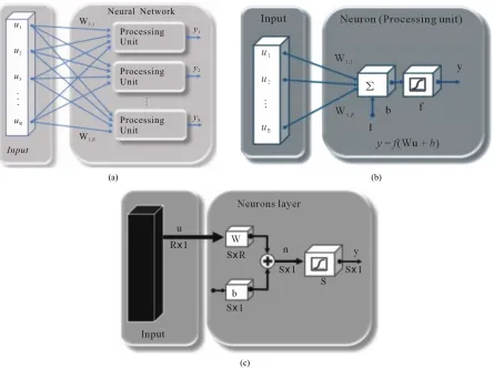
and simulate nonlinear systems of diverse nature in digi- tal computers or in hardware boards. According to Masson [20], and expressed in Figure 3(a), the topology
of an artificial neural network can be expressed through a directed graph characterized by a set of vertices, a set of directed arcs and a set of weights to these arcs
W . Each vertex in the graph represents a processing unit. A processing unit has u u1, , ,2 uR inputs. Based on theseinputs and the set of syn ghts, W1,1, ,WS R, , the
neurons are evaluated, generally throu tion function applied to a weighted sum of inputs using the synaptic weights as weighting factors [20]. A network with a single layer having S neurons with an arbitrary activation function and with R inputs is shown in detail in Figure 3, which also illustrates its processing unit
(neuron). Neural networks frequently have one or more hidden layers of sigmoid neurons (for example, tansig or logsig) [21-23] following by an output layer of linear neurons. If a two-layer network is considered, we have:
one hidden layer with SI sigmoid neurons with biase
aptic wei
gh an activa
s
by a linear
ber of neurons (SI) in the
hi
b1 which are associated with each neuron;
one layer with SL output neurons activated
function with biasesb2, which are associated to each neuron.
By using a sufficient num
dden layer of a two-layer network it is possible to ap- proximate any function with a finite number of disconti- nuities within an accuracy that is arbitrarily specified [24,25]. This structure is shown in Figure 4 and it can be
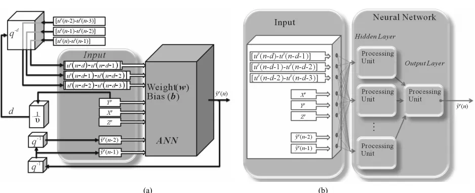
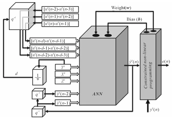
used as a universal approximator of functions. The rep- resentation of the system dynamics was characterized through the use of the set of input and output of the process (u and y), backward in time, placed in the ANN´s input, as mentioned previously [13,14] and shown in
Figure 5, which also illustrates the internal structure of
the adopted ANN (an intermediate layer and an output layer). In this figure u n
is a sampling of the input signal at time n, y n
the sampling of the output signal at time n, d is the delay (dead time) of the system output, relating to the input u and q is the forward shift operator. The scheme shown in Figure 4 (general ap-proximator of functions) is used, therefore this ANN is able in principle to approximate any function with a fi- nite number of discontinuities using a sufficient number of neurons
is
SI in the hidden layer.The chosen orders for u and y in Figure 5 are the same
as those adopted in the work of Magalhaes [1] that pre- sents an extensive discussion about the dynamic behavior expected for the acoustic problem studied. Thus, consid- ering that the X, Y and Z coordinates of any point in a room are also inputs to the net work (in this case static and therefore of zero order), we can conclude that the dynamic ANN to be configured to estimate the y nˆp
acoustic pressure in an arbitrary spatial position ha entries. For the time delay the same procedure of Magalhaes [1] is adopted, where d is calculated on a theoretical basis, using sound velocity (v) and longitude- nal distance (Y) between primary source and the grid measurement point.
(a) (b)
[image:4.595.77.522.84.417.2](c)
Figure 3. Neural network with a single layer (a), its processing unit (b) and its diagram (c).
Figure 4. Structure of a network with one hidden layer with sigmoid function and an output layer with linea function
(func-Magalhaes [1] presented the development of the ma- ch
the identified models was applied. This procedure re- r
tion universal approximator).
ine room transfer function (Machine-Room Transfer Function—MRTF), which simulates the acoustic trans- mission between the primary source and a receiver in a room, including the spatial distribution of 350 MRTFs (Machine-Room Transfer functions) and a total of 1750 parameters. In order to reduce the number of parameters of the models used to describe the spatial behavior of the acoustic system, an interpolation process on a subset of
[image:4.595.125.473.449.587.2][image:5.595.65.534.78.269.2]
(a) (b)
[image:5.595.45.545.315.473.2]Figure 5. ANN structure ( al structure adopted (b).
Table 1. Comparison of the Euclidean norm of the errors.
Errors Euclidean Norm (Pa2):
Average Minimum Maximum Number of parameters
long-range prediction) (a) and details of the intern
Models:
Euclidean norm of the output signal 11.8 4.9 21.6 - Identified ARX without delay (350 MRTFs) 1750
s)
7.3 3.6 15.8
Identified ARX with delay (350 MRTFs) 7.1 4.1 13.3 1750
Interpolated ARX with delay (27 MRTF 9.3 4.6 20.8 135
Interpolated ARX with delay(18 MRTFs) 9.8 4.6 22.0 90 Interpolated ARX with delay(9 MRTFs) 10.8 5.0 19.9 35 Interpolated ARX with delay(4 MRTFs) 11.0 5.0 19.9 20
ANNwith delay 9.3 4.9 16.7 80
llows future implementation of this model structure in
aring the present structure w
(1)
where R is the number of network in I
in hidden layer was equal to 8.
er Estimation: Training of the Recurrent Network
neces-
sary was for-
a
control systems in real-time. For the purpose of comp
ith that obtained in the work of Magalhaes [1], the maximum number of parameters for the current network was established to be less than 135, the number of pa- rameters adopted by Magalhães and coworkers. This assumption is supposed to produce no hammering in the quality obtained for the proposed model, nor in the com- parison outcome with the previous model. The total number of parameters in an ANN (Figure 4) with one
hidden layer (intermediate) and one neuron in the output layer is given by:
Np R SI 2 SI1
puts and S is the number of neurons of the hidden layer. In this work,
80 p
N was adopted in order to keep the resulting of parameters less than 135, as stated earlier. With the input layer defined according to the Figure 5
R8
and using Equation (1), the number of neurons2.3. Procedure for Paramet
number
Once the network topology is characterized, it is to establish the training procedure, which
mulated through the optimization procedure shown in
Figure 6, where e n
represents the simulation error.Thus, the training of the network was formulated as a general problem of nonlinear optimization with con- straints [27,28]:
minf x
subject to0, 1, ,
0, 1, ,
x
i e
i e
G x i m
G x i m m
(2)
where x is the vector ofparametersof length n, f x
value, and is the objective function, which gives a scalar
the vector function G x
gives a vector of mFigure 6. Recurrent ANN training (long-range prediction).
ontaining the values of equalities and inequalities con- c
straints which are evaluated at x. Constraints are usually used to achieve certain desired properties for the network or to restrict the search region to avoid convergence problems. For both the topology and the experimental data used in our ANN model, no constraints were neces- sary because the optimization algorithm behaved smoo- thly in most of the runs.
The solutions of the Khun-Tucker (KT) [29], equa- tions are the basis for many nonlinear programming al- gorithms. The methods that use these algorithms are commonly referred to as Sequential Quadratic Program- ming (SQP). SQP methods, described in [30-32] works, offer a good method for solving the problem of ANN dynamic optimization. A SQP overview can be found in [33].
The training was performed using MATLAB®. The
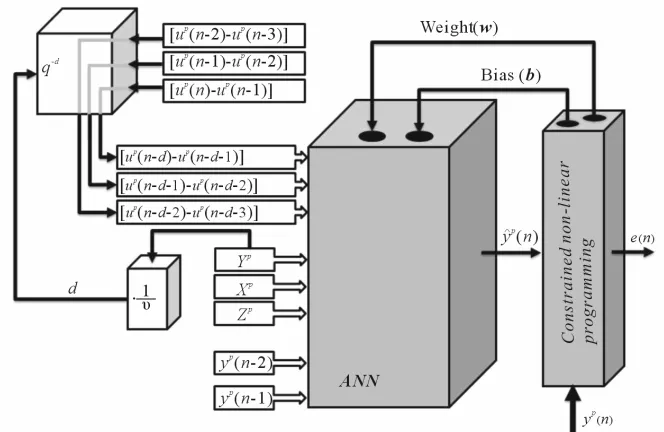
availability of a good initial estimate is an important req- uisite for success in solving these problems. In this case, an initial guess was used to train the model according to the scheme shown in Figure 7 which consists of an iden-
tification procedure based on one-step ahead prediction. A set of patterns was used made up of pairs that were collected in the experiment
p, p
,p1, 2, ,350
u y
which defines the input vector f
to Equation (3). A network able to do one-step ahead prediction is not the final network of interest rather a dynamic model able to perform long-range prediction is desirable (Figure 6). However, the one-step ahead pre-
diction network (Figure 7) provides a good initial esti-
mate for the optimization procedure shown in Figure 6.
Thus, the parameters (weights and bias) obtained through
training (Figure 7) are used as initial condition for the
optimization procedure defined for the recurrent ANN training (long-range prediction) (Figure 6). In the opti-
mization procedure used here (Figures 6 and 7), the ob-
jective function, which is used in the networks training, is the average of the square root of the sum of square errors (difference between the measured value and the value that was estimated by the model for each output value, which is given by
or each time n, according
the one-step ahead optimization procedure for the ANN
e n ), for n1, ,390 .
350
1
p p
p p
Input
2 1
p p
1
1 2
2 3
p
p
p
p
p
p
u n d u n d
u n d u n d
n d
u n u
n
d X Y Z y n
y n
(3)
3. Results and Discussion
As stated earlier, it is necessary to establish a metric his met- in the determination of (criterion) to be used in the objective function. T
ric can have a decisive influence
[image:6.595.315.540.480.620.2]
Figure 7. ANN training (one-step ahead prediction).
is commonly used in the treatme
rder to obtain an objective function that gives the dis- nt of causal events in o
tance of functional responses (responses of the models) in relation to its target profile (experimental output). Euclidean distance is also commonly called the error vector norm (EVN) and is given by:
2, Mod , Exp ,
TP
s TD s n s n
EVN
y y1
, 1, , n
s SP
(4)
for the time domain, and by:
2, Mod ,
s FD s
EVN
Y YExp ,1
2π 1 1 Mod , Mod ,
1
2π 1 1 Exp , Exp ,
1
, 1, ,
e , 1, ,
e , 1, ,
2 π 1 TP
s k
TP
j k n TP
s s n
n TP
j k n TP
s s n
n
s SP
Y y k TP
Y y k TP
k h k TP
(5)for the frequency domain, where SP and TP are the numbers of points in space and in time, respectively, y
ed by the objective f tio
ons, obtaining equivalent models. Here, for the purpose of numerical comparison between
the best and the worst results of the models in th
hted:
agalhaes [1], the maxi-
y reduction superior to
of the error norm to higher values compared to the and Y are the outputs in the time and in the frequency
domains respectively, the subscripts Mod and Exp refer to the model and to the experimental output respectively, the subscript s defines a specific spatial position, k and ω
are the discrete time and frequency, respectively, the subscripts TD and FD refer to the domains of time and frequency, respectively, and h symbolizes the functional relationship between ω and k.
In the optimization procedure used here (Figures 6
and 7), both metrics establish unc- this takes the average, minimum or maximum values
ns described in Equations (4) and (5) were tested, as
the different modeling approaches, Equation (4) was as- sumed.
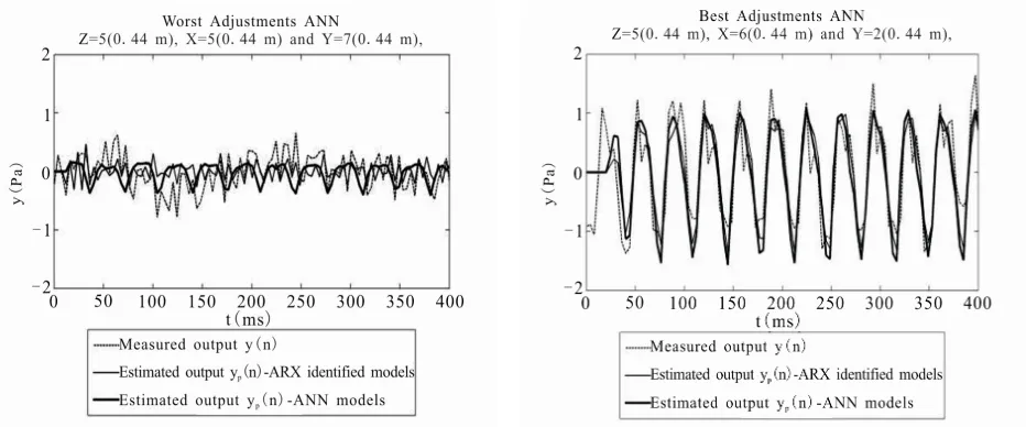
The resulting models were used to predict the dy- namic and spatial behavior of the system´s output signal (acoustic power measured by microphone). From Fig-ures 8-10
well as their combinati
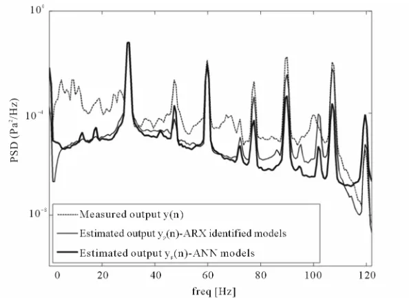
e estimation of the output signal for plans Z=1, 3 and 5 can be seen, as well as a qualitative comparison with estimated results with the models that were obtained in the work of Magalhaes [1]. It can be seen that even the worst results with the ANN models provide an adequate dynamic representation of the experimental data, captur- ing the main trends of the system behavior, although the amplitudes at higher frequencies have a strong attenua- tion, as can be seen in Figure 11, which shows the aver-
age PSD (Power Spectral Density) for 350 mesh points. The ANN model provides a good system dominant dy- namic description (PSD peaks), where most of the signal energy is concentrated).
Table 1 compares the result of the model structure
proposed in this work with the results obtained by Magalhaes [1]. Based on these results, the following conclusions may be highlig
Smaller errors are obtained when considering the de- lays in each XZ plane to identify the models in the various grid points collected;
According to the results of M
[image:7.595.59.291.408.572.2]
Figure 8. Best and worst adjustments for plane Z = 1 × (0.44 m): time response of ARX identified models and ANN models.
[image:8.595.66.536.306.490.2]
Figure 9. Best and worst adjustments for plane Z = 3 × (0.44 m): time response of ARX identified models and ANN models.
.
Z 5 0 44m
[image:8.595.67.533.521.715.2]Figure 11. Average PSD for the output.
respective Euclidean norm values of the experimental signal (the objective function, which is used in the net-works training, is the average of the square root of the sum of square errors);
The ANN model performed equivalent to the ARX model (27 MRTFs, 135 parameters), with the advan- tage that it used fewer parameters (80 parameters).
4. Conclusion
This paper presented the development of an Artificial Neural Network (ANN) to describe the vibrate-acoustic transmission between a primary source of noise and a receiver in a room. The obtained dynamic ANN model captured the main dynamics of the system and performed equivalent to the performance presented by an ARX- interpolated model [1]; however, with fe
onsidering that these two model struct
ber of model parameters, requiring fort to simulate the outputs of
models with low computational cost, and therefore mod-els with increased number of neurons would not satisfy this requirement.
5. Acknowledgements
The authors acknowledge CAPES and CNPq (Brazilian federal research agencies) for their financial support.
REFERENCES
[1] R. S. Magalhaes, C. H. O. Fontes, L. A. L. Almeida, M. Embirucu and J. M. C. Santos, “A Model for Three- Dimensional Simulation of Acoustic Emissions from Rotating Machine Vibration,” Journal of the Acoustical Society of America, Vol. 127, No. 6, 2010, pp. 3569-3576. doi:10.1121/1.3425736
es, C. O. H. Fontes, L. A. L. Almeida, J. M. M. Embirucu, “A Model for Three-Di- wer parameters.
ures have a dif-C
ferent number of parameters, the dynamic ANN model demonstrated better adherence to the experimental data, providing the smallest variance errors in the estimate of the system output (Table 1). It is possible to further
im-prove the performance of the dynamic ANN model, al-though this requires a change in the proposed structure for this model, such as increasing the number of neurons in the hidden layer. Strategies like this, however, would increase the num
greater computational ef
the system. We need models that have the ability to simulate (qualitatively and quantitatively) the dynamics of vibrate-acoustic systems because the ultimate goal of this research project is the development of three-dimen- sional models for use in the construction of systems to Active Noise Control (ANC). In this case, we also need
[2] R. S. Magalha C. Santos and
mensional Simulation of Acoustic Emissions from Rota- ting Machine Vibration,” Composites 2009, 2nd ECCO- MAS Thematic Conference on the Mechanical Response of Composites, London, 1-3 April 2009.
[3] B. O. Kachanov, “Symmetric Laplace Transform and Its Application to Parametric Identification of Linear Sys- tems,” Automation and Remote Control, Vol. 70, No. 8, 2009, pp. 1309-1316. doi:10.1134/S0005117909080049 [4] E. L. Hines, E. Llobet and J. W. Gardner, “Electronic
Noses: A Review of Signal Processing Techniques,” IEEE Proceedings—Circuits Devices and Systems, Vol. 146, No. 6, 1999, pp. 297-310.
doi:10.1049/ip-cds:19990670
[6] J. Madar, J. Abonyi and F. Szeifert, “Genetic Program- ming for the Identification of Nonlinear Input-Output Models,” Industrial & Engineering Chemistry Research, Vol. 44, No. 9, 2005, pp. 3178-3186.
doi:10.1021/ie049626e
[7] V. Prasad and B. W. Bequette, “Nonlinear System uction Using Artificial Neural
d Chemical Engineering, Vol Iden-
. tification and Model Red
Networks,” Computers an
27, No. 12, 2003, pp. 1741-1754. doi:10.1016/S0098-1354(03)00137-6
[8] S. M. Siniscalchi and C.-H. Lee, “A Study on Integrating Acoustic-Phonetic Information into Lattice Rescoring for
Automatic Spe h Communication
Vol. 51, No. 11,
, ech Recognition,” Speec
2009, pp. 1139-1153. doi:10.1016/j.specom.2009.05.004
[9] L. Yu and J. Kang, “Modeling Subjective Evaluation of Soundscape Quality in Urban Open Spaces: An Artificial Neural Network Approach,” Journal of the Acoustical So- ciety of America, Vol. 126, No. 3, 2009, pp. 1163-1174. doi:10.1121/1.3183377
[10] A. Dariouchy, E. Aassif, G. Maze, D. Decultot and A. Moudden, “Prediction of the Acoustic Form Function by Neural Network Techniques for Immersed Tubes,” Jour- nal of the Acoustical Society of America, Vol. 124, No. 2, 2008, pp. 1018-1025. doi:10.1121/1.2945164
[11] A. Saxena and A. Saad, “Evolving an Artificial Neural Network Classifier for Condition Monitoring of Rotating Mechanical Systems,” Applied Soft Computing, Vol. 7, No. 1, 2007, pp. 441-454. doi:10.1016/j.asoc.2005.10.001 [12] A. C. Tsoi and A. D. Back, “Locally Recurrent Globally
Feedforward Networks—A Critical-Review of Architec- tures,” IEEE Transactions on Neural Networks, Vol. 5, No. 2, 1994, pp. 229-239. doi:10.1109/72.279187
ra, “Control Of Nonlinear [13] A. U. Levin and K. S. Narend
Dynamic-Systems Using Neural Networks—Controllabi- lity and Stabilization,” IEEE Transactions on Neural Net- works, Vol. 4, No. 2, 1993, pp. 192-206.
doi:10.1109/72.207608
A. U. Levin and K. S. Narendra, “Contro o
[14] f Nonlinear
Dynamical Systems Using Neural Networks. II. Obser- vability, Identification, and Control,” IEEE Transactions on Neural Networks, Vol. 7, No. 1, 1996, pp. 30-42. doi:10.1109/72.478390
R. T. Bambang, “Adjoint
[15] EKF Learning in Recurrent Neu-
ral Networks for Nonlinear Active Noise Control,” Applied Soft Computing, Vol. 8, No. 4, 2008, pp. 1498-1504. doi:10.1016/j.asoc.2007.10.017
[16] C.-Y. Chang and F.-B. Luoh, “Enha Noise Control Using Neural-Based Filt
ncement of Active ered-X Algorithm,”
Journal of Sound and Vibration, Vol. 305, No. 1-2, 2007, pp. 348-356. doi:10.1016/j.jsv.2007.04.007
[17] Q.-Z. Zhang, W.-S. Gan and Y. Zhou, “Adaptive Recur- rent Fuzzy Neural Networks for Active
Journal of Sound and Vibration, Vol. 296, No. 4-5, 2006, Noise Control,” pp. 935-948. doi:10.1016/j.jsv.2006.03.020
[18] M. Bouchard, “New Recursive-Least-Squares Algorithms for Nonlinear Active Control of Sound and Vibration Using Neural Networks,” IEEE Transactions on Neural Networks, Vol. 12, No. 1
doi:10.1109/72.896802
[19] F. Rosenblatt, “The Perceptron—A Probabilistic Model for Information-Storage and Organization in the Brain,”
Psychological Review, Vol. 65, No. 6, 1958, pp. 386-408. doi:10.1037/h0042519
[20] E. Masson and Y. J. Wang, “Introduction to Computation and Learning in Artificial Neural Networks,” European Journal of Operational Research, Vol. 47, No. 1, 1990, pp. 1-28. doi:10.1016/0377-2217(90)90085-P
[21] M. Nikravesh, A. E. Farell and T. G. Stanford, “Model Identification of Nonlinear Time Variant Processes via Artificial Neural Network,” Computers & Chemical Engi- neering, Vol. 20, No. 11, 1996, pp. 1277-1290.
doi:10.1016/0098-1354(95)00245-6
[22] J. X. Zhan and M. Ishida, “The Multi-Step Predictive Control of Nonlinear SISO Processes with a Neural Mo- del Predictive Control (NMPC) Method,”
Chemical Engineering, Vol. 21, No. 2, 1997, pp. 201-210. Computers & doi:10.1016/0098-1354(95)00257-X
[23] K. Narendra and K. Parthasarathy, “Identification and Con- trol of Dynamical Systems Using Neural Networks,” IEEE Transactions on Neural Networks, Vol. 1, No. 1, 1990 4-27.
, pp. 02
doi:10.1109/72.802
n-
[24] A. J. Meade and H. C. Sonneborn, “Numerical Solution of a Calculus of Variations Problem Using the Feed- forward Neural Network Architecture,” Advances in E gineering Software, Vol. 27, No. 3, 1996, pp. 213-225. doi:10.1016/S0965-9978(96)00029-4
[25] R. R. Selmic and F. L. Lewis, “Neural-Network Appro- ximation of Piecewise Continuous Functions: Application to Friction Compensation,” IEEE Transactions on Neural Networks, Vol. 13, No. 3, 2002, pp. 745-751.
doi:10.1109/TNN.2002.1000141
[26] N. Takagi and S. Kuwahara, “A VLSI Algorithm for Computing the Euclidean Norm of a 3D Vector,” IEEE Transactions on Computers, Vol. 49, No. 10, 2000, pp. 1074-1082. doi:10.1109/12.888043
[27] L. T. Biegler and I. E. Grossmann, “Restrospective on Optimization,” Computers and Chemical Engineering, Vol. 28, No. 8, 2004, pp. 1169-1192.
doi:10.1016/j.compchemeng.2003.11.003
[28] P. E. Gill, W. Murray and M. A. Saunders, “A Practical Anti-Cycling Procedure for Linearly Constrained Optimi- zation,” Mathematical Programming, Vol. 45, No. 3, 1989, pp. 437-474. doi:10.1007/BF01589114
[29] O. A. Brezhneva, A. A. Tret’yakov and S. E. Wright, “A Simple and Elementary Proof of the Karush-Kuhn-Tucker Theorem for Inequality-Constrained Optimization,” Opti- mization Letters, Vol. 3, No. 1, 2009, pp. 7-10.
doi:10.1007/s11590-008-0096-3
[30] M. C. Biggs, “Convergence of Some Constrained Mini- mization Algorithms Based on Recursive Quadratic Pro- gramming,” Journal of the Institute of Mathematics and Its Applications, Vol. 21, No. 1, 1978, pp. 67-81. doi:10.1093/imamat/21.1.67
[31] S. P. Han, “Globally Convergent Method for Nonli- near-Programming,” Journal of Optim
Applications, Vol. 22, No. 3, 1977, pp
ization Theory and
doi:10.1007/BF00932858
[32] R. P. Ge and M. J. D. Powell, “The Convergence of Variable-Metric Matrices in Unconstrained Optimization,”
Mathematical Programming, Vol. 27, No. 2, 1983, pp. 123-143. doi:10.1007/BF02591941
[33] W. Hock and K. Schittkowski, “A Comparative Perfor- mance Evaluation of 27 Non-Linear Programming Codes,”
Computing, Vol. 30, No. 4, 1983, pp. 335-358. doi:10.1007/BF02242139
[34] P. E. Danielsson, “Euclidean Distance Mapping
puter Graphics and Image Processing
,” Com-