The predictability of asset returns in the BRICS countries: a nonparametric approach

Munich Personal RePEc Archive

The predictability of asset returns in the

BRICS countries: a nonparametric

approach

Muteba Mwamba, John Weirstrass and Webb, Daniel

University of Johannesburg, department of economics, University of

Johannesburg, department of economics

5 July 2014

The predictability of asset returns in the BRICS countries:

a nonparametric approach

J.W. Muteba Mwamba

_{and Daniel Webb}

Abstract

One of the earliest and most enduring questions of financial econometrics is the predictability of financial asset prices. In this article, stock market data from Brazil, Russia, India, China and South Africa are used to assess the out-of-sample performance of the ARMA(1,1)-GARCH(1,1) and Non-parametric kernel (Epanechnikov) regression models. The results reveal that the non-parametric kernel regression model outperforms its non-parametric rival based on the predicted mean square error (PMSE), Diebold-Mariano criterion, Mean-Absolute Deviation (MAD) and Variance statistics. These results confirm those found previously by other researchers whereby non-parametric forecasting models outperform parametric models in the short-term forecasting horizon.

1 _{Corresponding author. University of Johannesburg, Department of economics and Econometrics}

Email: [email protected]

1

Introduction

For many years economic researchers have studied whether a level of predictability exists in financial markets. The fundamental role of the economy is the allocation of capital as efficiently as possible (Wurgler, 1999). An efficient allocation of capital would be where sectors are expected to have high returns while avoiding sectors with poor prospects.

Being able to predict financial asset prices correctly would allow investors flexibility in the portions they choose to invest in when diversifying their portfolio(s), and thus enable them to create abnormal returns. Although prices are observed in financial markets, the majority of the literature has focused on returns. Returns have been used in research studies instead of the actual observed prices as they tend to be stationary, whilst prices are non-stationary. Fama (1965), Bollerslev (1987), Mandelbrot (1963) and Pesaran and Timmermann (1995) are amongst those that have used various techniques in an attempt to predict the returns in financial markets.

This argument, whether asset returns are predictable, is contradictory to the efficient market hypothesis (EMH). The EMH, as developed by Eugene Fama (1965), is a theory which has dominated the economic profession since its inception and remains a fundamental pillar of Modern Economics. The EMH is of the view that the prices for a financial asset incorporate all available information. The EMH is founded on the assumption that all investor reactions are random and follow a normal distribution (Fama, 1965). When new information is released into the market, some investors overreact and others under-react, creating a net effect on the financial asset prices. In so doing, this creates the environment in which no consistent abnormal profits can be realised.

When analysing the time-series of share prices, it is noted that they display no serial

dependency or “patterns” which leads to the conclusion that a model best equipped to predict

asset returns would be that of a Random Walk process (Fama and Schwert, 1977). However, the time series of a Random Walk model are not random, but the differences from one period to the next are random. It is only after careful analysis that a high degree of positive correlation between the degree of trending and the length of time studied exists, according to Granger and Morgenstern (2007). As proven in Lo and Mackinlay (1999), the stock prices in the short-run exhibit some predictable momentum which leads to the conclusion, in practice, that stock prices do not always behave as true Random Walks and that a degree of predictability does exist.

The different levels of information, public and private, impact financial asset returns with varying magnitude. Events such as an oil shock, a large corporate bankruptcy or the political downfall of a sovereign are typical examples of events that could have a large impact on the financial asset returns. The fat tails so typically found in financial asset returns distributions are where these extreme events tend to occur. It is due to this that that the failure of the normality distribution is more the expectation than the exception when dealing with financial returns.

2

Ultimately, emerging economies are best suited when exploiting financial markets to achieve

“excess” returns. The higher volatilities experienced in these markets create the ideal environment for a predictable element. Conditional asset pricing models, on average, fail to accurately price emerging market assets and capture the time variation in expected returns (Harvey, 1995). When specifically focusing on the applications of parametric and semi-parametric methods to assess the predictability in stock returns, Bollerslev, Chou and Kroner (1992) provide more than a hundred references, all with differing levels of predictability.

Nonparametric methods relax the linearity assumption made by so many parametric methods, such as the infamous Random Walk model. Nonparametric methods apply no assumption to the functional form, i.e. allow the distributions to remain intact instead of forcing them into a Gaussian distribution. The benefits of relaxing the distribution assumption, is ultimately allowing the data to follow its natural, or inherent, distribution. Being able to model asset returns in this way, would theoretically only increase the predictive accuracy of the models.

For this reason, applying nonparametric regression techniques to emerging market economies, specifically the major trading partners, are expected to yield positive results.

3

Methodology

As stated earlier, this paper compares the forecasting ability of the ARMA(1,1)-GARCH(1,1) and non-parametric kernel regression models. The specifications for each of the respective models are described below:

1.1 ARMA(1,1)-GARCH(1,1) model

It has been shown that South Africa doesn’t display evidence of long memory in the equity market (Jefferis and Thupayagale, 2008). It is due to this fact, and to remain consistent across the countries in the BRICS trade union, that the ARMA(1,1) specification was selected. Due to the low levels of skewness, indicating that asymmetry is perhaps not as prominent within the BRICS countries, a standard GARCH(1,1) model following a student-t distribution has been selected.

The ARMA-GARCH model specification is as follows:

(1)

(2)

(3)

where is the stock market return, is the time-varying conditional variance with and

being the coefficient of the AR(1) and risk premium parameters respectively in the mean

equation. The coefficients and are the intercept and the coefficient of the last period

forecast variance respectively. The error term, is a Gaussian innovation with zero mean and

time varying conditional variance ( ).

1.2 Non-parametric kernel regression model

The non-parametric kernel regression model has the benefit that the distribution of the function is not specified. This benefit allows the data to keep the distribution which they already have, instead of forcing it to have a Gaussian form. This means that extreme market events will be better captured and if the data are allowed to speak for themselves, the chances of better prediction are only increased.

Similar to parametric regression, a weighted sum of the observations is used to obtain the

fitted values. In this setting, equation 1 can be re-written in the form:

(4)

with an unknown differentiable function of the independent variable of polynomial degree

4

independent variable of polynomial degree with optimal bandwidth . The kernel density

estimator of the unknown distribution has the form:

(5)

where has the bandwidth (neighbourhood) for a given data point, and is the sum of weights

assigned to each data point which satisfies the following three criteria:

(a)

(b)

(c)

The criteria above ensure that is itself a density and symmetric about zero. It is important

to note that the bandwidth, , acts as a scaling factor in determining the spread of the kernel. A

list of popular kernel functions that are widely used today include the following; Gaussian kernel, Biweight kernel, uniform kernel.

The function selected in this model is the Epanechnikov kernel with the following form:

(6)

However, as mentioned earlier the form of the kernel is not as important as the optimal bandwidth that is selected but the combination of the two should aim to reduce the integrated mean square error (IMSE) function. From calculus variations in solving the minimising of the

IMSE of the kernel estimator, the Epanechnikov kernel has been selected.

The bandwidth of the kernel is known as the “free parameter” which allows for a strong

influence on the resulting distribution (Nadaraya, 1964). The most common optimality criterion

used to select and estimate this parameter is the mean integrated squared error (MISE) and

has the following functional form:

(7)

The above form can be broken down into the variance and bias (using the Taylor expansion formula) within the kernel density estimator, with the respective forms:

(8)

(9)

5

(10)

where and

The optimal bandwidth for the kernel can be obtained by minimizing the function with

respect to as follows:

(11)

This optimal bandwidth corresponding to the optimal kernel density function was first suggested by Epanechnikov (1967) and is given in equation 6.

Estimating the conditional mean and volatility of the nonparametric class of models differs from the parametric counterparts in two ways, namely:

1. The classical Autoregressive (AR) model assumes that a linear dependence exists between the current and previous stock returns, whereas nonparametric models assume a non-linear relationship between stock returns.

2. The classical GARCH models, used to account for volatility, assume the volatility to be normally distributed and symmetrical. (Mwamba, 2011)

From equation 4, the estimator of the conditional mean is given by:

(12)

Determined by fitting the polynomial of degree (equation 13)with the following form and using

the least square cross validation technique to yield equation 14:

(13)

(14)

Setting the polynomial to the 0th– _{degree, the resulting estimator is obtained:}

(15)

The above estimator is also known as the Nadaraya-Watson estimator (Watson, 1964) and

occurs when the polynomial is assigned the 0th_{-degree polynomial. When the polynomial is}

assigned the first degree, the estimator takes the following form, known as the local linear estimate:

6

Similarly, the conditional volatility from equation 4 can be determined by first computing the residuals from the conditional mean:

(17)

Using equation 17, fitted with the polynomial function specified in equation 13 to obtain the following estimator of volatility:

(18)

Setting the polynomial to the 0th_{-degree, the resulting estimator is as follows:}

(19)

Once again, if the polynomial is assigned the first degree the local linear estimate is obtained for the conditional volatility

Data and Empirical Estimation

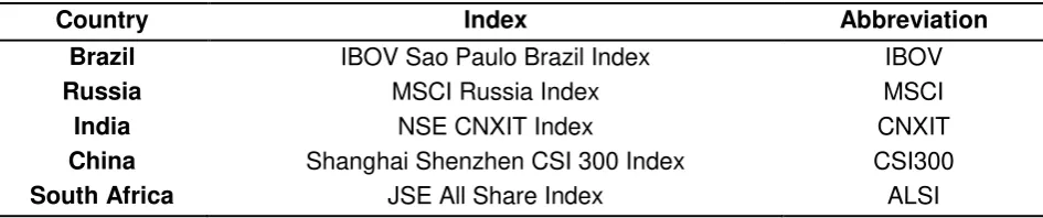
The data used in the analysis of this paper makes use of the major indexes from the BRICS countries and are described in Table 1 below:

Table 1 - BRICS countries with major financial index

Country Index Abbreviation

Brazil IBOV Sao Paulo Brazil Index IBOV

Russia MSCI Russia Index MSCI

India NSE CNXIT Index CNXIT

China Shanghai Shenzhen CSI 300 Index CSI300

South Africa JSE All Share Index ALSI

The data collected for each index were the daily closing prices for the period from January 2006 until July 2013. This specific time-series was selected as it includes the turmoil experienced in the financial markets, resulting from the Global Financial and Sovereign Debt crisis. Due to the prices of the financial time-series being non-stationary, the time-series of returns for each index was calculated based on the following approach:

The first difference of the logarithm of each of the indexes is used to create a time series of returns for the respective indexes, as per the following formula:

where and are the return and stock price respectively for period

7 1.1.1 Shapiro-Wilk

This test makes use of the null hypothesis that a sample came from a normally distributed population. The test statistic is determined as follows:

where is the i-th order statistic and is the sample mean. The constants are given by

where are the expected values of the order statistics of

random variables sampled from the standard Gaussian distribution. The W statistic is

positive and less than or equal to one. Small values of the W statistic lead to the rejection of normality while being close to one indicates normality of the data, but this statistic is sensitive to sample size.

1.1.2 Kolmogorov-Smirnov (K-S)

This is a nonparametric test for the equality of continuous, one dimensional probability distributions that can be used to compare a sample with a reference probability distribution. It is a step function that takes a step of height 1/n at each observation. The downfall of this test, in that it applies to continuous distributions, means that it appears more sensitive near the centre of the distribution than at the tails (Peng and Lilly, 2004). The null hypothesis for this test is that the sample is normally distributed. The empirical distribution function is as follows:

where is the indicator function, equal to 1 if and equal to zero otherwise.

1.1.3 Cramer-von Mises

The Cramer-von Mises criterion is used for judging the goodness of fit of a cumulative distribution function to an empirical distribution function. This test is an alternative to the Kolmogorov-Smirnov test and is defined as follows:

where is the cumulative distribution and is the empirical distribution function.

For the purpose of this paper, the cumulative distribution function will be that of the respective index whilst the empirical distribution function will be parameterised according to a standard Gaussian distribution. By deduction then, if the statistic value is large positive then the hypothesis that the data came from the normal distribution can be rejected.

1.1.4 Anderson-Darling

8

The test statistic, based on the squared difference, places greater emphasis on the tails than does the Kolmogorov-Smirnov (K-S).

The test statistic is calculated as follows:

where and with

being the cumulative distribution function and being the hypothesized function (in this case

the normal distribution).

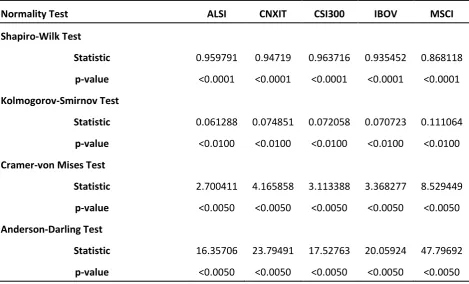
These four tests were applied to all the indexes and their corresponding statistical and p-values are presented in Table 2 below respectively.

Table 2 - Comparison of Normality Tests

Normality Test ALSI CNXIT CSI300 IBOV MSCI

Shapiro-Wilk Test

Statistic 0.959791 0.94719 0.963716 0.935452 0.868118

p-value <0.0001 <0.0001 <0.0001 <0.0001 <0.0001

Kolmogorov-Smirnov Test

Statistic 0.061288 0.074851 0.072058 0.070723 0.111064

p-value <0.0100 <0.0100 <0.0100 <0.0100 <0.0100

Cramer-von Mises Test

Statistic 2.700411 4.165858 3.113388 3.368277 8.529449

p-value <0.0050 <0.0050 <0.0050 <0.0050 <0.0050

Anderson-Darling Test

Statistic 16.35706 23.79491 17.52763 20.05924 47.79692

p-value <0.0050 <0.0050 <0.0050 <0.0050 <0.0050

From the table above, all the p-values were rejected for all the indexes at a 95% confidence level and hence none of the distributions are Gaussian in nature.

Having a stationary time-series, verified by the Augmented-Dickey-Fuller (ADF) test in Table 3 below, the data were then further divided into sample and out-sample datasets. The in-sample dataset will be the training in-sample for the two models, whilst the remaining out-in-sample will be for the forecasting comparisons. The out-sample dataset will cover the last ten (10) observations. The data used within this paper were sourced from Bloomberg. An important assumption was made with respect to public holidays occurring on trading days for the respective indexes. The assumption was that where a public holiday occurs, it was allocated

9 Table 3 - Augmented Dickey-Fuller Stationarity Test

Stationarity Test MSCI IBOV CSI300 CNXIT ALSI ADF Statistic (Lag = 0) -41.192 -44.093 -41.999 -42.505 -42.925

p-value <0.01 <0.01 <0.01 <0.01 <0.01

From the table above, all the Augmented Dickey-Fuller (ADF) test statistics are more negative than -3.5 (the critical value at 95% Confidence). This indicates that the null hypothesis, that there is a unit root present (Non-stationary), is rejected. This is further supported by the p-value being smaller than 0.05, indicating a rejection of the null hypothesis. Ensuring that all the time-series are stationary at the level provide comfort that when the regressions are performed, spurious regressions will be minimized if not totally eliminated.

1.2 Data Analysis

Descriptive statistics provide a high-level summary of the data, with focus points being measures of central tendency as well as measures of spread. These measures provide insight into possible patterns that could be present in the data, but do by no means allow us to make conclusions about the data. Descriptive statistics are merely a form of representing the data, which make it more understandable.

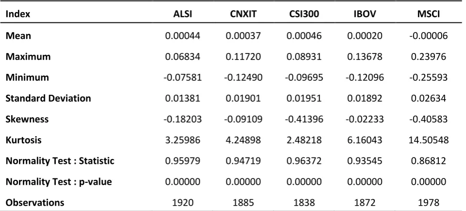
The analysis of data began with various descriptive statistics, as seen in Table 4 below:

Table 4 - Descriptive Statistics per Index

Index ALSI CNXIT CSI300 IBOV MSCI

Mean 0.00044 0.00037 0.00046 0.00020 -0.00006

Maximum 0.06834 0.11720 0.08931 0.13678 0.23976

Minimum -0.07581 -0.12490 -0.09695 -0.12096 -0.25593

Standard Deviation 0.01381 0.01901 0.01951 0.01892 0.02634

Skewness -0.18203 -0.09109 -0.41396 -0.02233 -0.40583

Kurtosis 3.25986 4.24898 2.48218 6.16043 14.50548

Normality Test : Statistic 0.95979 0.94719 0.96372 0.93545 0.86812

Normality Test : p-value 0.00000 0.00000 0.00000 0.00000 0.00000

Observations 1920 1885 1838 1872 1978

From Table 4 above, the mean return for all the indexes are approximately the same with the exception of the MSCI Index having a mean negative return. Analysing the MSCI Index further, the standard deviation is also the largest when compared to the other indexes. Furthermore, the kurtosis, which provides an indicator to how sensitive a variable will be to an infrequent extreme deviation, is also higher than the other indexes. The range between the maximum and minimum, the negative mean return, the standard deviation and the high kurtosis provide the possibility that the MSCI Index tends to be more volatile when compared to the other indexes.

10

skewness statistic, although not equal to zero, is small for all the indexes and skewed towards positive returns.

These indexes will now be analysed individually:

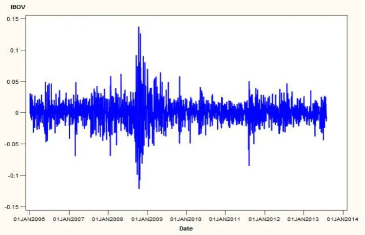
IBOV Sao Paulo Brazil Index (IBOV)

The Ibovespa index is a gross total return index weighted by traded volume and is comprised of

the most liquid stocks traded on the Sao Paulo Stock Exchange (www.bloomberg.com). It is

due to this liquidity that we anticipate a large volatility within the IBOV stock. The volatility of returns for this index is in Figure 1 below:

Figure 1 - Volatility of IBOV Returns

From the figure above, it is evident that there were significant volatility spikes present in Brazil during mid-2008 to early 2009 as well as late 2011. This is evident of the severity of the impact of the Global Financial and Sovereign Debt crisis. It is also visible in the figure above that the volatility persisted and created volatility clusters. In Figure A. 1 in the appendix, the frequency distribution indicates that volatility spikes are present in the tails and that the actual distribution of the IBOV index does not conform to that of a standard Gaussian distribution (red line) but rather a standard student-t distribution, based on a visual interpretation.

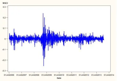
MSCI Russia Index (MSCI)

The MSCI Russia Index is a free-float adjusted market capitalization weighted index that is designed to track the equity market performance of Russian securities listed on the MICEX

Stock Exchange (www.bloomberg.com). The volatility of returns for this index is in Figure 2

11 Figure 2 - Volatility of MSCI Returns

From the figure above, it is evident that large clusters of volatility spikes were experienced in Russia during mid-2008 and early 2009, synonymous with the Global Financial crisis. From the

figure above, the impact of the Sovereign Debt crisis in Greece in 2011 didn’t seem to have too

great an impact on the Russian economy (small volatility spike). In Figure A. 2 in the appendix, the frequency distribution indicates that volatility spikes are present in the tails and that the actual distribution of the MSCI index does not conform to that of a standard Gaussian distribution (red line), based on a visual interpretation. The MSCI index far exceeds the industry benchmark for kurtosis, with significant spikes in the tails of the distribution.

NSE CNXIT Index (CNXIT)

The CNX Nifty, a free float market capitalization index, is the leading index for large companies on the National Stock Exchange of India. It consists of 50 companies representing 24 sectors

of the economy (www.bloomberg.com). The volatility of returns for this index is in Figure 3

below:

12

From the figure above, there were large persistent volatility spikes experienced in India during 2008 persisting into 2009 with a large significant spike occurring in May 2009. What is significant though is the amount of volatility present in the Indian stock market just prior to 2008, perhaps a leading indicator of the Global Financial Crisis. In Figure A. 3 in the appendix, the frequency distribution indicates that volatility spikes are present in the tails of the distribution, while the kurtosis is slightly higher than the benchmark for normality. The skewness for this distribution is also very small, indicating that the asymmetry present is almost negligible.

Shanghai Shenzhen CSI 300 Index (CSI 300)

The CSI 300 Index is a free float-weighted index that consists of 300 A-share stocks listed on

the Shanghai or Shenzhen Stock Exchanges (www.bloomberg.com). The volatility of returns

for this index is in Figure 4 below:

13

From the figure above, there were large persistent volatility spikes experienced in China just prior to 2008 and well into 2009 with the most significant spike occurring in August 2008 (peak of the Global Financial Crisis). It is also evident from the graph above that volatility is persistent as well as clustering, while still remaining mean-reverting. This is attributed to the global presence that China has with respect to the level of exports on a global scale. In Figure A. 4 in the appendix, the frequency distribution indicates that volatility spikes are present in the tails with the kurtosis being lower than the benchmark for normality. A high kurtosis indicates that

the variance results from infrequent extreme deviations, as opposed to frequently “normal”

sized deviations.

JSE All Share Index (ALSI)

The FTSE/JSE Africa All Shares Index is a market capitalization weighted index. Companies included in this index make up the top 99% of the total pre-free float-market capitalization of all

listed companies on the Johannesburg Stock Exchange (www.bloomberg.com). The volatility

14 Figure 5 - Volatility of ALSI Returns

From the figure above, large spikes are evident through 2008 with persistence into much of 2009. It is also noticeable from the graph above that volatility clustering occurs with a relatively constant mean-reversion. In Figure A. 5 in the appendix, the frequency distribution indicates that volatility spikes are present in the tails with the actual distribution only just exceeding the benchmarks for a normal distribution.

In conclusion, from the graphs in this section, it is clear that there is volatility in all the indexes and that this volatility is persistent, clustering and mean-reverting. Other conclusions reached from this section include:

 The frequency distributions of the indexes indicate a deviation from a normal

distribution, in some cases a very slight deviation;

 The skewness statistic is small for all the frequency distributions, indicating that the

leverage effect (bad news impacts the market worse than good news, i.e. asymmetry) is almost negligible;

 The kurtosis for the frequency distributions varies from 2.5 to 6, with an extreme outlier

being the Russian MSCI Index at approximately 14. This indicates that the indexes are moderately affected by infrequent deviations, with the exception of the MSCI Index being more severely impacted.

1.3 Estimation

The univariate time-series of asset returns was estimated using the models specified in the Methodology. The models were fitted to the respective in-sample datasets, and then used to forecast the out-sample dataset observations using a 1-day ahead forecast approach.

ARMA(1,1) - GARCH(1,1) Model

The model estimates for the respective indexes, according to the ARMA (1,1) – GARCH (1,1)

15

Table 5 - Parameter Estimate for ARMA(1,1)-GARCH(1,1)

Parameter Estimates MSCI IBOV CSI300 CNXIT ALSI

7.42E-04 5.93E-04 1.21E-03 1.42E-03 1.58E-03

2.34E-02 -1.25E-02 1.25E-02 3.65E-02 -1.91E-03

1.00E+05 1.00E+00 9.99E-01 9.99E-01 9.99E-01

5.96E-06 5.94E-06 2.48E-06 1.27E-05 1.91E-06

9.19E-02 7.98E-02 4.80E-02 1.62E-01 9.68E-02

9.01E-01 9.01E-01 9.48E-01 8.17E-01 8.96E-01

Following from the table above, the t-statistics for the respective indexes and their corresponding parameters are listed in the table below, all of which were statistically significant at a 90% confidence level:

Table 6 - t-Statistics

t-Statistic MSCI IBOV CSI300 CNXIT ALSI

4.56E-02 1.11E-02 2.40E-04 1.61E-02 2.90E-04

3.00E-02 5.98E-02 5.75E-02 1.24E-02 9.35E-02

< 2e-16 < 2e-16 < 2e-16 < 2e-16 < 2e-16

3.52E-03 2.17E-03 4.84E-02 1.93E-04 7.26E-03

1.21E-09 1.28E-08 1.48E-06 1.26E-08 2.25E-10

< 2e-16 < 2e-16 1.48E-06 1.26E-08 < 2e-16

These estimates were then applied to the out-sample dataset in order to perform the forecasts which will be discussed under the Empirical Results section.

Non-parametric Kernel Regression Model

As mentioned earlier, the model has the benefit that the distribution of the function is not specified which allows the data to keep their original distribution instead of forcing a Gaussian distribution. Similarly to the base model used in this paper, the non-parametric model is fitted to the in-sample dataset and then applied to the out-sample dataset to forecast. The bandwidth of the kernel is a free parameter, i.e. unlike constants or other parameters, a free parameter can be adjusted randomly. The bandwidth exhibits a strong influence on the resulting estimate. Table 7 below provides the bandwidth value for each respective index

based on the cross validation technique described in the methodology:

Table 7 - Bandwidth Estimates

MSCI IBOV CSI300 CNXIT ALSI Bandwidth 0.0003 0.0008 0.0043 0.0007 0.0009

16

Empirical Results

The criteria used to assess the performance of each model’s forecasting ability are the

Predicted Mean Square Error (PMSE), the Diebold-Mariano Test (Diebold and Mariano (1995)), the Mean-Absolute Deviation test and the Variance. This paper makes use of the one-day ahead out-of-sample forecast performance for each model. The four criteria on which the model performance will be assessed, will be discussed in detail:

1.1 Predicted Mean Square Error (PMSE)

The predicted mean square error, calculated from the difference of the actual values from the forecast values generated from the respective models, has the following statistical form:

where and are the actual and predicted values respectively with being the total number

of observations. Intuitively, the smaller this value is; the more accurate the model at predicting asset returns.

1.2 Diebold-Mariano (DM)

The DM test evaluates the significance of the difference between the predicted mean square errors for two models being compared, i.e. this test compares the forecast accuracy of two forecast methods, and is defined as follows:

where is the forecast error obtained for each model, 1 and 2, with referring to a

respective loss function. When many observations are available, the DM test statistic can be adjusted as follows: (Bonga-Bonga and Mwamba (2011))

where and

The Diebold-Mariano test will be performed with three (3) respective hypotheses if no definite conclusion is reached, namely:

The null hypothesis will be that the two models have the same forecasting accuracy. There will

also be two alternatives, namely a “less” and “greater” hypothesis. For the “less” alternative,

the hypothesis will be that model two is less accurate than model 1. For the “greater”

alternative, the hypothesis is the converse of the “less” alternative i.e. that model two is more

accurate than model 1.

1.3 Mean-Absolute Deviation test (MAD)

17

to be irrelevant, taking into account only magnitude instead of direction. The formula to determine this metric is as follows:

where is the total number of forecasts, is the forecast value at the kth _{position and is the}

average of the actual values for the forecast period.

This metric provides an insight into the deviation from the mean of the actual values. Therefore, the smaller the mean-absolute deviation, the more accurate the forecasts will be to the actual values.

1.4 Variance ( )

Is a measure of dispersion of a set of data points from their mean, and is the second moment of any probability distribution. The rationale behind this measure is that, the lower the variance, the lower the dispersion of the data points around the mean. Intuitively, with respect to forecasts, if the variance of the forecasts is closer to the mean of the actual values, then they are more accurate. Variance of the forecasts is defined as the average difference between the squared forecast value and actual value. The formula to determine this metric is as follows:

where is the total number of forecasts, is the forecast value at the kth_{position and is the}

average of the actual values for the forecast period.

As mentioned earlier, the predicted mean square error (PMSE) will provide insight into which model more accurately forecasts the asset return values for each index. The closer the value of the PMSE is to zero, the more accurate it is. Table 8 below provides the PMSE value for each respective index for each of the two models.

Table 8 - PMSE Statistics Comparison

PMSE MSCI IBOV CSI300 CNXIT ALSI ARMA(1,1)-GARCH(1,1) 0.00059 0.00038 0.00074 0.00035 0.00018

NP Kernel Regression 0.00060 0.00006 0.00033 0.00009 0.00006

From the table above, we can conclude that the non-parametric kernel regression technique proves to be more successful at predicting the asset returns for each index with the exception of the MSCI index. Possible solutions to this under prediction could be the bandwidth specification. As mentioned earlier, if the bandwidth is inadequately specified then the model would not be as accurate.

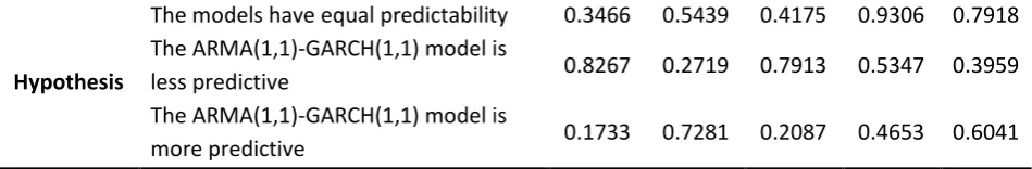
The Diebold-Mariano test compares the forecasting ability of two models, but the interpretation is subjective if a definitive result is not available. Table 9 below provides the p-value statistics for the respective hypotheses for each index.

Table 9 - Diebold-Mariano p-value Comparison

18

Hypothesis

The models have equal predictability 0.3466 0.5439 0.4175 0.9306 0.7918

The ARMA(1,1)-GARCH(1,1) model is

less predictive 0.8267 0.2719 0.7913 0.5347 0.3959

The ARMA(1,1)-GARCH(1,1) model is

more predictive 0.1733 0.7281 0.2087 0.4653 0.6041

From the table above, if we consider the first hypothesis we notice that none of the p-value statistics can be rejected at the 95% confidence level. The first hypothesis is inconclusive surrounding the forecasting ability of the two models, and hence the second hypothesis is considered.

For the MSCI Index, the p-value is high (>50%) indicating that the probability of rejecting the hypothesis that the parametric model (ARMA(1,1)-GARCH(1,1)) is less predictive is only approximately 17.33%. If we then consider the third hypothesis, that the parametric model is more predictive, we observe that the probability of rejecting is 82.67%. No clear conclusion can be drawn from the results for the MSCI Index but the probability that the non-parametric model is more predictive is higher. A similar conclusion is determined for the CSI300 index as well. For the IBOV and ALSI Indexes, the p-value is low (<50%) for the second hypothesis. Following the rationale from the previous indexes above, this indicates that the parametric model has the higher probability of more accurately predicting the out-sample values. The CNXIT index is the only index where the probability that both models forecast with equal accuracy, is high. Therefore, no clear distinction can be made about the forecast accuracy.

The mean-absolute deviation (MAD) measures the spread of the forecasts around the mean of the actual values. Since it uses the absolute value, it is not directional but driven by magnitude, and therefore the smaller of the two values indicates a higher level of accuracy. Table 10 below provides the MAD statistics for the respective models for each index.

Table 10 - Mean-Absolute Deviation (MAD) comparison

MAD MSCI IBOV CSI300 CNXIT ALSI

ARMA(1,1)-GARCH(1,1) 0.0092 0.0019 0.0058 0.0050 0.0035

NP Kernel Regression 0.0075 0.0022 0.0050 0.0066 0.0015

From the table above, the non-parametric model proves to be more accurate at forecasting the out-sample values with the exception of the IBOV and CNXIT indexes which are slightly better forecasted by the parametric model. Due to only three (3) of the five (5) indexes yielding positive results, this method will not be considered as strong evidence in favour of the non-parametric technique.

The variance is a measure of dispersion around the mean. A value of zero for the variance indicates that all values are identical (perfect forecast). Table 11 below provides the variance comparison for the respective models for each index.

Table 11 - Variance Comparison

Variance MSCI IBOV CSI300 CNXIT ALSI ARMA(1,1)-GARCH(1,1) 0.000125 0.000009 0.000036 0.000026 0.000017

NP Kernel Regression 0.000107 0.000006 0.000030 0.000049 0.000003

From the table above, the non-parametric model has the lowest variance for all the indexes with the exception of the CNXIT index.

19

Conclusion

This paper has attempted to compare the out-sample one day ahead forecasting performance of the parametric ARMA(1,1)-GARCH(1,1) model and the non-parametric kernel regression model with the Epanechnikov kernel density. These models were compared using data from January 2006 until July 2013, with the last ten observations being used for the out-sample forecast comparison.

The empirical results provide mixed results in the determination of a more accurate model. Unfortunately, there is no exact methodology to determine which comparative technique is the best at distinguishing between various model forecasts. For this paper however, the PMSE was selected as the primary tool for comparison followed by the Diebold-Mariano test, mean-absolute deviation and then lastly the variance. According to the PMSE, the non-parametric kernel regression technique is more accurate than the parametric model for all the indexes with the exception of the MSCI index. Upon closer analysis, the other three comparative techniques show evidence that the non-parametric model outperforms the parametric base model for the MSCI index. This evidence, combined with the very small difference between the PMSE values, leads to the possible conclusion that the non-parametric technique would yield more consistent results for the MSCI index.

Limitations to the family of non-parametric models are however being discovered, as in Bonga-Bonga and Mwamba (2011) where the forecasting accuracy of the non-parametric models seem to decay as the h-step ahead horizon increases.

20

2

Appendices

Figure A. 1 - IBOV Frequency Distribution

21 Figure A. 3 - CNXIT Frequency Distribution

23

3 References

Bekaert, G., and C. B., Harvey (1995): “Emerging Equity Market Volatility.” NBER Working

Paper Series, Working Paper 5307.

Bollerslev, T. (1987): “A Conditionally Heteroskedastic Time Series Model for Speculative

Prices and Rates of Return.” The Review of Economics and Statistics, Vol. 69, No. 3, pp. 542-547.

Bollerslev, T., Chou, R.C. and Kroner, K.F. (1992): “ARCH Modeling in Finance: A Review of

Theory and Empirical Evidence.” Journal of Econometrics, Vol. 52, pp. 5-59

Bonga-Bonga, L and Mwamba, M (2011): “The predictability of stock market returns in South

Africa: Parametric vs. Non-parametric methods.” South African Journal of Economics, Vol. 79, No. 3, pp. 301-311.

Diebold, F.X. and Mariano, R.S. (1995): “Comparing Predictive Accuracy.” Journal of Business

and Economic Statistics, Vol. 13, pp. 253-63.

Fama, E. F (1965): “The behavior of Stock Market Prices.” The Journal of Business, Vol.38, No.

1, pp.34 – 105.

Fama, E. F and Schwert, G. W (1977): “Asset Returns and Inflation.” Journal of Financial

Economics, Vol. 5, pp. 115-146.

Granger, C. W. J. and Morgenstern, O. (1970): “Predictability of Stock Market Prices.” Studies

in Business, Industry and Technology, Heath Lexington Books.

Harvey, C. R (1995): “Predictable Risk and Returns in Emerging Markets.” National Bureau of

Economic Research (NBER), Working Paper No. 4621.

Jefferis, K. and Thupayagale, P. (2008): “Long Memory in Southern African stock markets.”

South African Journal of Economics, 76(3): pg. 384-398.

Lo, A. and Mackinlay, C. (1999): “A Non-Random Walk Down Wall Street.” Princeton University

Press, Princeton.

Mandelbrot, B (1963): “The Variation of Certain Speculative Prices.” Journal of Business, Vol.

36, pp. 394-419.

Mwamba, J. M. (2011): “Modelling Stock Price Behaviour: The Kernel Approach.” Journal of

Economics and International Finance,Vol. 3(7), pp. 418-423.

Nadaraya, W. (1964): “On Estimating Regression.” Probability Theory and its Applications, Vol.

10, pp. 186-190.

Pesaran, M. H and Timmermann, A. (1995): “Predictability of Stock Returns: Robustness and

economic significance.” The Journal of Finance, Vol. 50, No. 4, pp. 1201-1228.

Watson, G.S. (1964): “Smooth Regression Analysis.” Sankhyā Ser. A, 26, pp. 359-378

Wurgler, J. (1999): “Financial Markets and the Allocation of Capital.” Journal of Financial