Munich Personal RePEc Archive
An effective replicator equation for
games with a continuous strategy set
Ruijgrok, Matthijs and Ruijgrok, Theo
Utrecht University, Utrecht University
13 December 2013
Online at
https://mpra.ub.uni-muenchen.de/52198/
(will be inserted by the editor)
An effective replicator equation for games with a continuous
strategy set
M. Ruijgrok · Th. W. Ruijgrok
Received: date / Accepted: date
Abstract The replicator equation for a two person symmetric game, which has an interval of the real line as strategy space, is extended with a mutation term. Assuming that the distribution of the strategies has a continuous density, a partial differential equation for this density is derived. The equation is analysed for two examples. A connection is made with Adaptive Dynamics.
Keywords Evolutionary games· Replicator equation · Mutation· Dynamic stability·Partial differential equations
Mathematics Subject Classification (2000) MSC 91A22
1 Introduction
The use of continuous strategy sets in replicator dynamics introduces two new prob-lems, compared to the situation where the set of strategies is finite. First, there are dif-ferent notions of ’nearness’ possible, associated with the strong and the weak topol-ogy, respectively. The salient difference between these topologies is illustrated by the following property. LetSbe the set of strategies and letδxwithx∈Sdenote the Dirac
distribution concentrated on{x}. In the strong topology, the distance betweenδxand
δy is equal to 2, ifx6=y. In the weak topology, the distance betweenδx andδy is
small, if|x−y|is small. The choice of a particular topology has implications for the concept of evolutionary stability.
The other problem is that it has not been possible to actually solve the replicator equation in the case of continuous strategy sets, except for the case thatS=Rand M. Ruijgrok
Mathematical Institute, Utrecht University, Budapestlaan 4, 3584 CD Utrecht, The Netherlands Tel.: +31-30-2531525
E-mail: [email protected]
Th. W. Ruijgrok
the assumption that the initial distribution is Gaussian. It was shown in Oechssler and Riedel (2002) that the distribution then retains this shape during the evolution in time and the replicator equation reduces to a coupled set of ordinary differential equations for the mean and the variance of the distribution.
The impossibility of solving the replicator equation for more general initial distribu-tions makes it difficult to establish dynamical stability criteria for equilibrium strate-gies of the underlying game. In the case of a finite set of stratestrate-gies, we have the concept of an Evolutionary Stable Strategy (ESS) of a game. ESS is a static con-cept, computable from the knowledge of the payoff function, but it is tied to dynamic stability through the theorem that an ESS of a symmetric game is an asymptotically Lyapunov stable equilibrium of the corresponding replicator equation. The definition of an ESS can be generalized to games with a continuous strategy set, but it has been shown that the ESS condition is no longer sufficient for a strategy to be a Lyapunov stable solution of the replicator equation. Various stronger static stability concepts have been introduced, which have fairly complicated interrelations, see Oechssler and Riedel (2002) and Cressman (2005).
In this paper we derive a version of the replicator equation which has the property that it can be analysed fairly deeply and can easily be solved numerically. In particular, we can find exact expressions in the limit that time goes to infinity, in the case of two important examples.
The equation we start with is the replicator equation with a mutation-term, which was introduced in Bomze and B¨urger (1996). We then restrict the allowed distributions to those which have a (twice continuously differentiable) density function with full sup-port onS. The natural topology in this case is the strong topology, which implies that the space of densities we will be working with is a subset ofL1(S). We then make some, not too demanding, assumptions on the mutation kernel and apply an approxi-mation method which is familiar from statistical physics. This then leads to a partial differential equation with boundary conditions for the density of the distribution. The equation is nonlinear and has non-local terms, .
This equation clearly does not allow for singular distributions such asδxas a solution,
so we will not be able to make stability statements directly aboutδx. However, we
will quite often find that solutions converge to a Gaussian centered at somex∈Sand with width going to zero as the size of the mutation term goes to zero.
The equation is analyzed in two cases. The first one corresponds toS=Rand the payoff function
f(x,y) =−x2+2axy,
witha∈R. In section 3 we will show that for any initial condition, the solution will converge to a Gaussian with widthε, whereε2is the size of the mutation term. The
meanmof this Gaussian converges tom=0 if and only ifa<1. Ifa>1 thenm
diverges to infinity.
In the second example,S=Rand
We will show in Section 4 that, also in this case, all initial distributions eventually tend to a Gaussian shape. However, the mean of this Gaussian always converges to
m=0, but now it is the width of the distribution that shows interesting dynamics. Depending on the initial condition, this width will either converge toεor diverge to infinity.
In section 5 we conclude with some remarks about the connection between the results derived in these examples and local stability criteria. Also, we will consider how this version of the replicator equation relates to Adaptive Dynamics.
2 Derivation of the equation
The two-player game under consideration is symmetric and is defined through the payoff function f(x,y). The domain of this function isS×S, whereS⊂Ris a closed interval. We allowS=R.
LetBbe the Borelσ-algebra onSand∆(S)be the subset of probability measures
of the measure space(S,B). The state of the game at timet is defined by the
dis-tribution of the strategies in the population, given by P(t)∈∆(S). IfA∈B, then
P(t)(A) =
Z A
P(t)(dx)is the fraction of players in the population who play a strategy
x∈Aat timet.
There are two factors driving the evolution ofP(t): selection and mutation. The selec-tion terms describes the standard assumpselec-tion of replicator dynamics, namely that the fraction of strategies that have a higher payoff compared to the average payoff will increase in the population, at the expense of strategies that do worse than average. Assume the distribution of strategies is given byP∈∆(S). The expected payoff of a strategyQ∈∆(S)against this population is defined as:
π(Q,P) =
Z S
Z S
f(x,y)Q(dx)P(dy). (1) In particular, the expected payoff of a pure strategyx∈Sagainst the population dis-tributionPis given by
π(x,P)≡π(δx,P) = Z
S Z
S
f(x,y)δx(dx)P(dy) = Z
S
f(x,y)P(dy). (2) We define the average payoff of the distributionP∈∆(S)as
π(P) =π(P,P). (3)
The relative fitness of strategyx∈S, against the population distributionPis defined as:
φ(x,P) =π(x,P)−π(P). (4)
Agents sometimes spontaneously change their strategy, by mistake or as a type of
time interval is the same for all agents. Let µ>0 and µdtbe the probability that an agent using strategyx∈Smutates during a short time intervaldt. Letm(y,x)be the probability distribution of this mutated strategy, i.e. ifA∈Bthen the probability that
strategyxmutates to a strategy inAis
Z A
m(y,x)λ(dy), withλ the Lebesgue-measure onS.
An important assumption in the following is thatm(y,x)>0 for all(x,y)∈S×S. This implies that all strategies have a positive probability to arise from a mutation, and in fact every strategy will be present in the population for allt>0.
For a given distributionP(t)of the strategies at timet, andA∈B, the change per
unit time of the fraction of strategies inA, due to mutations, is given by:
µ
Z A
Z S
m(y,x)P(t)(dx)λ(dy)−
Z A
Z S
m(x,y)λ(dx)P(t)(dy)
. (5)
Combining (4) and (5), and suppressing in the notation the t-dependence of P(t), leads to the mutation-selection equation introduced by B¨urger and Bomze (1996):
d
dtP(A) =
Z A
φ(x,P)P(dx) +µ
Z A
Z S
m(y,x)P(dx)λ(dy)−
Z A
Z S
m(x,y)λ(dx)P(dy)
.
(6)
The differential equation (6) is defined on the Banach-spaceM = (M(S,B),||.||1).
Here,M(S,B)is the vectorspace of all signed measures on(S,B)and||.||1is the
variational norm onM(S,B)given by:
||Q||1=sup
f∈F| Z
S
f(x)Q(dx)|.
The supremum is taken over the setF of all measurable functions f :S→Rwith supx∈S|f(x)| ≤1.
The variational norm induces the strong topology. In this topology||δx−δy||=2 if
x6=y, so even though the strategiesxandycan be very close, the corresponding monomorphic distributions are not. An alternative measure of closeness is the Pro-horov metric, which induces the weak topology and is used in Oechssler and Riedel (2002) and Cressman and Hofbauer (2005).
Some important properties ofM, equation (6) and its solutionP(t)are:
– For probability measures with a continuous density w.r.t. the Lebesgue mea-sure, the variational norm is equivalent to theL1norm (see Oechssler and Riedel
(2001)). This means that two of these measures are close in the variational norm if and only if their densities are close in theL1norm.
– If the payoff function f(x,y)is bounded, then equation (6) has a unique solution, defined for allt>0. (see B¨urger and Bomze (1996))
2.1 Assumption and approximation
Assume that the measurePhas a density w.r.t the Lebesgue measure for allt≥0. We write:
P(t)(dx) =ρ(x,t)dx.
We will, moreover, assume thatρ(x,t)is twice continuously differentiable with re-spect tox. Using the fact that
π(x,P) =
Z S
f(x,y)ρ(y,t)dy
the equation (6) now reduces to:
∂
∂tρ(x,t) =
Z S
f(x,y)ρ(y,t)dy−
Z S
Z S
f(x,y)ρ(y,t)ρ(x,t)dy dx
ρ(x,t) +
µ
Z S
m(x,y)ρ(y,t)dy−ρ(x,t)
Z S
m(y,x)dy
. (7)
To simplify (7) further, we will use an approximation that is standard in deriving the Fokker-Planck equation from the master equation in statistical physics (see van Kam-pen (1975)), and was already used by Kimura (1965) in a context similar to ours. For the moment we will take S=R. The probability distribution of the strategies y∈S that arise as a mutation from a strategyx∈S is assumed to be of the form
m(y,x) =m˜(|y−x|,x). The distribution ˜m(z,x)is symmetric inz, is rapidly decreas-ing asz→ ±∞and has variation
Z ∞
−∞
z2m˜i(z,x)dz=σ2(x). The higher order moments
of ˜m(z,x)are at least ofO(σ4(x)). A typical form for the mutation kernel is the
Gaus-sian:
m(y,x) =√ 1
2πσ(x)e
−(x−y)2/2σ2(x)
,
whereσ(x)is small. We can then write:
Z ∞
∞
m(y,x)ρ(y,t)dy=
Z ∞
∞ ˜
m(y−x,x)ρ(y,t)dy=
Z ∞
∞ ˜
m(z,x)ρ(z+x,t)dz
=
Z ∞
∞ m˜(z,x) (ρ(x,t) +
∂
∂xρ(x,t)z+
1 2
∂2
∂x2ρ(x,t)z
2+. . .)dz
=ρ(x,t) +1
2σ
2(x)∂2
∂x2ρ(x,t) +O(σ
4(x)) (8)
Substituting (8) in (7) and neglecting the higher order terms, we find the equation that is referred to in the title of this paper:
∂
∂tρ(x,t) =
Z S
f(x,y)ρ(y,t)dy−
Z S
Z S
f(x,y)ρ(y,t)ρ(x,t)dy dx
ρ(x,t) +
1 2µσ
2(x)∂2
In the case thatSis a finite interval, the mutation term near the boundaries ofSneeds to be adapted, so that no mutations outsideSare possible. This is a technically cum-bersome operation, which can be solved by keeping the equation (9), but supplying it with reflecting, or Neumann, boundary conditions:
∂
∂xρ(x,t)|∂S=0. (10)
2.2 Existence and properties of the solution
The equation (9) is a nonlinear, non-local, reaction diffusion equation. The function space we will be working on is that of twice continuously differentiable densities
ρ(x), such thatρ,ρxandρxxare all inL1(S)and satisfying the Neumann boundary
conditions (10).
From (9) and (10), we recover the important property that if
Z Sρ(
x,0)dx=1, then
Z S
ρ(x,t)dx=1 (11)
for allt>0, as is easily checked.
It follows from standard positivity results for parabolic equations that if the initial valueρ0(x)>0 for allx∈S, thenρ(x,t)>0 for allt≥0. We will from now on always assume that ρ(x,t)>0, for all x∈S andt ≥0. Thus, the support of the measurePcorresponding toρis the full strategy setS.
IfSis compact, then existence ofρ(x,t)in the above mentioned function space can be proved for allt≥0. This follows from the fact that if f(x,y)is bounded onS×S, the reaction term is clearly continuous inρand bounded:
|
Z S
f(x,y)ρ(y,t)dy−
Z S
Z S
f(x,y)ρ(y,t)ρ(x,t)dy dx| ≤
Z S|
f(x,y)|ρ(y,t)dy+
Z S
Z S|
f(x,y)|ρ(y,t)ρ(x,t)dy dx≤
max(x,y)∈S×S|f(x,y)|
Z S
ρ(y,t)dy+
Z S
Z S
ρ(y,t)ρ(x,t)dy dx
=2 max(x,y)∈S×S(|f(x,y)|),
where we have used (11) and the positivity ofρ. Comparison theorems for parabolic equations (Pao (1992)) complete the proof.
In the case thatS=R, a solution can not be guaranteed for all time, as follows from the following example adapted from Cressman and Hofbauer (2005). Let f(x,y) =x2
and12µσ2(x) =ε2be constant. Then equation (9) becomes: ∂
∂tρ(x) =
x2−
Z
R
x2ρ(x,t)dx
ρ(x,t) +ε2∂2 ∂x2ρ(x).
It can be checked thatρ(x,t) =√ 1 2πV(t)e
−(x−2Vm((tt)))2 is a solution of the above equation,
ifV(t)andm(t)satisfy the diferential equations:
The solutionV(t)will ”blow up” in finite time, for every initial valueV(0). Note that the correspondingρ(x,t)will ”flatten out” in that time.
In the examples considered below,S=R. However, existence of solutions for all times will be shown by construction.
3 Application to a quadratic payoff function
We will takeS=Rand consider the payoff function f(x,y) =−x2+2axy,
witha∈R. The symmetric game corresponding to this payoff function has, for all a∈R, a unique, strict, Nash equilibrium in pure strategies, namelyx=0.
Using the fact that
Z S
ρ(x,t)dx=1, we find that
Z S
f(x,y)ρ(y,t)dy−
Z S
Z S
f(x,y)ρ(y,t)ρ(x,t)dy dx=−x2+2axx(t)+x2(t)−2ax2(t),
with
xn(t) = Z ∞
−∞
xnρ(x,t)dx.
The dependence ofxnontwill often be suppressed in the notation. We will assume
thatµσ2(x) =ε2is independent ofxand small. Equation (9) then becomes: ρt=
−x2+2axx+x2−2ax2ρ+ε2ρ
xx. (12)
In addition to this equation, we have an initial condition
ρ(x,0) =ρ0(x), (13)
such thatρ0(x)>0,
Z S
ρ0(x)dx=1 andρ0(x)twice continuously differentiable on R. As shown in the previous section, these conditions imply that
Z S
ρ(x,t)dx=1,
ρ(x,t)>0 and ρ(x,t)twice continuously differentiable for allt >0. This in turn implies thatρ(x,t)∈L1(R)andρ(x,t)∈L2(R).
3.1 The Wei-Norman method
Although equation (12) is nonlinear and contains non-local terms, it can be solved explicitly. This is done by exploiting its linear appearance. We first assume thatxand
x2are given functions oft. Equation (12) then becomes a linear equation with
methods have been devised, notably the Wei-Norman method. Using this method, equation (12) is solved yielding the solution
ρ(x,t;x,x2). (14)
Solving the two equations
x(t) =
Z ∞
−∞xρ(x,t;x,x
2)dx , x2(t) =
Z ∞
−∞x
2ρ(x,t
;x,x2)dx
for(x,x2)gives a unique solution, which can be substituted in (14) to give the
solu-tion of (12). In fact, we will only need the equasolu-tion forx.
We recall some facts about Lie algebras, which play a role in the Wei-Norman method. A finite, real Lie algebra L is a vector space over the reals, spanned by a finite
number of elements{X1, . . . ,Xn}. This vector space is equipped with a Lie bracket
[, ]:L×L →L. This bracket is bi-linear, and satisfies[X,X] =0, for allX∈L
and Jacobi’s identity[X,[Y,Z]] + [Z,[X,Y]] + [Y,[Z,X]] =0, for allX,Y,Z∈L.
In our case, the elements ofL are linear operators onL2(R)and the bracket is
de-fined as[X,Y] =XY−Y X.
Define[L,L] ={[X,Y]|X,Y∈L}. A Lie algebraL is calledsolvableif the series L,[L,L],[[L,L],[L,L]], . . .eventually terminates in 0.
Theorem 1 LetL be a finite, solvable, real Lie algebra, generated by{X1, . . . ,Xn}.
The solution to the initial value problem
dU dt =
n
∑
i=1 ai(t)Xi
!
U , U(0) =U0
can be written in the form
U(t) =exp(g1(t)X1)exp(g2(t)X2). . .exp(gn(t)Xn)U0.
Moreover, the functions gi(t)can be found as solutions of ordinary differential
equa-tions involving the coefficients ai(t).
Proof See Wei and Norman (1964).
To apply this theorem to (12), we first introduce the scalings x=εξ,t=ετ and
ρ(x,t) = (1
ε)ρˆ(x/ε,t/ε), and find x(t) =
Z ∞
∞
xρ(x,t)dx= (1/ε)
Z ∞
∞
xρˆ(x/ε,t/ε)dx=ε
Z ∞
∞
ξρˆ(ξ,τ)dξ=εξ(τ),
and similarly
x2(t) =ε2ξ(τ), Z ∞
∞
ˆ
Substituting, equation (12) becomes independent ofε:
ˆ
ρτ=−ξ2+2aξ ξ+ξ2−2aξ2ρˆ+ρˆ
ξ ξ. (15)
We can write equation (15) in the form
ˆ
ρτ=Z+0.Y+2aξX+ (ξ2−2aξ2−1)Iρˆ, (16)
where for f∈L2(R):
Z f =
d2 dξ2−ξ
2+1
f
Y f= d
dξ f X f=ξ f
I f=f.
The elements of{X,Y,Z,I} are the generators of a Lie algebra with the following commutation relations:
[Z,X] =2Y , [Z,Y] =2X , [Y,X] =I, (17) and[A,I] =0 for allA∈ {X,Y,Z,I}.
It is easy to check that this Lie-algebra is solvable, so that the theorem can be applied. We write the solution of the initial value problem (15) in the form:
ˆ
ρ(ξ,τ) =egI(τ)IegX(τ)XegY(τ)YegZ(τ)Zρ0ˆ (ξ), (18)
where
ˆ
ρ0(ξ) =ερ0(εξ),
the rescaled initial value. The order of the operators could have been chosen differ-ently, but the sequel will show that the form (18) is very practical.
To derive the differential equations for the functionsgi(τ), we will repeatedly use the
formula:
eλABe−λA=B+λ[A,B] +λ
2
2![A,[A,B]] +
λ3
3![A,[A,[A,B]]] +. . . , (19) whereAandBare elements of a Lie-algebra andλ ∈C. As a special case we note that:
eλAA=AeλA,
terminates, which makes it possible to write for anyA,B∈ {Z,Y,X,I}:
eλAB=L(Z,Y,X,I)eλA,
whereL(Z,Y,X,I)is some linear expression in its arguments. Differentiating (18) with respect toτyields:
ˆ
ρτ= g′II egIIegXXegYYegZZ+g′
XegIIX egXXegYYegZZ+g′YegIIegXXY egYYegZZ
+g′ZegIIegXXegYYZ egZZρˆ
0(ξ), (20)
whereg′i= d
dτgi(τ).
Using (19) and the commutation relations, we find:
egXXY= (Y−g
XI)egXX
egYYZ= Z−2g
YX−g2YI
egYY
egXXZ= Z−2g
XY+g2XI
egXX.
Substituting these expressions in (20) and collecting the coefficients, we find:
ˆ
ρτ= g′II+g′XX+gY′(Y−gXI) +gZ′(Z−2gXY+g2XI−2gYX−g2yI)
ˆ
ρ
= g′ZZ+ (gY′ −2gXg′Z)Y+ (g′X−2gYg′Z)X+ (g′I−g′YgX+ (g2X−g2Y)g′Z)I
ˆ
ρ.
(21)
Comparing (21) with (16) yields the system of equations:
g′Z=1
g′Y−2gXg′Z=0
g′X−2gYg′Z=2aξ
g′I−g′YgX+ (g2X−gY2)g′Z=ξ2−2aξ
2
−1, (22)
with intial conditionsgI(0) =gX(0) =gY(0) =gZ(0) =0. We will ignore the last
equation, since in the expression
ˆ
ρ=egIIegXXegYYegZZρ0ˆ (ξ)
the factoregIIis simply a normalization term, which can also be calculated from the
conditionR
Rρˆ(ξ,t)dξ=1.
The other three equations can be easily integrated and we find in particular that
gZ(τ) =τ.
ForgX(τ)andgY(τ)we can find explicit expressions which involveξ, however their
3.2 Solution for large values ofτ
Consider first the result of the operatoregZ(τ)Zacting on an initial function ˆρ0(ξ). Let esZρ0ˆ (ξ) =f(ξ,s),
(withs∈R) then f(ξ,s)is the solution of the partial differential equation
∂f
∂s =Z f = (−ξ 2+
1)f+∂
2f
∂ ξ2 , f(ξ,0) =ρ0ˆ (ξ). (23)
It is well known that the eigenfunctions ofZ are the Hermite functions {φn(ξ)},
n=0,1, . . ., with corresponding eigenvaluesλn=−2n. The Hermite functions form
an orthonormal base ofL2(R), with
φ0(ξ) = (2π)−1/4e−ξ2/2
Since ˆρ0(ξ)∈L2(R), we can write
ˆ
ρ0(ξ) =
n=∞
∑
n=0
anφn(ξ) , an= Z
R
φn(ξ)ρ0ˆ (ξ)dξ.
We note thata0>0, becauseφ0(ξ)ρ0ˆ (ξ)>0. The solution of (23) can now be written
as:
esZρ0ˆ (ξ) = f(ξ,s) =
n=∞
∑
n=0
e−2n sanφn(ξ). (24)
From this expression, it follows that:
lim
s→∞||e
sZρˆ
0(ξ)−a0φ0(ξ)||2=0.
In other words, whatever the initial distribution ˆρ0(ξ), the expressionesZρ0ˆ (ξ)ass
goes to infinity, will tend to a normal distribution (multiplied by a positive factor), with mean equal to zero and variance equal to one.
The action of the operatoresYon functionsg∈L2(R)is that of the shift operator: esYg(ξ) =esdxdg
(x) =g(ξ+s),
for alls∈R.
Finally,esX acts as a simple multiplication:
esXg(ξ) =esξg(ξ).
We are now in a position to write down, for every givenξ(τ)and initial function ˆ
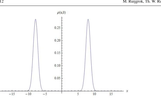
Fig. 1 Initial condition for equation (15) is a sum of Gaussians, both with varianceσ2=0.49, centered at
x=−7.9 andx=8.0.
equation
ξ(τ) =
Z
R
ξρˆ(ξ,τ;ξ)dξ,
which would give a complete solution of the initial problem (12). Deriving an explicit expression forξfor a general initial distribution ˆρ0(ξ)is, however, not possible. This is not a major problem, as the early development of the distribution is less interesting and can, for a specific initial distribution, be found numerically. What is much more important is the eventual fate of the solution. As it happens, the asymptotic behaviour of the solution for largeτcan be found, and it is independent of the initial distribution.
We approximate ˆρ(ξ,τ)for largeτas follows: ˆ
ρ(ξ,τ) =egI(τ)IegX(τ)XegY(τ)YegZ(τ)Zρ0ˆ (ξ)
=n(τ)egX(τ)XegY(τ)YeτZρ0ˆ (ξ)
≈n(τ)egX(τ)XegY(τ)Ye−ξ2/2
=n(τ)egX(τ)ξe−(ξ+gY(τ))2/2=n(τ)e−(ξ−gX(τ)+gY(τ))2/2, (25)
wheren(τ)is the aforementioned normalisation factor, which, with some abuse of notation, has absorbed allτ-dependent terms in each step of the derivation.
This approximation is a Gaussian, with variance=1 and meanx=gX(τ)−gY(τ)).
Using (22), we then have
dx
dτ =g′X(τ)−gY′(τ) =−2(gX(τ)−gY(τ)) +2ax(τ) = (−2+2a)x, (26)
with solution
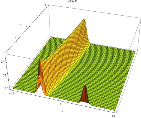
[image:13.595.73.388.69.261.2]Fig. 2 Short-time evolution of initial condition of Figure 1.a=0.9.
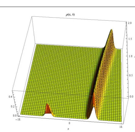
Fig. 3 Long-time evolution of initial condition of Figure 1.a=0.9.
From this expression we see that, asymptotically for τ→∞, the solution of (12) shows one of two possible behaviours. Ifa<1, the solution converges to a Gaussian with width equal to one, and a mean that converges exponentially to zero. Ifa>1, the solution still converges to a Gaussian with width one, but now the mean grows unboundedly.
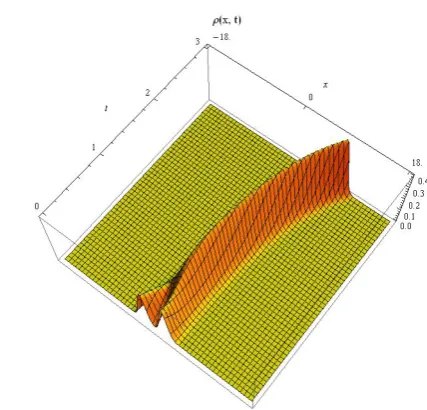
[image:14.595.76.324.88.282.2] [image:14.595.84.314.322.515.2]Fig. 4 Long-time evolution of initial condition of Figure 1.a=1.1.
Fig. 5 Initial condition for equation (15) is a sum of Gaussians, both with varianceσ2=0.49, centered at
x=−1.9 andx=2.0.
normal distribution centered atx=0 and a width ofε, for all initial distributions. This convergence happens on a time scale of 1/ε. Fora>1 the distribution does not converge.
3.3 Numerical simulations
The figures 1 through 6 were made by discretizing the x-variable on the interval
[image:15.595.80.303.69.287.2] [image:15.595.76.329.315.488.2]Fig. 6 Long-time evolution of initial condition of Figure 5.a=1.5.
(9), the second derivative was replaced by the standard approximation and integration by a simple summation. The resulting system of ordinary differential equations for
xi(t)was then solved, using Mathematica routines. Although this is a very
unsophis-ticated method, the results agree completely with the analysis of the previous section. In the Figures 1 and 2 we have takena=0.9 and as initial condition a sum of two sharp peaks, with equal mass and width and almost symmetrically placed. In Figure 2, the evolution is shown on a short time-scale. Initially, the two peaks co-exist until at aboutt=0.05 the peak atx=8 collapses and all the mass of the distribution be-comes concentrated near the peak atx=−7.9. On this time scale, the location of the peaks has hardly moved. In Figure 3 the further evolution is shown. After the collapse of the right peak, the now single-peaked distribution takes on a Gaussian shape and the mean of this distribution moves towardsx=0. Convergence to the steady state, approximated by (25) is virtually complete at aboutt=15.
In Figure 4 we have taken the same initial condition as in Figure 1, but now with
a=1.1. We see that it is now the left peak which collapses after a short period. The surviving peak at the right again assumes a Gaussian shape and starts to move to-wards infinity, as predicted by equation (26).
Figure 5 shows an initial condition which is again the sum of two peaks, but now close together. Figure 6 shows that these peaks first merge to one peak, centered at approximatelyx=0, then this peak starts to move away from this position, because
[image:16.595.81.295.83.288.2]4 Payoff function with fourth order term
We now apply the method of the previous section to the payoff function
f(x,y) =−x2+x2y2,
and the strategy setS=R. Substituting this function in (9) and using the scalings x=εξ,t=ετandρ(x,t) = (1
ε)ρˆ(x/ε,t/ε), we find
ˆ
ρτ=−ξ2(1−ε2ξ2) +ξ2(1−ε2ξ2)ρˆ+ρˆ
ξ ξ. (27)
We can write equation (27) in the form
ˆ
ρτ=Z+0.V+ε2ξ2W+ (ξ2−ε2ξ22−1)Iρˆ, (28)
where for f∈L2(R):
Z f =
d2 dξ2−ξ
2+
1
f
V f =ξ d dξ f
W f=ξ2f I f =f.
The operatorVwas chosen to make{Z,V,W,I}a closed Lie-algebra. The commuta-tion relacommuta-tions are:
[Z,W] =4V+2I , [Z,V] =2Z+4W−2I , [W,V] =−2W, (29) and[A,I] =0 for allA∈ {X,Y,Z,I}.
This Lie-algebra is not solvable, and the series on the rightside of (19) does not ter-minate for all elements of the algebra. However, it is still possible to sum the series, as we shall show later. Because of this, we believe that the conclusion of the theorem of Wei and Norman still holds, although the condition of solvability is not met. Assume therefore that the solution of (28) has the form
ˆ
ρ(ξ,τ) =egI(τ)IegV(τ)VegW(τ)WegZ(τ)Zρˆ
0(ξ). (30)
To find the equations forgV,gW andgZ, we differentiate (30) with respect toτ:
ˆ
ρτ= g′II egIIegVVegWWegZZ+g′
VegIIV egVVegWWegZZ+gW′ egIIegVVW egWWegZZ
+g′ZegIIegVVegWWZ egZZ
ˆ
ρ0(ξ). (31)
It is fairly straightforward to derive that:
egVVW =e2gVWegVV egWWZ= Z−g
W(2I+4V) +4g2WW
Define[V,Z](n)= [V,[V,Z](n−1)]forn≥1 and[V,Z](0)=Z. Then
egVVZe−gVV=
∞
∑
n=0 gVn
n (32)
After calculation of a few iterations, it becomes clear that:
[V,Z](n)=an[V,Z] +bnW, a1=1,b1=0 (33)
Using the commutation rules we find the recursions:
an=−2an−1 bn=2bn−1−2(−2)n,
with solutions:
an= (−2)(n−1),bn=−(2n+ (−2)n) (34)
Substituting (34) and (33) in (32) leads, after some manipulation, to
egVVZ= (e−2gVZ−2 sinh(2g
V)W−e−2gVI)egVV
We can now calculate:
egVVegWWZ egZZ=egVV(Z−g
W(2I+4V) +4gW2W)egWWegZZ=
(e−2gVZ−2 sinh(2g
V)W−e−2gVI−2gWI−4gWV+4g2We2gVW)egVVegWWegZZ
After substitution and collecting terms, we find that
ˆ
ρτ= (g′I−2g′ZgW)I+ (gV′ −4g′ZgW)V+
(gW′ e2gV+g′
Z(−2 sinh(2gV) +4gW2e2gV))W+g′Ze−2gVZ)
ˆ
ρ. (35)
Comparing the terms of (31) and (35), we find the set of differential equations
e−2gVg′
Z=1
gV′ −4gWg′Z=0
e2gVg′
W+ (−2 sinh(2gV) +4gW2e2gV)g′Z=ε2ξ2. (36)
As in the previous section, we ignore the equation forgI.
The equation forgZcannot be solved directly. However, if we assume thatgV(τ)>
α for someα∈Rand for allτ>0, thene2gV(τ)>eα>0 and thereforeg
Z(τ) = Rτ
0e2gV(τ
′)
dτ′ is an increasing function such that limτ→∞gZ(τ) =∞. We will show
4.1 Solution for largeτ
From (24) it follows that
lim
τ→∞e
gZ(τ)Zρ0ˆ (ξ,τ) = lim τ→∞
n=∞
∑
n=0
e−2n gZ(τ)a
nφn(ξ) =a0φ0(ξ),
where convergence is in theL2norm. We will take this multiple of a Gaussian of variance one and mean zero as the approximation ofegZ(τ)Zρ0ˆ (ξ,τ)for largeτ.
The operatorV is the generator of scalings, as follows from the fact thateλVf(x):=
g(x,λ)is the solution of
∂
∂ λg(x,λ) =V g(x,λ) =x ∂
∂xg(x,λ), g(x,0) =f(x)
It is easily checked thatg(x,λ) =f(eλx)is the solution of the above equation. There-fore,egVVφ0(ξ) =φ0(egVξ), a Gaussian with mean zero, but width now stretched by
a factoregV.
Finally,egWW is simply a multiplication byegWξ2.
Combining these elements we have that for largeτ, an approximation is given by
ˆ
ρ(ξ,τ) =n(τ)egV(τ)VegW(τ)WegZ(τ)Zρ0ˆ (ξ)≈n(τ)egV(τ)Ve(gW−12)ξ2
=n(τ)e−12(1−2gW)e2gVξ2.
In other words, for every initial condition, the solution converges to a Gaussian with mean equal to zero, but with variance
σ2= (1
−2gW)−1e−2gV (37)
This approximation closes the set of differential equations (36), since for largeτwe know thatξ2can be approximated by σ2. This then yields an autonomous set of
ordinary differential equations, which should be studied for large values ofτ. However, we are mainly interested in the evolution ofσ2, for which it is possible to
derive a simple equation. For this,σ2is substituted forξ2in (36), yielding:
e2gVg′
W =ε2σ2−1+ (1−4gW2)e4gV.
Then:
d
dτσ= (1−2gW)− 3/2g′
We−gV −(1−2gW)−1/2e−gVgV′ =σ((1−2gW)−1g′w−gV′)
=σ(σ2e2gVg′
W−gV′) =σ(σ2(ε2σ2−1+ (1−4g2W)e4gV)−4gWe2gV)
=σ(σ2(ε2σ2−1+2σ−2e2gV−σ−4)−2(e2gV−σ−2))
=ε2σ5
−σ3
−σ−1+2σ−1=ε2σ5
−σ3+σ−1.
Or, in terms ofσ2:
1 2
d dτσ
2=ε2(σ2)3
This equation has two fixed points, which for smallεhave the form:
σ2
a=1+
1 2ε
2+O(ε4) σ2
r =
1
ε2+O(1)
The fixed pointσ2
Ais an attractor for equation (38) which attracts all solutions with
0<σ2(0)<σ2
r, whileσR2is a repellor and all solutions withσ2(0)>σr2diverge to
infinity.
Additional evidence for the correctness of the above analysis comes from the fact that
ˆ
ρ(ξ,t) =√ 1
2πα(t)e
−2αξ22(t),
is a solution of (27) and the equation forα2is exactly equal to the equation (38), with σ2replaced byα2.
In terms of the original variablesxandt, all solutions of the unscaled equation for
ρ(x,t)converge to a Gaussian shape with mean zero. The variance either converges to a fixed point ofO(ε2), or it diverges to infinity. We will denote the distribution
corresponding toσ2
a as ρ(x). The equation has another stationary solution, namely
a Gaussian with mean zero and variance close to one, which corresponds withσ2
r.
This stationary solution is unstable, since any Gaussian with mean zero and variance slightly different fromσ2
r will not remain close to this solution.
It would be tempting from the above to conclude thatρ(x)is a stable solution of (27). This is, however, not the case, as follows from the following counterexample which is adapted from Oechssler and Riedel (2002). Consider an initial condition
ρ0(x) = (1−ν)p0(x) +νpa(x),
withp0(x)andpa(x)Gaussians centered atx=0 andx=a>0, respectively, both
with variance equal toε2andν>0 small. It is clear that foralarge enough compared
toε,||ρ0−ρ||1=O(ν), so the measures corresponding toρ0(x)andρ(x)are close
in the variational norm. The unscaled version of equation (27) is
ˆ
ρt= (−x2+x2)(1−x2)ρ+ε2ρxx. (39)
Att=0, we havex2→νa2asε→0. Therefore, forεsufficiently small, atx=aand t=0 the term(−x2+x2)(1−x2)≈(1−ν)(νa2−1)a2>0 ifa2>1
ν. Becauseεis
small, the influence of the termε2ρ
xxcan be ignored initially, soρ(a,t)will initially
increase, thereby increasing ||ρ0−ρ||1. In graphical terms, the mass at x=a will
5 Conclusion
In this paper, we have derived a partial differential equation which approximates the replicator equation with mutations of Bomze and B¨urger (1998) for symmetric games with a one-dimensional continuous strategy setS. We showed for two examples that the asymptotic behaviour for large time of the solution can be given, for all initial conditions.
This approach has a price and a reward. The price is that we assume that the measures describing the distribution of strategies have a continuous density and a full support. This makes it impossible to consider distributions such asδx, where the whole
popu-lation plays the same strategyx∈S. Under our assumption, all strategies will always be present in the population, although some only in minute fractions. Questions about the dynamical stability of such distributions can therefore not be asked in this set-up, let alone answered.
The reward is that the dynamics of the replicator equation can be studied explicitly, both analytically and numerically. For the exampleS=Rand
f(x,y) =−x2+2axy
we find convergence to a Gaussian with mean zero and variance of orderε2, whereε2
is the size of the mutation term (the product of the frequency of mutations and their average size), if and only ifa<1. Fora>1 the solution converges to a Gaussian whose mean then diverges to infinity. Fora<1 we therefore have a globally attracting solution, which converges weakly toδ0asε→0. In the case of this payoff function,
x=0 is a Continuously Stable Strategy (CSS) also only ifa<1, see Oechssler and Riedel (2002). We have therefore established a partial dynamical foundation for the CSS for quadratic payoff functions. It is only partial because of the limitations on the perturbations that are considered.
There are interesting connections to Adaptive Dynamics (AD) (see Diekmann 2004) here. In it’s simplest form, AD studies the evolution of one trait, modelled by a real parameter. AD assumes that the population is monomorphic in the trait space and the location of the resident trait evolves according to the canonical equation. This equation reflects the idea that some mutants with traits close to that of the resident can invade the population and replace the resident. The change is such that (local) increase in fitness is optimal. In our context, the fitness of a mutant with traitxagainst a resident with traityis exactly the payoff function f(x,y), and the canonical equation has the form:
d
dtx(t) =µ ∂
∂x′f(x′,x)|x′=x.
wherex(t)is the trait of the resident andµ>0 is a constant reflecting various prop-erties of the mutation process.
Replicator dynamics, at least for the case of a one-dimensional traits (or strategies) can be seen as similar to AD, however without the assumption of monomorphism, see Cressman and Hofbauer (2005). The results of this paper show that, for f(x,y) =
monomorphic population, asε is assumed to be small. Moreover, the equation for the mean of the distribution (26) is the same as the canonical equation. From this it follows that the steady state Gaussian centered aroundx=0 is stable if and only if the solutionx=0 of the canonical equation is stable, which is the CSS condition. The analysis of the examples in this paper depends heavily on the fact that we took
S=R. It is not easily adapted to the case whereSis bounded. Nevertheless, we be-lieve that in the example f(x,y) =−x2+2axy, the results carry over to the bounded
case. This is supported by the numerical results, which for obvious reasons were done with a bounded strategy set. The only difference is that, where in the caseS=R so-lutions can diverge to infinity whena>1, for boundedSthe solution will converge to a distribution concentrated on anεneighbourhood of the right boundary ofS. For the example f(x,y) =−x2+x2y2, there may be a qualitative difference between the bounded and the unbounded case. In particular, the statement that the steady state distribution centered nearx=0 is not Lyapunov stable, even thoughx=0 satisfies the CSS condition for this function, relies on a counterexample that only works for
S=R. It may well be that for boundedS, we still have the equivalence of Lyapunov stability of a distribution near a Nash equilibrium ¯xand the CSS condition for ¯x. Future work on equation (9) may include answering the above questions for bounded strategy sets. Also, the work of Champagnat et. al. (2006) shows that it may be pos-sible to base the approximation of the mutation term by the Laplacian on a more rigorous base, starting from individual stochastic processes.
References
1. B¨urger R, Bomze IM, Stationary distributions under mutation-selection balance: structure and proper-ties, Adv Appl Prob, 28, 227-251, (1996).
2. Bomze I.M., Dynamical aspects of evolutionary stability, Monatshefte f¨ur Mathematik, 110, 189-206, (1990).
3. Champagnat, N., Ferri`ere, R., M´el´eard, S., Unifying evolutionary dynamics: from individual stochastic processes to macroscopic models, Theoretical Population Biology, 69, 297-321, (2006).
4. Cressman R., Stability of the replicator equation with continuous strategy space, Mathematical Social Sciences, 50, 127-147, (2005).
5. Cressman R., Hofbauer J, Measure dynamics on a one-dimensional continuous trait space: theoretical foundations for Adaptive Dynamics, Theoretical Population Biology, 67, 47-59, (2005).
6. Diekmann O., A beginner’s guide to adaptive dynamics. p. 47-86 in R. Rudnicki, ed. Mathematical modelling of population dynamics. Banach Center Publications vol. 63, Institute of Mathematics, Polish Academy of Sciences, Warsawa, Poland, (2004).
7. Eshel, I., Evolutionary and continuous stability, Journal of Theoretical Biology 103, 99111, (1983). 8. van Kampen, N.G., Stochastic Processes in Physics and Chemistry, 3rd edition, Elsevier, Amsterdam,
(2007).
9. Kimura M, A stochastic model concerning the maintenance of genetic variability in quantitative char-acters, Proc Natl Acad Sci USA, 54, 731-736, (1965)
10. Oechssler J, Riedel F, Evolutionary dynamics on infinite strategy spaces, Economic Theory, 17, 141-162, (2001).
11. Oechssler J, Riedel F, On the dynamic foundation of evolutionary stability in continuous models, J Econ Theor, 107, 223-252, (2002).
12. Pao, C.V., Nonlinear parabolic and elliptic Equations, Plenum Press, New York, (1992).