New GMM Estimators for Dynamic
Panel Data Models
Youssef, Ahmed H. and El-Sheikh, Ahmed A. and Abonazel,
Mohamed R.
October 2014
Online at
https://mpra.ub.uni-muenchen.de/68676/
Data Models
Ahmed H. Youssef
1, Ahmed A. El-sheikh
2, Mohamed R. Abonazel
3Professor,Department of Statistics, Faculty of Science, King Abdulaziz University, Jeddah, Kingdom of Saudi
Arabia1
Associate Professor, Department of Applied Statistics and Econometrics, Institute of Statistical Studies and Research, Cairo University, Cairo, Egypt2
Lecturer, Department of Applied Statistics and Econometrics, Institute of Statistical Studies and Research, Cairo University, Cairo, Egypt3
ABSTRACT: In dynamic panel data (DPD) models, the generalized method of moments (GMM) estimation gives efficient estimators. However, this efficiency is affected by the choice of the initial weighting matrix. In practice, the inverse of the moment matrix of the instruments has been used as an initial weighting matrix which led to a loss of efficiency. Therefore, we will present new GMM estimators based on optimal or suboptimal weighting matrices in GMM estimation. Monte Carlo study indicates that the potential efficiency gain by using these matrices. Moreover, the bias and efficiency of the new GMM estimators are more reliable than any other conventional GMM estimators.
KEYWORDS: Dynamic panel data, Generalized method of moments, Monte Carlo simulation, Optimal and suboptimal weighting matrices.
I. INTRODUCTION
The econometrics literatures focus on three types of GMM estimators when studying the DPD models. The First is first-difference GMM (DIF) estimator which presented by Arellano and Bond [4], and the second is level GMM (LEV) estimator which presented by Arellano and Bover [5], while the third is system GMM (SYS) estimator which presented by Blundell and Bond [6]. Since the SYS estimator combines moment conditions of DIF and LEV estimators, and it is generally known that using many instruments can improve the efficiency of various GMM estimators (Arellano and Bover [5]; Ahn and Schmidt [2]; Blundell and Bond [6]). Therefore, the SYS estimator is more efficient than DIF and LEV estimators. Despite the substantial efficiency gain, using many instruments has two important drawbacks: increased bias and unreliable inference (Newey and Smith [10]; Hayakawa [8]). Moreover, the SYS estimator does not always work well; Bun and Kiviet [7] showed that the bias of SYS estimator becomes large when the autoregressive parameter is close to unity and/or when the ratio of the variance of the individual effect to that of the error term departs from unity.
In general, an asymptotically efficient estimator can be obtained through the two-step procedure in the standard GMM estimation. In the first step, an initial positive semidefinite weighting matrix is used to obtain consistent estimates of the parameters. Given these consistent estimates, a weighting matrix can be constructed and used for asymptotically efficient two-step estimates. Arellano and Bond [4] showed that the two-step estimated standard errors have a small sample downward bias in DPD setting, and one-step estimates with robust standard errors are often preferred. Although an efficient weighting matrix for DIF estimator under the assumption that the errors are homoskedastic and are not serially correlated is easily derived, this is not the case for the LEV and SYS estimators.
2
This paper is organized as follows. Section II provides the model and reviews the conventional DIF, LEV, and SYS estimators. Section III presents the new GMM estimators. While section IV contains the Monte Carlo simulation study. Finally, section V offers the concluding remarks.
II. RELATED WORK
Consider a simple DPD process of the form
, ; . (1) Under the following assumptions:
(i) are i.i.d across time and individuals and independent of and with ( ) , ( ) . (ii) are i.i.d across individuals with ( ) , ( ) .
(iii) The initial observations satisfy
for where ∑ and
independent of .
Assumptions (i) and (ii) are the same as in Blundell and Bond [6], while assumption (iii) has been developed by Alvarez and Arellano [3].
Stacking equation (1) over time, we obtain
, (2)
where ( ) ( ) ( )
Given these assumptions, we get three types of GMM estimators. These include DIF, LEV, and SYS estimators. In general, the GMM procedure used the suggested weighting matrix to get the one-step estimation, and then used the residuals from one-step estimation as a weighting matrix to get the two-step estimation.
In model (2), the individual effect ( ) caused a severe correlation between the lagged endogenous variable ( ) and the error term ( ). So, to eliminate this effect, Arellano and Bond [4] have used the first differences as:
,
(3)
where ( ) ( ) and (
), and then they showed that
( ) , (4)
where
(
,. (5)
Using (4) as the orthogonal conditions in the GMM, Arellano and Bond [4] constructed the one-step first-difference GMM (DIF1) estimator for , which is given by
̂ ( ) , (6)
where ( ) ( ) ( ) and
( ∑
+
(7)
3
(
,. (8)
To get the two-step first-difference GMM (DIF2) estimator, the moment conditions are weighted by
( ) ( ∑ ̂ ̂
+
(9)
where ̂ are the fitted residuals from DIF1estimator.
Blundell and Bond [6] showed that when is close to unity and/or increases the instruments matrix (5) becomes invalid. This means that the first-difference GMM estimator has weak instruments problem.
Arellano and Bover [5] suggested a new method to eliminate the individual effect from instrumental variables. They considered the level model (2) and then showed that the instrumental variables matrix
(
,, (10)
which is not contains individual effect and satisfied the orthogonal conditions
( ) . (11)
Using (11), Arellano and Bover’s [5] one-step level GMM (LEV1) estimator is calculated as:
̂ ( ) , (12)
where ( ) ( ) ( ) and
( ∑
+
(13)
To get the two-step level GMM (LEV2) estimator, similarly as in DIF2 estimator, the moment conditions are weighted by
( ) ( ∑ ̂ ̂
+
(14)
where ̂ are the fitted residuals from LEV1estimator.
Blundell and Bond [6] proposed a system GMM estimator in which the moment conditions of the first-difference GMM and level GMM are used jointly to avoid weak instruments and improved the efficiency of the estimator. The moment conditions used in constructing the system GMM estimator are given by
( ) , (15)
where, ( ) and is a 2(T - 2) × (T - 2) (T +1)/2 block diagonal matrix given by
( ). (16)
Using (15), the one-step system GMM (SYS1) estimator is calculated as:
̂ ( ) , (17)
4
( ∑
+
(18)
where (
* (19)
To get the two-step system GMM (SYS2) estimator, the moment conditions are weighted by
( ) ( ∑ ̂ ̂
+
(20)
where ̂ are the fitted residuals from SYS1estimator.
III.NEW LEV AND SYSGMMESTIMATORS
In this section, we present the new GMM estimators, depending on the optimal weighting matrix for LEV estimator, and suboptimal weighting matrices for SYS estimator, through the use of these matrices as new weighting matrices in GMM estimation, and then we get new GMM estimators. The new GMM estimators are more efficiency than the conventional GMM (LEV and SYS) estimators.
In level GMM estimation, Youssef et al. [12] showed that is an optimal weighting matrix only in the case of , i.e. no individual effects case, and they presented an optimal weighting matrix for LEV estimator, in general case, as:
(
∑ +
(21)
where
(
)
; . (22)
Note that the use of the weighting matrix can be described as inducing cross-sectional heterogeneity through , and also can be explained as partially adopting a procedure of generalized least squares to the level estimation. So using , instead of , certainly improve the efficiency of level GMM estimator. So, we will present an alternative LEV estimator depending on the optimal weighting matrix, , as given in (21). The optimal one-step weighted LEV (WLEV1) estimator is given by
̂ (
) . (23)
To obtain the two-step weighted LEV (WLEV2) estimator, we will suggest the following weighting to the moment conditions:
( ) ( ∑ ̂ ̂
+
(24)
where ̂ are residuals from WLEV1 estimator. Note that, we use in (24) to improve the efficiency of WLEV2, as will be shown in our simulation results below.
In system GMM estimation, Windmeijer [11] showed that the optimal weighting matrix for SYS estimator has only been obtained in case of , and this matrix is given by:
( ∑
+
(25)
where (
*, (26)
5
(
)
(27)
Youssef et al. [12] presented the following suboptimal weighting matrices:
( ∑ )
, with (
*, (28)
( ∑
)
, with (
*. (29)
So, we will present two alternatives for SYS estimators as:
(a) One-step and two-step weighted SYS (WCJSYS1 and WCJSYS2) estimators which depending on instead of matrix.
(b) One-step and two-step weighted SYS (WJSYS1 and WJSYS2) estimators which depending on instead of matrix.
In addition to the above, we will propose other alternatives SYS (WCSYS1 and WCSYS2) estimators by using , which given in (25), instead of matrix to study the performance of these estimators, especially when .
In practice, the variance ratio, , is unknown. So we will use the suggested estimates by Jung and Kwon [9] for and :
̂ ∑ ( ) ̂ ̂ (30)
where ̂ are the residuals from DIF1 estimator which given in (6). While ̂ is given by
̂ ∑ [ ̃ ̃ ( ) ( ̃ ̃ )] (31)
where ̃ and ̃ are residuals from first-difference and level equations in SYS1 estimator, which given in (17), respectively. Abonazel [1] studied the performance of ̂ ̂ ⁄ ̂ and showed that in cases of the bias of
̂, ( ̂), close to zero, while in the case of increasing (specifically when 5) the ( ̂) increases
significantly, especially when increases and is close to one.
IV.MONTE CARLO SIMULATION RESULTS
In this section, we illustrate the small and moderate samples performance of different GMM estimation procedures that are considered according to their weighting matrices. Monte Carlo experiments were carried out based on the following data generating process:
, (32)
where ( ) is independent across , ( ) is independent across and , and such that they are independent of each other. We generate the initial conditions as
, (33)
where ( ), independent of both and with variance that chosen to satisfy covariance stationarity. Since, is characterized by ⁄ , so we choose 0, 0.5, 1, and 25. Throughout the experiments, = 50, 100, and nine parameter settings (i.e., 0.2, 0.5, 0.9 and 5, 10, 15) are simulated. For all experiments we ran 1000 replications and all the results for all separate experiments are obtained by precisely the same series of random numbers.
6
WCJSYS1(2), and WJSYS1(2). Moreover, we calculate the bias and root mean squared error (RMSE) for each GMM estimator. The bias and RMSE for a Monte Carlo experiment are calculated by
∑ ( ̂ )
; √ ∑ ( ̂ ) , (34)
where is the true value for parameter in (32), and ̂ is the estimated value for .
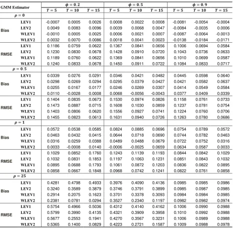
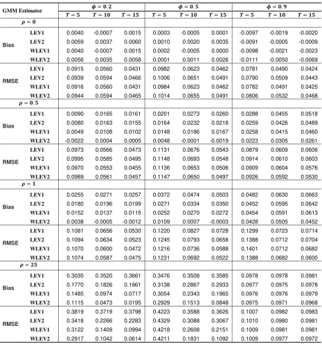
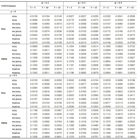
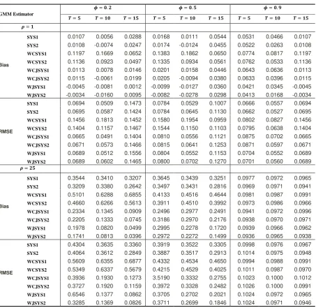
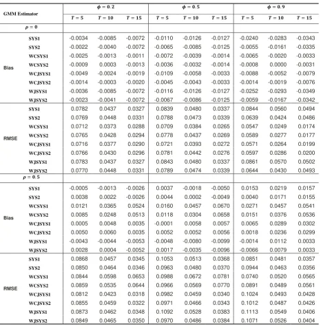
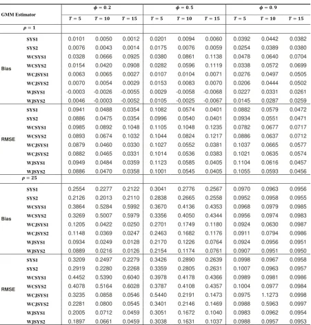
The results are given in Tables 1 to 6. Specifically, Tables 1 and 2 present the bias and RMSE of conventional and weighted level GMM estimators for the small, N = 50, and moderate, N = 100, samples, respectively. While Tables 3 to 6 present the bias and RMSE of conventional and weighted system GMM estimators, since Tables 3 and 4 dedicated for N = 50, while Tables 5 and 6 dedicated for N = 100.
From Tables 1 and 2, We can note that in case of 0, the bias and RMSE values for conventional level GMM (LEV1, LEV2) estimators equivalent to the bias and RMSE values for weighted level GMM estimators (WLEV1, WLEV2), the reason that when 0 lead to ̂ . Unless 0, WLEV2 estimator is smaller in bias and RMSE than other level GMM estimators, which indicates that the use of as a weighting matrix for level GMM estimator lead to improve the efficiency for this estimator. Moreover, the bias and RMSE for LEV1, LEV2, WLEV1, and WLEV2 estimators in Table 2 are smaller than the bias and MSE in Table 1 because the sample size was increased from 50 to 100.
From Tables 3 to 6, as in results level GMM estimation, we can note that in case of 0, the bias and RMSE values for SYS1 and SYS2 equivalent to the bias and RMSE values for WJSYS1 and WJSYS2. Moreover, WCSYS2 estimator is smaller in bias and RMSE (when 0 only) than other system GMM estimators. But when 0 1, we find that SYS2 and WJSYS2 are smaller in bias and RMSE than other system GMM estimators. Moreover, when 5, WCJSYS2 and WJSYS2 estimators are the smallest in bias and RMSE even in the case of increasing and is close to one. Moreover, the bias and RMSE for all system GMM estimators in Tables 5 and 6 are smaller than the bias and MSE in Tables 3 and 4 because the sample size was increased from 50 to 100.
V. CONCLUSION
We can summarize the main conclusions in the following points:
1. The bias and RMSE of all GMM estimators are increased with increasing by . While the bias and RMSE of weighted GMM estimators show a much slower increase whenever increased. Consequently, we conclude that the weighted GMM estimators are more efficiency than the conventional GMM estimators especially when 5.
2. In case of 0, the bias and RMSE values for the conventional level GMM (LEV1, LEV2) estimators equivalent to the bias and RMSE values for the weighted level GMM (WLEV1, WLEV2) estimators. Therefore, not any advantage of use the suggested weighting matrices in this case. While in system GMM estimation, when 0, the WCSYS2 estimator performs very well compared with other system GMM estimators.
3. In general, the WLEV2 and WJSYS2 estimators perform very well when compared with other level and system GMM estimators, respectively, in terms of bias and RMSE for all values of , , and . Theoretically, since system GMM estimation use many instruments about level GMM estimation, thus WJSYS2 estimator is more efficient than the WLEV2, which was confirmed by our simulation study. Consequently, we conclude that the WJSYS2 estimation will provide useful parameter estimates for the practitioner.
REFERENCES
[1] Abonazel, M. R., “Some Estimation Methods for Dynamic Panel Data Models”, PhD Thesis, Institute of Statistical Studies and
Research, Cairo University, 2014.
[2] Ahn, S. C., and Schmidt, P., “Efficient Estimation of Models for Dynamic Panel Data”, Journal of Econometrics, Vol. 68, pp. 5-28,
1995.
[3] Alvarez, J., and Arellano, M., “The Time Series and Cross-Section Asymptotics of Dynamic Panel Data Estimators”, Econometrica,
Vol. 71, pp. 1121-1159, 2003.
[4] Arellano, M., and Bond, S., “Some Tests of Specification for Panel Data: Monte Carlo Evidence and an Application to Employment
7
[5] Arellano, M., and Bover, O., “Another Look at the Instrumental Variable Estimation of Error-Components Models”, Journal of
Econometrics, Vol. 68, pp. 29-51, 1995.
[6] Blundell, R., and Bond, S., “Initial Conditions and Moment Restrictions in Dynamic Panel Data Models”, Journal of Econometrics,
Vol. 87, pp. 115-143, 1998.
[7] Bun, M., and Kiviet, J., “The Effects of Dynamic Feedbacks on LS and MM Estimator Accuracy in Panel Data Models”, Journal of
Econometrics, Vol. 132, pp. 409-444, 2006.
[8] Hayakawa, K., “Small Sample Bias Properties of the System GMM Estimator in Dynamic Panel Data Models”, Economics Letters, Vol. 95, pp. 32-38, 2007.
[9] Jung, H., and Kwon, H., “An Alternative System GMM Estimation in Dynamic Panel Models”, Hi-Stat Discussion Paper No. 217,
Hitotsubashi University, 2007.
[10] Newey, W., and Smith, R., “Higher Order Properties of GMM and Generalized Empirical Likelihood Estimators”, Econometrica, Vol.
72, pp. 219-255, 2004.
[11] Windmeijer, F., “Efficiency Comparisons for a System GMM Estimator in Dynamic Panel Data Models”, In Innovations in
Multivariate Statistical Analysis, Heijmans, R.D.H., Pollock, D.S.G. and Satorra, A., eds., A Festschrift for Heinz Neudecker, Advanced Studies in Theoretical and Applied Econometrics, Vol. 36, Kluwer Academic Publishers, Dordrecht (IFS working paper W98/1), 2000.
[12] Youssef, A. H., El-sheikh, A. A., and Abonazel, M. R., “Improving the Efficiency of GMM Estimators for Dynamic Panel Models”,
[image:8.595.68.533.286.740.2]Far East Journal of Theoretical Statistics, Vol. 47, pp. 171-189, 2014.
Table 1: Bias and RMSE for conventional and weighted level GMM estimators when N = 50
GMM Estimator
Bias
LEV1 -0.0007 0.0005 0.0026 0.0008 0.0022 0.0008 -0.0081 -0.0054 -0.0004
LEV2 0.0049 0.0083 0.0096 0.0039 0.0068 0.0047 -0.0084 -0.0035 0.0006
WLEV1 -0.0010 0.0005 0.0025 0.0006 0.0021 0.0007 -0.0087 -0.0064 -0.0013
WLEV2 0.0032 0.0070 0.0086 0.0018 0.0041 0.0023 -0.0138 -0.0184 -0.0171 RMSE
LEV1 0.1186 0.0759 0.0622 0.1367 0.0841 0.0656 0.1006 0.0694 0.0584
LEV2 0.1230 0.0830 0.0678 0.1428 0.0910 0.0720 0.1043 0.0736 0.0633
WLEV1 0.1189 0.0760 0.0622 0.1369 0.0841 0.0656 0.1010 0.0699 0.0587
WLEV2 0.1240 0.0833 0.0678 0.1450 0.0911 0.0722 0.1084 0.0833 0.0717
Bias
LEV1 0.0339 0.0276 0.0291 0.0346 0.0421 0.0482 0.0445 0.0598 0.0640
LEV2 0.0298 0.0269 0.0294 0.0295 0.0379 0.0427 0.0421 0.0582 0.0637
WLEV1 0.0255 0.0167 0.0177 0.0246 0.0269 0.0307 0.0414 0.0549 0.0584
WLEV2 0.0110 -0.0028 0.0008 0.0068 -0.0056 -0.0043 0.0377 0.0409 0.0339 RMSE
LEV1 0.1404 0.0835 0.0673 0.1530 0.0974 0.0826 0.1158 0.0761 0.0733
LEV2 0.1473 0.0887 0.0715 0.1608 0.1030 0.0859 0.1237 0.0781 0.0754
WLEV1 0.1403 0.0806 0.0620 0.1556 0.0927 0.0741 0.1224 0.0760 0.0706
WLEV2 0.1455 0.0823 0.0613 0.1631 0.0940 0.0726 0.1263 0.0780 0.0686
Bias
LEV1 0.0572 0.0538 0.0585 0.0824 0.0885 0.0696 0.0754 0.0789 0.0572
LEV2 0.0463 0.0432 0.0415 0.0644 0.0718 0.0690 0.0744 0.0782 0.0463
WLEV1 0.0316 0.0259 0.0388 0.0489 0.0488 0.0679 0.0722 0.0752 0.0316
WLEV2 0.0033 -0.0008 0.0140 -0.0006 -0.0025 0.0659 0.0634 0.0587 0.0033 RMSE
LEV1 0.1029 0.0852 0.1760 0.1243 0.1139 0.1193 0.0844 0.0842 0.1029
LEV2 0.1032 0.0831 0.1853 0.1197 0.1063 0.1231 0.0851 0.0843 0.1032
WLEV1 0.0895 0.0688 0.1793 0.1061 0.0872 0.1203 0.0836 0.0822 0.0895
WLEV2 0.0858 0.0667 0.1848 0.0968 0.0742 0.1241 0.0822 0.0761 0.0858
Bias
LEV1 0.4281 0.4798 0.4933 0.3976 0.4090 0.4136 0.0985 0.0985 0.0986
LEV2 0.3240 0.3589 0.3879 0.3746 0.3791 0.3899 0.0985 0.0987 0.0985
WLEV1 0.2914 0.2075 0.1623 0.3701 0.3378 0.3093 0.0984 0.0984 0.0985
WLEV2 0.2381 0.0781 0.0294 0.3527 0.2340 0.1197 0.0982 0.0982 0.0974 RMSE
LEV1 0.5754 0.4966 0.5036 0.4312 0.4140 0.4162 0.1006 0.0990 0.0988
LEV2 0.5799 0.3990 0.4135 0.4321 0.3909 0.3958 0.1010 0.0992 0.0988
WLEV1 0.5677 0.2553 0.1941 0.4270 0.3567 0.3231 0.1006 0.0989 0.0988
8
Table 2: Bias and RMSE for conventional and weighted level GMM estimators when N = 100
GMM Estimator
Bias
LEV1 0.0040 -0.0007 0.0015 0.0003 -0.0005 0.0001 -0.0097 -0.0019 -0.0020
LEV2 0.0059 0.0037 0.0060 0.0010 0.0020 0.0035 -0.0091 -0.0005 -0.0009
WLEV1 0.0040 -0.0007 0.0015 0.0002 -0.0005 0.0000 -0.0098 -0.0021 -0.0023
WLEV2 0.0056 0.0035 0.0058 0.0001 0.0011 0.0026 -0.0111 -0.0050 -0.0069 RMSE
LEV1 0.0915 0.0560 0.0431 0.0982 0.0623 0.0462 0.0781 0.0490 0.0424
LEV2 0.0939 0.0594 0.0466 0.1006 0.0651 0.0491 0.0790 0.0509 0.0443
WLEV1 0.0916 0.0560 0.0431 0.0984 0.0623 0.0462 0.0782 0.0491 0.0425
WLEV2 0.0944 0.0594 0.0465 0.1014 0.0655 0.0491 0.0806 0.0532 0.0468
Bias
LEV1 0.0090 0.0165 0.0161 0.0201 0.0273 0.0260 0.0288 0.0455 0.0518
LEV2 0.0080 0.0163 0.0155 0.0164 0.0232 0.0218 0.0259 0.0426 0.0489
WLEV1 0.0049 0.0108 0.0102 0.0148 0.0186 0.0167 0.0258 0.0415 0.0460
WLEV2 -0.0022 0.0004 0.0005 0.0048 -0.0001 -0.0019 0.0223 0.0305 0.0261 RMSE
LEV1 0.0973 0.0566 0.0473 0.1131 0.0676 0.0543 0.0879 0.0609 0.0606
LEV2 0.0995 0.0585 0.0495 0.1148 0.0693 0.0548 0.0914 0.0610 0.0603
WLEV1 0.0970 0.0553 0.0455 0.1136 0.0653 0.0506 0.0909 0.0604 0.0576
WLEV2 0.0989 0.0561 0.0457 0.1147 0.0650 0.0497 0.0926 0.0592 0.0530
Bias
LEV1 0.0255 0.0271 0.0257 0.0372 0.0474 0.0503 0.0482 0.0630 0.0663
LEV2 0.0180 0.0196 0.0199 0.0271 0.0334 0.0350 0.0452 0.0595 0.0642
WLEV1 0.0152 0.0137 0.0115 0.0252 0.0270 0.0272 0.0454 0.0591 0.0613
WLEV2 0.0038 -0.0005 -0.0012 0.0109 0.0007 -0.0003 0.0428 0.0505 0.0452 RMSE
LEV1 0.1081 0.0656 0.0530 0.1220 0.0827 0.0728 0.1299 0.0723 0.0714
LEV2 0.1094 0.0634 0.0523 0.1245 0.0793 0.0658 0.1388 0.0712 0.0704
WLEV1 0.1070 0.0600 0.0472 0.1216 0.0736 0.0588 0.1401 0.0712 0.0682
WLEV2 0.1074 0.0587 0.0475 0.1231 0.0692 0.0522 0.1388 0.0682 0.0600
Bias
LEV1 0.3035 0.3520 0.3661 0.3476 0.3508 0.3585 0.0978 0.0978 0.0981
LEV2 0.1770 0.1826 0.1961 0.3138 0.2867 0.2933 0.0977 0.0975 0.0978
WLEV1 0.1485 0.0974 0.0717 0.3054 0.2343 0.1965 0.0976 0.0976 0.0979
WLEV2 0.1115 0.0473 0.0195 0.2929 0.1513 0.0848 0.0975 0.0971 0.0968 RMSE
LEV1 0.3819 0.3719 0.3798 0.4223 0.3588 0.3626 0.1007 0.0982 0.0983
LEV2 0.3418 0.2266 0.2283 0.4329 0.3088 0.3067 0.1010 0.0980 0.0981
WLEV1 0.3122 0.1409 0.0994 0.4218 0.2608 0.2151 0.1009 0.0981 0.0981
9
Table 3: Bias and RMSE for conventional and weighted system GMM estimators when N = 50 and ρ = 0, 0.5
GMM Estimator
Bias
SYS1 -0.0139 -0.0164 -0.0145 -0.0227 -0.0227 -0.0235 -0.0332 -0.0541 -0.0558
SYS2 -0.0068 -0.0159 -0.0199 -0.0170 -0.0208 -0.0373 -0.0127 -0.0503 -0.0695
WCSYS1 -0.0086 -0.0050 -0.0010 -0.0172 -0.0056 -0.0032 -0.0107 -0.0082 -0.0040
WCSYS2 -0.0028 -0.0052 -0.0115 -0.0117 -0.0048 -0.0262 -0.0016 -0.0071 -0.0401
WCJSYS1 -0.0129 -0.0074 -0.0036 -0.0238 -0.0103 -0.0083 -0.0172 -0.0180 -0.0173
WCJSYS2 -0.0043 -0.0075 -0.0130 -0.0143 -0.0092 -0.0290 -0.0047 -0.0163 -0.0473
WJSYS1 -0.0144 -0.0165 -0.0146 -0.0239 -0.0229 -0.0236 -0.0369 -0.0573 -0.0580
WJSYS2 -0.0070 -0.0159 -0.0199 -0.0175 -0.0210 -0.0374 -0.0146 -0.0533 -0.0709
RMSE
SYS1 0.0989 0.0603 0.0476 0.1204 0.0669 0.0514 0.1095 0.0852 0.0732
SYS2 0.1041 0.0611 0.0591 0.1193 0.0664 0.0677 0.0929 0.0819 0.0905
WCSYS1 0.0905 0.0529 0.0405 0.1045 0.0528 0.0391 0.0744 0.0368 0.0248
WCSYS2 0.1038 0.0548 0.0536 0.1166 0.0542 0.0586 0.0834 0.0379 0.0627
WCJSYS1 0.0924 0.0538 0.0415 0.1078 0.0551 0.0412 0.0804 0.0431 0.0328
WCJSYS2 0.1045 0.0557 0.0545 0.1181 0.0562 0.0606 0.0863 0.0434 0.0687
WJSYS1 0.0993 0.0603 0.0476 0.1211 0.0671 0.0515 0.1143 0.0887 0.0754
WJSYS2 0.1042 0.0611 0.0591 0.1196 0.0665 0.0678 0.0954 0.0851 0.0918
Bias
SYS1 0.0103 -0.0062 -0.0052 0.0042 -0.0090 -0.0104 0.0233 0.0268 0.0196
SYS2 0.0179 -0.0058 -0.0145 0.0117 -0.0077 -0.0294 0.0115 0.0266 -0.0041
WCSYS1 0.0365 0.0655 0.0965 0.0360 0.0795 0.1122 0.0410 0.0632 0.0695
WCSYS2 0.0318 0.0616 0.0460 0.0317 0.0760 0.0411 0.0290 0.0623 0.0319
WCJSYS1 0.0103 0.0046 0.0069 0.0025 0.0076 0.0060 0.0128 0.0399 0.0417
WCJSYS2 0.0197 0.0044 -0.0073 0.0137 0.0080 -0.0197 0.0076 0.0394 0.0124
WJSYS1 0.0019 -0.0124 -0.0106 -0.0116 -0.0205 -0.0202 0.0017 0.0113 0.0040
WJSYS2 0.0143 -0.0116 -0.0178 0.0036 -0.0185 -0.0353 -0.0049 0.0112 -0.0160
RMSE
SYS1 0.1198 0.0639 0.0467 0.1377 0.0723 0.0506 0.1043 0.0574 0.0418
SYS2 0.1205 0.0645 0.0592 0.1342 0.0724 0.0678 0.1112 0.0572 0.0510
WCSYS1 0.1170 0.0928 0.1116 0.1292 0.1039 0.1243 0.0893 0.0683 0.0714
WCSYS2 0.1228 0.0902 0.0764 0.1369 0.1018 0.0749 0.1075 0.0681 0.0520
WCJSYS1 0.1122 0.0602 0.0453 0.1299 0.0694 0.0480 0.1266 0.0665 0.0555
WCJSYS2 0.1208 0.0614 0.0569 0.1379 0.0705 0.0629 0.1309 0.0666 0.0527
WJSYS1 0.1214 0.0654 0.0475 0.1449 0.0765 0.0543 0.1348 0.0713 0.0488
10
Table 4: Bias and RMSE for conventional and weighted system GMM estimators when N = 50 and ρ = 1, 25
GMM Estimator
Bias
SYS1 0.0107 0.0056 0.0288 0.0168 0.0111 0.0544 0.0531 0.0466 0.0107
SYS2 0.0108 -0.0074 0.0247 0.0174 -0.0124 0.0455 0.0522 0.0263 0.0108
WCSYS1 0.1197 0.1669 0.0652 0.1383 0.1862 0.0650 0.0774 0.0817 0.1197
WCSYS2 0.1136 0.0923 0.0497 0.1335 0.0934 0.0561 0.0762 0.0533 0.1136
WCJSYS1 0.0113 0.0078 0.0146 0.0201 0.0158 0.0446 0.0643 0.0636 0.0113
WCJSYS2 0.0115 -0.0061 0.0199 0.0205 -0.0094 0.0380 0.0633 0.0396 0.0115
WJSYS1 -0.0045 -0.0081 0.0012 -0.0099 -0.0127 0.0360 0.0421 0.0345 -0.0045
WJSYS2 -0.0034 -0.0160 0.0095 -0.0082 -0.0278 0.0298 0.0413 0.0168 -0.0034
RMSE
SYS1 0.0694 0.0509 0.1473 0.0784 0.0529 0.1007 0.0666 0.0557 0.0694
SYS2 0.0695 0.0587 0.1424 0.0784 0.0645 0.1130 0.0662 0.0527 0.0695
WCSYS1 0.1456 0.1813 0.1452 0.1580 0.1954 0.0959 0.0802 0.0827 0.1456
WCSYS2 0.1404 0.1157 0.1467 0.1544 0.1150 0.1103 0.0795 0.0638 0.1404
WCJSYS1 0.0665 0.0491 0.1404 0.0810 0.0556 0.1121 0.0875 0.0702 0.0665
WCJSYS2 0.0671 0.0573 0.1466 0.0815 0.0641 0.1253 0.0871 0.0597 0.0671
WJSYS1 0.0689 0.0512 0.1556 0.0804 0.0552 0.1153 0.0704 0.0552 0.0689
WJSYS2 0.0689 0.0602 0.1465 0.0800 0.0702 0.1270 0.0701 0.0560 0.0689
Bias
SYS1 0.3544 0.3410 0.3207 0.3645 0.3439 0.3251 0.0977 0.0972 0.0965
SYS2 0.3209 0.3380 0.2642 0.3497 0.3431 0.2816 0.0969 0.0971 0.0941
WCSYS1 0.5101 0.6288 0.6855 0.4133 0.4516 0.4644 0.0981 0.0987 0.0991
WCSYS2 0.4660 0.6266 0.5613 0.3911 0.4510 0.3992 0.0973 0.0986 0.0966
WCJSYS1 0.2334 0.1345 0.0909 0.2496 0.2977 0.2491 0.0941 0.0972 0.0996
WCJSYS2 0.2205 0.1333 0.0745 0.3186 0.2970 0.2176 0.0938 0.0970 0.0971
WJSYS1 0.1978 0.0820 0.0499 0.2995 0.2278 0.1720 0.0939 0.0966 0.0962
WJSYS2 0.1741 0.0813 0.0396 0.2972 0.2272 0.1499 0.0936 0.0965 0.0938
RMSE
SYS1 0.4304 0.3635 0.3360 0.3919 0.3522 0.3305 0.0998 0.0976 0.0967
SYS2 0.4064 0.3612 0.2849 0.3887 0.3517 0.2913 0.1014 0.0975 0.0948
WCSYS1 0.5609 0.6355 0.6877 0.4332 0.4534 0.4650 0.0994 0.0988 0.0991
WCSYS2 0.5349 0.6337 0.5679 0.4215 0.4529 0.4025 0.1011 0.0987 0.0970
WCJSYS1 0.3936 0.1930 0.1273 3.5190 0.3332 0.2755 0.1023 0.1000 0.1012
WCJSYS2 0.3727 0.1920 0.1159 0.3972 0.3328 0.2482 0.1026 0.1000 0.0991
WJSYS1 0.6546 0.1377 0.0862 0.3705 0.2702 0.2021 0.1024 0.0972 0.0965
11
Table 5: Bias and RMSE for conventional and weighted system GMM estimators when N = 100 and ρ = 0, 0.5
GMM Estimator
Bias
SYS1 -0.0034 -0.0085 -0.0072 -0.0110 -0.0126 -0.0127 -0.0240 -0.0283 -0.0343
SYS2 -0.0022 -0.0040 -0.0072 -0.0065 -0.0085 -0.0125 -0.0055 -0.0161 -0.0335
WCSYS1 -0.0025 -0.0013 -0.0011 -0.0072 -0.0039 -0.0014 -0.0065 -0.0020 -0.0033
WCSYS2 -0.0009 0.0003 -0.0013 -0.0036 -0.0032 -0.0014 -0.0008 0.0000 -0.0031
WCJSYS1 -0.0049 -0.0024 -0.0019 -0.0109 -0.0058 -0.0033 -0.0088 -0.0052 -0.0079
WCJSYS2 -0.0014 -0.0003 -0.0020 -0.0045 -0.0043 -0.0033 -0.0014 -0.0019 -0.0076
WJSYS1 -0.0036 -0.0085 -0.0072 -0.0116 -0.0126 -0.0127 -0.0252 -0.0293 -0.0349
WJSYS2 -0.0023 -0.0041 -0.0072 -0.0067 -0.0086 -0.0125 -0.0059 -0.0167 -0.0342
RMSE
SYS1 0.0782 0.0437 0.0327 0.0839 0.0480 0.0337 0.0844 0.0560 0.0494
SYS2 0.0769 0.0448 0.0331 0.0788 0.0473 0.0339 0.0639 0.0424 0.0486
WCSYS1 0.0712 0.0373 0.0288 0.0709 0.0384 0.0265 0.0547 0.0249 0.0174
WCSYS2 0.0765 0.0428 0.0294 0.0778 0.0437 0.0269 0.0589 0.0277 0.0177
WCJSYS1 0.0716 0.0377 0.0290 0.0721 0.0393 0.0272 0.0571 0.0264 0.0199
WCJSYS2 0.0766 0.0430 0.0296 0.0781 0.0442 0.0276 0.0597 0.0286 0.0200
WJSYS1 0.0783 0.0437 0.0327 0.0843 0.0480 0.0337 0.0861 0.0570 0.0502
WJSYS2 0.0770 0.0448 0.0331 0.0789 0.0474 0.0339 0.0644 0.0430 0.0493
Bias
SYS1 -0.0005 -0.0013 -0.0026 0.0037 -0.0018 -0.0050 0.0153 0.0219 0.0157
SYS2 0.0038 0.0022 -0.0026 0.0044 0.0002 -0.0049 0.0040 0.0171 0.0155
WCSYS1 0.0121 0.0365 0.0524 0.0160 0.0457 0.0670 0.0271 0.0457 0.0541
WCSYS2 0.0085 0.0248 0.0513 0.0118 0.0304 0.0658 0.0151 0.0376 0.0536
WCJSYS1 0.0005 0.0048 0.0035 -0.0001 0.0058 0.0057 0.0065 0.0289 0.0302
WCJSYS2 0.0050 0.0060 0.0035 0.0052 0.0052 0.0056 0.0018 0.0236 0.0299
WJSYS1 -0.0043 -0.0044 -0.0053 -0.0048 -0.0080 -0.0099 -0.0014 0.0112 0.0033
WJSYS2 0.0028 0.0004 -0.0052 0.0017 -0.0035 -0.0096 -0.0066 0.0079 0.0033
RMSE
SYS1 0.0868 0.0457 0.0345 0.1053 0.0513 0.0368 0.0851 0.0481 0.0357
SYS2 0.0850 0.0464 0.0346 0.0963 0.0480 0.0370 0.0944 0.0463 0.0356
WCSYS1 0.0844 0.0598 0.0653 0.0988 0.0672 0.0781 0.0740 0.0520 0.0565
WCSYS2 0.0859 0.0535 0.0644 0.0966 0.0569 0.0770 0.0891 0.0489 0.0561
WCJSYS1 0.0812 0.0423 0.0318 0.0982 0.0459 0.0340 0.1024 0.0493 0.0428
WCJSYS2 0.0855 0.0459 0.0322 0.0971 0.0466 0.0343 0.1012 0.0487 0.0426
WJSYS1 0.0873 0.0462 0.0348 0.1092 0.0528 0.0383 0.1113 0.0549 0.0406
12
Table 6: Bias and RMSE for conventional and weighted system GMM estimators when N = 100 and ρ = 1, 25
GMM Estimator
Bias
SYS1 0.0101 0.0050 0.0012 0.0201 0.0094 0.0060 0.0392 0.0442 0.0382
SYS2 0.0076 0.0043 0.0014 0.0175 0.0076 0.0059 0.0254 0.0389 0.0380
WCSYS1 0.0328 0.0666 0.0925 0.0380 0.0861 0.1138 0.0478 0.0640 0.0704
WCSYS2 0.0154 0.0420 0.0908 0.0282 0.0596 0.1119 0.0338 0.0572 0.0699
WCJSYS1 0.0063 0.0065 0.0027 0.0107 0.0104 0.0071 0.0276 0.0497 0.0505
WCJSYS2 0.0070 0.0054 0.0029 0.0153 0.0083 0.0070 0.0206 0.0444 0.0502
WJSYS1 -0.0003 -0.0026 -0.0055 0.0029 -0.0058 -0.0068 0.0227 0.0331 0.0261
WJSYS2 0.0046 -0.0003 -0.0052 0.0105 -0.0025 -0.0067 0.0145 0.0287 0.0259
RMSE
SYS1 0.0941 0.0488 0.0354 0.1082 0.0574 0.0401 0.0882 0.0579 0.0472
SYS2 0.0886 0.0475 0.0354 0.0996 0.0540 0.0401 0.0934 0.0551 0.0471
WCSYS1 0.0985 0.0892 0.1048 0.1105 0.1048 0.1235 0.0782 0.0677 0.0717
WCSYS2 0.0893 0.0674 0.1032 0.1044 0.0824 0.1217 0.0886 0.0637 0.0712
WCJSYS1 0.0879 0.0460 0.0330 0.1027 0.0552 0.0381 0.1037 0.0665 0.0577
WCJSYS2 0.0882 0.0465 0.0331 0.1014 0.0536 0.0383 0.1021 0.0635 0.0574
WJSYS1 0.0949 0.0484 0.0359 0.1123 0.0585 0.0405 0.1104 0.0616 0.0457
WJSYS2 0.0886 0.0470 0.0358 0.1001 0.0545 0.0405 0.1055 0.0593 0.0456
Bias
SYS1 0.2554 0.2277 0.2122 0.3041 0.2776 0.2567 0.0970 0.0963 0.0956
SYS2 0.2126 0.2013 0.2110 0.2838 0.2665 0.2558 0.0952 0.0958 0.0955
WCSYS1 0.3864 0.5284 0.5992 0.3670 0.4136 0.4353 0.0968 0.0979 0.0985
WCSYS2 0.3269 0.5007 0.5979 0.3356 0.4050 0.4344 0.0956 0.0974 0.0983
WCJSYS1 0.1205 0.0422 0.0250 0.2701 0.1749 0.1180 0.0924 0.0630 0.0987
WCJSYS2 0.1148 0.0369 0.0247 0.2463 0.1682 0.1176 0.0911 0.0794 0.0986
WJSYS1 0.0934 0.0249 0.0128 0.2170 0.1226 0.0764 0.0924 0.0956 0.0951
WJSYS2 0.0889 0.0216 0.0126 0.2154 0.1174 0.0761 0.0907 0.0951 0.0950
RMSE
SYS1 0.3209 0.2497 0.2279 0.3426 0.2890 0.2639 0.0998 0.0967 0.0958
SYS2 0.2919 0.2280 0.2268 0.3359 0.2805 0.2631 0.1007 0.0963 0.0957
WCSYS1 0.4452 0.5390 0.6040 0.3978 0.4178 0.4366 0.0989 0.0981 0.0986
WCSYS2 0.4078 0.5164 0.6028 0.3787 0.4108 0.4357 0.1004 0.0977 0.0984
WCJSYS1 0.3235 0.0858 0.0546 0.5440 0.2191 0.1473 0.0975 1.1273 0.0998
WCJSYS2 0.2281 0.0800 0.0545 0.3401 0.2146 0.1469 0.0988 0.5963 0.0997
WJSYS1 0.2005 0.0712 0.0459 0.3051 0.1672 0.1040 0.0983 0.0962 0.0954