The Solution Classical Feedback Optimal Control Problem for m Persons Differential Game with Imperfect Information

(1)

The Solution Classical Feedback Optimal Control Problem

for m-Persons Differential Game with Imperfect

Information

Jaykov Foukzon1, Elena Men’kova2, Alex Potapov3 1

Department of Mathematics, Israel Institute of Technologies, Haifa, Israel 2

All-Russian Research Institute for Opto-Physical Measurements, Moscow, Russia 3

V.A. Kotel’nikov Institute of Radio Engineering and Electronics, Russian Academy of Sciences, Moscow, Russia Email: [email protected], [email protected], [email protected]

Received January 12, 2013; revised February 11, 2013; accepted March 5, 2013

ABSTRACT

The paper presents a new approach to construct the Bellman function 

 

t x, and optimal control directly by way of using strong large deviations principle for the solutions Colombeau-Ito’s SDE. The generic imperfect dynamic models of air-to-surface missiles are given in addition to the related simple guidance law. A four examples have been illustrated, corresponding numerical simulations have been illustrated and analyzed.

 

,

u t x

Keywords: Optimal Control; Bellman Equation

1. Mathematical Challenge: Creating

a Game Theory That Scales

What new scalable mathematics is needed to replace the traditional Partial Differential Equations (PDE) approach to differential games?

Let be a probably space. Any stochastic

process on is a measurable mapping



  , ,

d







: 0,

X T 

 

,

u t x

n

 . Many stochastic optimal control

problems essentially come down to constructing a function that has the properties

1)

 

, inf



,

   

,



x t D

u t x  _E J X_   t _,

2)

 





,

 



_{ }

' 0,

, inf x

s D ,

s t

u t x _E J X







 _



 



_{' 0,}_{ }





, ',

 



,

x t D

s t ',

s _ u t x t t

   _ 

n



 

t U U,

  _ , where J is the termination payoff

functional, 



t



is a control and



_,



is some

0

x t D

t

x 

Markov process governed by some stochastic Ito’s equation driven by a Brownian motion of the form

3) ,

 

₀



,

   

,



d

 

,

t

x x

t D s D

x   x



g x   t s DW t  ,

where W t



,



is the Brownian motion. Traditionally the function u t x

 

, has been computed by way of solving the associated Bellman equation, for which vari- ous numerical techniques mostly variations of the finite difference scheme have been developed. Another ap-

proach, which takes advantage of the recent develop- ments in computing technology and allows one to construct the function u x t

 

, by way of backward induc- tion governed by Bellman’s principle such that described in [1]. In paper [1] Equation (3) is approximated by an equation with affine coefficients which admits an explicit solution in terms of integrals of the exponential Brow- nian motion. In approach proposed in paper [2,3] we have replaced Equation (3) by Colombeau-Ito’s Equation (4)











  



 





 

, ,

, , , ₀ , , ,

, ,

t

x x

t D s D , d

,

x x g x t s

D w t w t

 

 _  

 _

    

  

 _  



 _

 

 







', 0,1 ,

   1, 2, where w t



,



is th e

white noise on n, i.e.,

 

, d



d

w t W t

t ,



   almost

surely in D', and w__'

 

t, is the smoothed white noise on n i.e.,

 





' , , , '

w_ t  w t _ s t ,

and ' is a model delta net [2,4]. Fortunately in

con-trast with Equation (3) one can solve Equation (4) with-out any approximation using strong large deviations principle [4]. In this paper we considered only quasi sto-chastic case, i.e. D0,0. General case will be con-sidered in forthcoming papers.

(2)

posed idea: A new approach, which is proposed in this paper allows one to construct the Bellman function

and optimal control directly, i.e., without any reference to the Bellman equation, by way of using strong large deviations principle for the solutions Colombeau-Ito’s SDE (CISDE).



,

V t x







t x,



2. Proposed Approach

Let us consider an m-persons Colombeau-Ito’s differen-

tial game ;



, , ,

 

n m T

CDG f g y G



with a stochastic nonlinear dynamics:

 







 



 



 





, , ,

, , , 0,1

x t f t x t Dw t t

w t  _    _        _    _       ;

 

0, :



 



,

 

0 0,

 

,

n

t T x_ t x x f f_ _



   

    _{ } _ _

 

, ,

 

n ,

g g_{ }  f gG (1)

 



1

 

, ,

 



,

 

i, 1, , ,

k

m i i

t t t t U i

   _     _ m



and m-persons Colombeau-Ito’s differential game with imperfect infor-mation about the system [5-8]:

 



; , , , ,

n m T

CIDG f g y G  t

 





 





 



 











 





, , , , ,

, , , 0,1

x t

f t x t Dw t t t t

w t  _    _          _    _       ;

 

0, :



 



,

 

0 0,

 

,

n

t T x_ t x x f f_ _



   

    _{ } _ _

 

, ,

 

n ,

g g_{ }  f gG (2)

 



1

 

, ,

 



,

 

i, 1, , ,

k

m i i

t t t t U i

   _      m



Here is the algebra of Colombeau generalized

functions [9], is the ring of Colombeau’s generalized numbers [10-12],



n

G



n _{  }

 _{  } ; ti

 

t is

the control chosen by the i-th player, within a set of ad-missible control values , and the playoff for the i-th player is: i U

 



 





1 2 1 2

, , ,1

0 1 2 , 1 , , ,

, , d

T i i m n i i i

,n ;

J E E g t x t x t

t t t

E E x T y

   _      _       _         _       _          _       _ _  _ _ _  _ __   









 . (3)

where is the trajectory

of the Equation (1). Optimal control problem for the i-th player is:

 







 





,1 , , ,n _'



t x t __  x t

 

_{ }

 ,

, min max

i j t j i

i

t

J _ _ _ J ,i

     _              

 . (4)

Let us consider now a family

 

,

t x 

 

 of the

solu-tions Colombeau-Ito’s SDE:

 



 



 

 





, , , 0 0 , ;

, 0, , , 0,1

t t

n

d x b x t dW t

x x t T

       _            _          (5)

where W t

 

is n-dimensional Brownian motion,

 

, 0

 

, :

n _b _t n

   

b G

  _ n

   is a polynomial,

i.e.

 





0, 0, 1

0

, ,

, 1, , .

i

i k

k j j

b x t b t x i i

i i n

     _     , , ,



 

Definition 1. CISDE (5) is -dissipative if exist

Lyapunov candidate function and Colombeau





,

V xt



constants 

 

C   C 0,



r



r, such that:

1)  

 

0,1 ,



0,1 ,



x x, r: V x t b



, ; 



  C V x t

 

, ;





 

,

 

1 , , , ; , n i i i

V x t V x t

V x t b b x

t x       



 

2) r

 

lim inf

 

r x r

V x V x

 

 

   

  .

Theorem 1. Main result (strong large deviations principle) [5,13]. For any solution xt



x1,t, ,xn,t



 _  

 of dis-

sipative CISDE (5) and valued parameters 1,,n, there exist Colombeau constant

 

,

 

0

C C R C    ,

such that  , 



1,,n



:

 

2 2

, 0

lim infE x_t  C U t,

  _ 



 _

_  _ _ _ _

_ _ __ 

  . (6)

where a function U t

 

, 



U t1

 

, ,,Un

 

t,



is the solution of the master equation:

 

,

 

,

   

, , 0, 0

U t  J b_  t _Ub  t U  x , (7) where J J b_

 

,t _ the Jacobian, i.e. J is a n n - matrix:

 

, 0,i

 

, j

J b  t    b x t x  x .

Remark.1. We note that   



0,1 :



 







, 0,



0

lim inf _t _t 0

t E x  x 

 _ _      _ _    . Example 1.

   

 

 

3 2 0 sin

, 1, 0 , 0 , 0,

n m

t t t t

k

x a x b x cx t t t

W t a x x t T

(3)

From a general master Equation (7) one obtain the next linear master equation:

 





 





 

2 3

0

3 2

sin , 0

n m k

u t a b c u t a b c

t t t u x

2                        

. (8)

From the differential master Equation (8) one obtain transcendental master equation

 







 







 





 









2 0 3 2 0 2

exp 3 2

sin

exp 3 2 d 0

t

n m

x t a t b t t

a t b t

a t b t t

               _   _          _   _ 



. (9)

Numerical simulation: Figures 1 and 2.

   

 

 

0

3 2

0 0 0 0

0

1, 5, 1, 2, 2, 0,

5, 0.01,

sin , 0 , 0,

n

t t t t

m k

a b c m n x

T R T

x a x b x cx t

t t x x t T

                          

 . (10)

Here

 

0 2

0

lim inf _t _t .

t E x x

    _  



Let us consider now

an m-persons Colombeau stochastic differential game with nonlinear dynamics

 



; , , ,

n m T

CDG f g y G

 







 



 



 





 

 





 



 



 



 



 

, , , 0 1 1 , , , ,

: , 0 , 0, , 0,1

, , , , 1, , .

i i

n

k

m i i

k

m i i

;

, 1,

x t f t x t t dW

t x t x x t T

t t t t U i m

  _    _ _   _               _   _ _  _                     t    (11) Here n     , ti

 

t is the control chosen

by the i-th player, within a set of admissible control val-ues Ui, and the playoff of the i-th player is

 



   











, , , 0 2 , ; 1

, ; d

, T i i n i i i

J E g x t t t

E x T y

  _    _   _     _   _  _          _    _





_  _   (12)

where y



y1,,yn



and tx t



,



is the

trajec-tory of the Equation (11). Theorem 2.For any solution





 



















 



, , ,

1, , 1

,

, , , , ,

t

t n t m

X t





X X t

                     

  t

of the dissipative ;



, 0, ,

 

and

n m T

[image:3.595.308.539.84.153.2]

CDG f y G



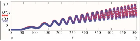
val-

Figure 1. The solution of the Equation (8) in a comparison with a corresponding solution x t of the ODE (10).

 

Figure 2. 

 

r versus R.

ued parameters 1,,n, there exists Colombeau constant C

 

C_ _ ,

 

C_ _ 0, such that:





 

1 2 2 , 0 , , ,

lim inf ,

n

t

E x  C U t

 _         _   _  _ _ _ _       

. (13)

where U t

 

, 



U t1

 

, ,,Un

 

t,



the trajectory of the corresponding master game

 







 



 

0

,

, , , , , 0,

,

U t

J f t U f t U

x             _ _      

 

2

i

J  U T (14)

Example 2.

1) 3

 

1 2, 2 2 1 2 ,

x x x  kx  t  t k0,

 





 





1 t 1, 1 , 2 t 2, 2 ,

       

 

 

1 01 2

2 2

1 2

0, , 0 , 0 ;

, 1, 2; i

t T x x x x

J x T x T i

 

  

02 

optimal control problem for the first player:

     

 

1 1 2 2 2 2

2 2

1 2

, ,

min max

t t x T x T

       

 _ _ _

 _ _

 

and optimal control problem for the second player:

   1   1 1

 

2

2 2

1 2

, ,

max min .

u u t

t    x T x T

     

 _ _ _

 _ _

 

From Equation (14) we obtain corresponding master game:

(4)

 





 





 

1 1 1 2 2 2 1 01

2 2

2 02 2 1 2

, , , , 0

0 ; i , 1, 2;

t t u

u x J u T u T i

1, x

      



     

    

 

optimal control problem for the first player is:

     

 

1 1 2 2 2 2

2 2

1 2

, ,

min max

t t u T u T

       

 _ _ _

 _ _

 

 

and optimal control problem for the second player is:

   1  1 1

 

2

2 2

1 2

, ,

max min .

u u t

t    u T u T

     

 _ _ _

 _ _

 



Having solved by standard way [14,15] linear master game (2) one obtain optimal feedback control of the first player:

 

   

 

1 1 1 2

1 1 2

, ,

sign

t t x t x t

x t _ t x

 



 

 

 

  _  _ _ _



t

and optimal feedback control of the second player [5]:

 

   

 

   

2 2 1 2

2 1 2

, ,

sign .

t t x t x t

x t _ t x t

 



 

 

  _   _



Here _

 

t  _



_

 

t



,_

 

t t,

 

t t ceil t 1 ,







   

_ _{ } _  

 

where ceil

 

x is a part-whole of a number x . Thus, for numerical simulation we obtain ODE:

 

1 2 ,

x t x t

 

   

 

   

3

2 2 1 1 2

2 1 2

sign

sign .

x t kx t x t t x t

x t t x t



 

    _   _

  _   _



Numerical simulation: Figures 3-6

 





1

1 2

2 2

1, 400, 100, 5,

0 300 m, 0 30 m sec ,

80 sec, sin .

k A

x x

T t A t

 

 

   

 

  

Theorem 3. For any solution





 



















 







,

, ,

1, , 1

,

, , , , ,

t

t n t m

X t

X X t

  

   

 



 

 





 

[image:4.595.337.510.84.195.2]

  t

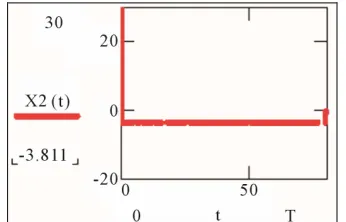
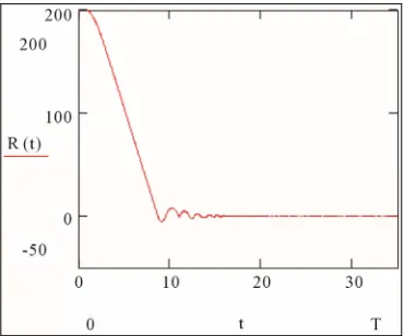
Figure 3. Optimal trajectory: x t₁

   

x T₁ 0.4 m.

[image:4.595.338.507.231.346.2]

Figure 4. Optimal velocity: x t₂

 

x T₂

 

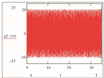
 0.4 m sec/ .

Figure 5. Optimal control of the first player.

Figure 6. Control of the second player.

of the dissipative ;



, 0, ,

 

,



n m T

CIDG f y G  and

valued parameters 1,,n, there exists Colombeau constant _C

 

_C_ _,

 

_C_

  0,

 

_  _   such that:

 

2 2

0

lim infE x_t C U t,

  

 _ _ _

 

  . (15)

where U t

 

, 



U t1

 

, ,,Un

 

t,



the trajectory of the corresponding master game

 



 



 



 



 









0

, , ,

, , , 0,

,

U t J f w t t t U

f w t t t U

x

    



    



 

 _   _

  

 

 

 ₍₁₆₎

 



 



 

1 2

, , , , 1, , ,

.

i

k

m i i

i

t t t t U R i

J U T

     



m



  _   _ _

[image:4.595.60.270.357.714.2]

(5)

1) x t1

 

x2

 

t ,

 

   

 

   





 





 





3 2

2 1 2 2 2

1 1 2

2 1 2 1 2

1 1 1 2 2 2

, ,

, , , 0, ,

, , , ,

x t k x t k x t

t x t x t t

t x t x t k k

t t

 



     

  

 _  _

 _ _  

   



,  

 

2 2

1 1 , 1, 2

i

J x T x_ T i . From Equation (16) one

obtain corresponding master game: 2) u1u22,





   

 

   

 





 





 

2 3

2 1 2 2 2 2 1 2 2

1 1 2

2 1 2

1 1 1 2 2 2

2 2

1 2

3 2

, ,

, , ,

, , , ,

, 1, 2. i

u k k u k k

t u t u t t

t u t u t

t t

J u t u t i

2 2

  

 



     

    

 _  _

 _ _

   

  

  

 



Having solved by standard way linear master game (2) one obtain local optimal feedback control of the first player [5]:

 



  



 



1 t 1sign x t1 tn1 t x2 t

  



 

  _    t _

t

and local optimal feedback control of the second player:

 

  

  

2 t 2sign x t1 tn1 t x2 .

 





  _   _



t 

t

Thus, finally we obtain global optimal control of the next form [5]:

 

   



 

   

1 1 1 2

2 2 1 2

sign ,

sign .

t x t t x t

t x t t x t



  

 





  _   

 _   _

Here _

 

t  _



_

 

t



,_

 

t  ,

 

t t ceil t 1 ,







   

_ _{ } _  

 

where ceil x

 

is a part-whole of a number x . Thus, for numerical simulation we obtain ODE: x1x2,

 

   



 



 

   

2 1 2 2 2 1 1 2

2 1 2 .

3 2

x k x k x sign x t t x t t

sign x t t x t



 



 

     _    _

  _   _



Numerical simulation: Figures 7-12. Game with imperfect measurements: red curves x t1

   

,x2 t . Classical

game: blue curves y t1

   

,y2 t .

 





t



2

sin

t A

  .

3. Homing Missile Guidance with Imperfect

Measurements Capable to Defeat in

Conditions of Hostile Active

Radio-Electronic Jamming

Homing missile guidance strategies (guidance laws) dic-tate the manner in which the missile will guide to inter-cept, or rendezvous with, the target. The feedback nature of homing guidance allows the guided missile (or, more

generally, the pursuer) to tolerate some level of (sensor) measurement uncertainties, errors in the assumptions used to model the engagement (e.g., unanticipated target maneuver), and errors in modeling missile capability (e.g., deviation of actual missile speed of response to guidance commands from the design assumptions). Nev-ertheless, the selection of a guidance strategy and its subsequent mechanization are crucial design factors that can have substantial impact on guided missile perform-ance. Key drivers to guidance law design include the type of targeting sensor to be used (passive IR, active or semi-active RF, etc.), accuracy of the targeting and iner-tial measurement unit (IMU) sensors, missile maneuver-ability, and, finally yet important, the types of targets to be engaged and their associated maneuverability levels.

Figure 13 shows the intercept geometry of a missile in planar pursuit of a target. Taking the origin of the refer-ence frame to be the instantaneous position of the missile, the equation of motion in polar form are [16]:

   

 

   

 

2

, , ,

, , , .

2 , ,

, , ,

r r

M T

r r r r r

M M M T T T

n n

M T

n n n n n

M M M T T T

R R a t R t R t a t

a t a a a t a a

R R a t t t a t

a t a a a t a a



    ,

. r

n

 

  __ __

  

 _ _  _ 

 

  _ _



  

 _ _  _ 

  _  

 

   



(17)

1) The variable RR t

 

denotes a true target-to- missile range TM

 

2)The variable

R t .

 

RR t denotes the it is real meas-ured target-to-missile range RTM

 

t .

3) The variable  

 

t denotes a true line-of-sight angle (LOST) i.e., the it is true angle between the con-stant reference direction and target-to-missile direction.

4)The variable   

 

t denotes the it is real meas- uredline-of-sight angle (LOSM) i.e., the it is true angle between the constant reference direction and target-to- missile direction.

5) The variable a_Mn

 

t a_Mn _t R t,

   

,R t _ denotes the missiles acceleration along direction which perpen-dicularly to line-of-sight direction.

6) The variable aMr

 

t aMr t,

 

t ,

 

t  denotes the missile acceleration along target-to-missile direction.

7)The variable aTn

 

t denotes the target acceleration along direction which perpendicularly to line-of-sight direction.

8) The variable aTr

 

t denotes the target acceleration along target-to-missile direction.

Using replacement z_R into Equation (17) one obtain:

   

 

2

, , ,

r r

M T

r r r r r

M M M T T

z

R a t R t R t a t

R

a t a a a t a a

 

  __ __

. r T

  

 _ _  _ 

 _

  



(6)

[image:6.595.76.528.65.725.2]

Figure 7. Uncertainty of speed measurements 

 

t .

Figure 8. Cutting function

 

11.

. 10

t 

[image:6.595.334.509.76.386.2]

 

Figure 9. Optimal trajectory.

[image:6.595.337.509.85.216.2]

Figure 10. Optimal velocity.

Figure 11. Optimal control of the first player.

Figure 12. Optimal control of the second player.

Figure 13. Planar intercept geometry.

   

 

, , ,

r n

M T

n n n n n

M M M T T

Rz

z a t z t z t a t

R

a t a a a t a a

 

  _ _

. n T

  

 _ _  _ _

  _

  

(18)

 

   

 

   

,

.

z t R t t

z t R t t R t t



 



 

 

 _



   

 _ _

 

Suppose that:

 

1

   

,

 

2

 

.

R t R t  t  t  t  t

[image:6.595.81.265.85.237.2] [image:6.595.84.264.420.725.2]

(7)

 

1

 

1

 

, 1

 

.

R t R t  t R t  t  ₁ t

 

t

 

t 2

   

t , t

 

t 2



.

_ _  _ _  t



 

   



 





 



   



 



   

 

   



 



   

 

1 2 1 2

1 2 2

2 ,

z t R t t R t t t t

R t t t t t R t t

z t t t t R t t

z t t

                     _   _   _   2        _ _             

 

   



 



   

2 t 1 t t 2 t R t 2 .

  _     t (20)

 

   

 







 



 







 



   



 



   



 



 

   



 



 

   



 



1 2 1 2 1 2

2 2 1 2

3

3 2 2 1 2

,

.

z t R t t R t t

R t t t t

R t t R t t t t t

z t R t t R t t t t t

z t t

t R t t R t t t t t

                                        _  _                     _ _     _      _ _ _     _  _ _ _   _    _ _ _   _

Let us consider antagonistic Colombeau differential

game



 

2



2;T , 0, , , , ,

IDG f y G  w



1, 2, 3, 4



,

      w



 2, 4



with non-linear

dy-namics and imperfect measurements [6]:

 

   

 

   

 

2 3 1 1 2 , , , , ; , , , , . r r r

r M T

r r

M M r r

r r

r r r r r r

M M M T T T

R V

z

V a t a t

R

a t a t R t V t k V t

R t R t t V t V t t

a t a a a t a a

         _ _          _ _  _ _          ,

zw (21)

 

   



 



   

     

 

3 2 3 4 2 1 , , , , , , , ,

, 1, 2.

n n

r

M T

n n

M M

n n n n n

M M M T T T

i

V w

w a t a t

R

a t a t w t w t k w t

z t z t t z t z t t

a t a a a t a a

J R t i

         _ _         _ _  _               , . n 

Optimal control problem of the first player is:

       

 

1 , , , 2 1 , , , min max .

r r n n n

M M M M M M

r r r n n n

T T T T T T

S t a a a t a a

a t a a a t a a

J R t       _ _  _ _      _ _  _ _            (22)        

 

2 max , , , 2 1 , , , min

Optimal control problem of the second player is:

.

r r r n n n

J

   

T T T T T T

r r r n n n

M M M M M M

a t a a a t a a

R t  _ _  _ _      _ _  _ _            (23)

From Equations (21)-(23) one obtain corresponding linear master game:

 

   

 

   

 

2, r r v 2 3

1 2 1 2

1 1 2 2

3 ,

, , ,

; ,

, , , .

r r

r r M T

r r

M M r

r r

r r r r r r

M M M T T T

v k v t k a t a t

a t a t r t v t

r t r t t v t v t t

a t a a a t a a

                _ _            _ _  _ _       (24)

 

   

 

   

 

2 3

1 2 3 1 2 3

3 1 3 1 4

2 1 3 , , , , , , , , ,

, 1, 2.

n n

M T

n n

M M

n n n n n n

M M M T T T

i

z k z t k a t a t

a t a t z t z t

z t z t t z t z t t

a t a a a t a a

J r t i

             _ _           _ _  _ _               

From Equation (24) we obtain quasi optimal solution for the antagonistic differential game

 



2



2;T ,0, , , ,

IDG f y G  w given by Equations (21)-

(23). Quasi optimal control



Mr

 

t ,M

 

t



of the first

trol

 

player and quasi optimal con

 

of the

second player are:

 

sign

r r

t



Tr t , T t



  

 

   

 

   

 

1 3

2 1 2

3

4 2 4

sign . M M r r n n M M

R t t

t V t t k V t t

t z t t

t z t t k z t t

                                     __  _               (25) t t  

 

   

 

   

 

1 2 3 1 2 3 4 3 2 4 ˆ ˆ sign ˆ _, ˆ ˆ sign ˆ _. r r

T T r

r

n n

T T

t R t t t V t

k V t t

t z t t t z t

k z t t

                 _  _  _  _      _  _       _  _  _  _      _  _ 

Thus, for numerical simulation we obtain ODE:

 

   

 

   

 

2 1 3

2 1 2

3

4 2 4

, r V sign sign . r r M r

r r T

n r M n T R z

V R t t

R

t V t t k V t t a t

V z

z z t t

R

t z t t k z t t a t

(8)

Example 4: Figures 14-24.

 













 





3 2

1 2

2

0.001, 10 , 0.001, 20 m sec ,

20 m sec , 0 200 m, 0 10 m sec ,

0 60, 0 40, sin ,

sin , 50,

sin ,

r T

T r

p

r r

T T

q

T T

p

k k a

a R V

z z a t a t

a a t

w t t t



 

20,p 2,q 1.





 

  



   

  

   

  

  



   

4. Conclusions

[image:8.595.72.543.82.711.2]

Supporting Technical Analysis: Let us consider optimal control problem from Example 1, corresponding Bellman type equation is:

[image:8.595.76.269.87.517.2]

Figure 14. Cutting function: _

 

t .

Figure 15. Uncertainty of measurements of a variable

   

:



R t  t .

Figure 16. Target-to-missile range R t .

 

_{R t}

 

_{7.2 10 m} 3 _.

   





1 1 2 2 2 2

3

2 2 1 2

, ,

1 2

min max

0,

V V V

x x

t x x

       

  _ _ _{ } _ 

  

 __ _ _ _

 



 



2 2



 

1 2

, ,

[image:8.595.311.540.143.353.2]

V T x  x x t 0,T (27)

[image:8.595.325.520.383.711.2]

Figure 17. Speed of rapprochement missile-to-target: R t . 

 

Figure 18. Variable z t

 

R.

[image:8.595.80.265.555.709.2]

(9)

   

0 0.3

 t   

[image:9.595.317.527.81.239.2]

  .

[image:9.595.88.259.82.351.2]

Figure 20. Variable

Figure 21. Missile acceleration along target-to-missile direction: r

 

M

[image:9.595.88.255.392.525.2]

a t .

Figure 22. Missile acceleration along direction which perpendicularly to line-of-sight direction: n

 

M

[image:9.595.84.262.566.703.2]

a t .

Figure 23. Target acceleration along target-to-missile direc- tion: r

 

T

a t .

Figure 24. Target acceleration along direction which perpendi larly to line-of-sight direction: n

 

a t . cu

Complete constructing the exact analytical solution for PDE (27) is a complicated unresolved classical problem, because PDE (27) is not amenable to analytical treat-ments. Even the theorem of existence classical solution for boundary Problems such (27) is not proved. Thus, even for simple cases a problem of construction feedback optimal control by the associated Bellman equation com-plicated numerical technology or principal simplification is needed [17]. However as one can see complete con-structing feedback optimal control from Theorems 1-2 is simple. In study [6], the generic imperfect dynamic mod-els of air-to-surface missiles are given in addition to he related simple guidance law.

[1]

T

t

REFERENCES

A. Lyasoff, “Path Integral Methods for Parabolic Partial Differential Equations with Examples from Computational Finance,” Mathematical Journal, Vol. 9, No. 2, 2004, pp. 399-422.

[2] D. Rajter-Ciric, “A Note on Fractional Derivatives of Colombeau Generalized Stochastic Processes,” Novi Sad Journal of Mathematics, Vol. 40, No. 1, 2010, pp. 111- 121.

[3] C. Martiasa, “Stochastic Integration on Generalized Func- tion Spaces and Its Applications,” Stochastics and Sto- chastic Reports, Vol. 57, No. 3-4, 1996, pp. 289-301.

doi:10.1080/17442509608834064

[4] M. Oberguggenberger and D. Rajter-Ciric, “Stochastic Differential Equations Driven by Generalized Positive Noise,” Publications de l’Institut Mathématique, Nouvelle Série, Vol. 77,

[5] J. Foukzon, “T nd Quantum Feed-

ith Imperfect Measurements and Imperfect No. 91, 2005, pp. 7-19.

he Solution Classical a

back Optimal Control Problem without the Bellman Equation,” 2009. http://arxiv.org/abs/0811.2170v4

[6] J. Foukzon and A. A. Potapov, “Homing Missile Guid- ance Law w

(10)

Class of Stochastic Dynamical Games with I [7] P. Bernhard and A.-L. Colomb, “Saddle Point Conditions

for a mper-

fect Information,” IEEE Transactions on Automatic Con- trol, Vol. 33, No. 1, 1988, pp. 98-101.

http://ieeexplore.ieee.org/xpl/freeabs_all.jsp?arnumber=3 67

[8] A. V. Kryazhimskii, “Differential Games of Approach in Conditions of Imperfect Information about the System,”

Ukrainian Mathematical Journal, Vol. 27, No. 4, 1975, pp. 425-429. doi:10.1007/BF01085592

[9] J. F. Colombeau, “Elementary Introduction to New Gen- eralized Functions,” North-Holland, Amsterdam, 1985.

[10] J. F. Colombeau, “New Generalized Functions and Mul- tiplication of Distributions,” North-Holland, Amsterdam, 1984.

[11] H. Vernaeve, “Ideals in the Ring of C ized Numbers,” 2007. http://arx

olombeau Ge iv.org/abs/0707.0698

an, “On Optimal Guidance for Homing Missiles,”

neral-

[12] E. Mayerhofer, “Spherical Completeness of the Non- Archimedian Ring of Colombeau Generalized Numbers,”

Bulletin of the Institute of Mathematics Academia Sinica

(New Series), Vol. 2, No. 3, 2007, pp. 769-783.

[13] J. Foukzon, “Large Deviations Principles of Non-Freidlin- Wentzell Type,” 2008. http://arxiv.org/abs/0803.2072

[14] S. Gutm

Journal of Guidance and Control, Vol. 2, No. 4, 1979, pp. 296-300. doi:10.2514/3.55878

[15] V. Glizer and V. Turetsky, “Complete Solution of a Dif- ferential Game with Linear Dynamics and Bounded Con- trols,” Applied Mathematics Research Express, Vol. 2008, 2008, p. 49. doi:10.1093/amrx/abm012

[16] M. Idan and T. Shima, “Integrated Sliding Model Auto- pilot-Guidance for Dual-Control Missiles,” Journal of Guidance, Control and Dynamics, Vol. 30, No. 4, 2007, pp. 1081-1089. doi:10.2514/1.24953

[17] W. Cai and J. Z. Wang, “Adaptive Wavelet Collocation Methods for Initial Value Boundary Problems of Nonlin- ear PDE’s,” Pentagon Reports, 1993.