A step counting hill climbing algorithm

DOI 10.1007/s10951-016-0469-x

A Step Counting Hill Climbing Algorithm applied to University

Examination Timetabling

Yuri Bykov1 · Sanja Petrovic1

© The Author(s) 2016. This article is published with open access at Springerlink.com

Abstract This paper presents a new single-parameter local search heuristic named step counting hill climbing algorithm (SCHC). It is a very simple method in which the current cost serves as an acceptance bound for a number of consecutive steps. This is the only parameter in the method that should be set up by the user. Furthermore, the counting of steps can be organised in different ways; therefore, the proposed method can generate a large number of variants and also extensions. In this paper, we investigate the behaviour of the three basic variants of SCHC on the university exam timetabling prob-lem. Our experiments demonstrate that the proposed method shares the main properties with the late acceptance hill climb-ing method, namely its convergence time is proportional to the value of its parameter and a non-linear rescaling of a problem does not affect its search performance. However, our new method has two additional advantages: a more flexible acceptance condition and better overall performance. In this study, we compare the new method with late acceptance hill climbing, simulated annealing and great deluge algorithm. The SCHC has shown the strongest performance on the most of our benchmark problems used.

Keywords Optimisation·Metaheuristics·Simulated annealing·Late acceptance hill climbing·Step counting hill climbing·Exam timetabling

B

[email protected] Yuri Bykov

[email protected]

1 _{Nottingham University Business School, Jubilee Campus,}

Wollaton Road, Nottingham NG8 1BB, UK

1 Introduction

A single-parameter local search metaheuristic called late acceptance hill climbing algorithm (LAHC) was proposed by Burke and Bykov (2008). The main idea of LAHC is to compare in each iteration a candidate solution with the solution that has been chosen to be the current one several iterations before and to accept the candidate if it is better. The number of the backward iterations is the only LAHC parameter referred to as “history length”. An extensive study of LAHC was carried in (Burke and Bykov 2012) where the salient properties of the method have been discussed. First, its total search/convergence time was proportional to the history length, which was essential for its practical use. Also, it was found that despite apparent similarities with other local search metaheuristics such as simulated anneal-ing (SA) and great deluge algorithm (GDA), LAHC had the underlying distinction, namely it did not require a guiding mechanism like, for example, cooling schedule in SA. This provided the method with effectiveness and reliability. It was demonstrated that LAHC was able to work well in situa-tions where the other two heuristics failed to produce good results.

LAHC bySwan et al.(2013). Also, LAHC was hybridised with other techniques (Abdullah and Alzaqebah 2014) and was successfully employed in the recently developed hyper-heuristic approach, see (Özcan et al. 2009) and (Jackson et al. 2013).

Besides its presence in the scientific literature, LAHC appeared to be beneficial in the scientific competitions and real-world applications. This method won the first place prize in the International Optimisation Competition (http://www. solveitsoftware.com/competition) in December 2011. Fur-thermore, this method was employed in entry algorithms by two research groups (J17 and S5) in ROADEF/EURO Chal-lenge 2012 (http://challenge.roadef.org/2012/en/). They won fourth and eighth places respectfully in their categories. LAHC won the first place prize in VeRoLog Solver Challenge 2014 in June 2014 (http://verolog.deis.unibo.it/news-events/ general-news/verolog-solver-challenge-2014-final-results). Also, LAHC is currently employed in at least two real-world software systems: Rasta Converter project hosted by GitHub Inc. (US) (https://github.com/ilmenit/RastaConverter) and OptaPlanner, an open source project by Red Hat (http://www. optaplanner.org).

Motivated by the success of LAHC, the idea of single-parameter and cooling schedule free local search method-ology is developed further (Bykov and Petrovic 2013). We propose a new metaheuristic, which keeps all the good char-acteristics of LAHC but it is even simpler, more powerful and offers some additional advantages. The method is named step counting hill climbing algorithm (SCHC). In this study, we present a comprehensive investigation into the properties of this algorithm. The evaluation of SCHC is carried out on the university exam timetabling problem. In the choice of the problem domain, we follow many previous authors who con-sider the exam timetabling to be a good benchmark in their experiments. Over the years almost all metaheuristic meth-ods were applied to the examination timetabling, such as SA (Thompson and Dowsland 1996), tabu search (Di Gaspero and Schaerf 2001), GDA (Burke et al. 2004), evolution-ary methods (Erben 2001), multi-criteria methods (Petrovic and Bykov 2003), fuzzy methods (Petrovic et al. 2005) and grid computing (Gogos et al. 2010). In addition, the exam timetabling was widely used in the evaluation of different hybrid methods (Merlot et al. 2003;Abdullah and Alzaqebah 2014), as well as hyper-heuristics (Burke et al. 2007). The initial study of the late acceptance hill climbing algorithm was also done on the exam timetabling problems (Burke and Bykov 2008). More information about the exam timetabling studies can be found in a number of survey papers, includ-ingCarter et al.(1996),Schaerf(1999),Burke and Petrovic (2002) andQu et al.(2009).

The exam timetabling is usually defined as a minimization problem. Hence, to make the description of the algorithm consistent with our experiments in the rest of our paper we

assume a lower value of the cost function the better quality of a result

The paper is organised as follows: the description of SCHC is given in the next section. In Sect.3, we describe our experimental environment including the benchmark datasets and experimental software. The investigation into the prop-erties of our method is presented in Sect.4, while Sect.5 is devoted to the performance of SCHC and its comparison with other techniques. Finally, Sect.6presents the compar-ison of the SCHC results with the published ones, followed by some conclusions and discussion about the future work.

2 Step counting hill climbing algorithm

2.1 Description of the basic SCHC heuristic

The idea of the SCHC is to embed a counting mechanism into the hill climbing (HC) algorithm in order to deliver a new quality to the method. Similar to HC, our heuristic oper-ates with a control parameter, which we refer to as a “cost bound”(Bc). The cost bound denotes the best non-acceptable value of the candidate cost function, i.e. at each iteration the algorithm accepts any candidate solution with the cost lower (better) than Bc and rejects the ones whose cost is higher (worse) thanBc. The acceptance of the candidates with cost equal toBcdepends on particular situation (see below). From this point of view, in the greedy HC the cost bound is equal to the cost of the best found solution, which can be changed at any iteration. In contrast, the main idea of the SCHC isto keep the given cost bound not just for one, but for a number of consecutive iterations.

As other local search heuristics, SCHC starts from a ran-dom initial solution and the value ofBcis equal to the initial cost function. Then the algorithm starts counting the con-secutive steps(nc)and when their number exceeds a given counter limit(Lc)the cost bound is updated, i.e. we make it equal to the new current cost while the counterncis reset to 0. After furtherLcstepsBcis updated andncis reset again and this is repeated until a stopping condition is met. Throughout the search, the algorithm accepts only candidates with the cost less than the current cost bound, which means that with each update the value of the cost bound becomes lower and lower; this guarantees the search progresses towards the best achievable solution.

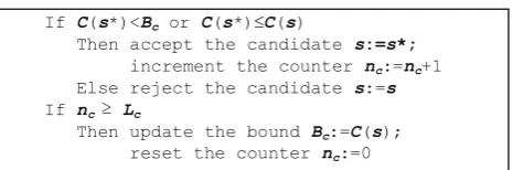
with the cost equal toBcwhen the current cost is also equal toBc, which happens after the update of the cost bound. This is provided by a combination of the SCHC acceptance rule with the greedy rule, i.e. a candidate is also accepted if it is better or equal to the current cost. This enhancement of the acceptance rule provides an extra effectiveness of the search, especially at its final stage where it helps to avoid the effect of “premature convergence”. Thus, at each iteration the SCHC acceptance rule can be expressed by formula (1).

Cs∗<Bc or Cs∗≤C(s) (1)

In this formula,C(s)represents the current cost andC(s∗) the candidate cost, wheres ands* are the current and the candidate solutions, respectively. The complete pseudocode of the initial variant of the SCHC algorithm, which will be called in the rest of this study as “SCHC-all” heuristic is presented in Fig.1.

2.2 Further variants of SCHC

Apart from the basic counting mechanism introduced in the previous section there are many other ways to count the steps during the search. This is a major source of flexibility in the method. For example, we can make it dependent on the qual-ity of candidate solutions. Among possible implementations of this idea, in this study we focus our investigations on three variants of SCHC, which:

1. Counts all moves (SCHC-all).

2. Counts only accepted moves (SCHC-acp). 3. Counts only improving moves (SCHC-imp).

As two additional SCHC heuristics, acp and SCHC-imp, are different from SCHC-all by their counting mech-anisms only, we present the pseudocodes of just these mechanisms. They are depicted in Figs.2and3, which con-tain only the parts different from Fig.1, while the main search

Fig. 1 The pseudocode of SCHC-all heuristic

Fig. 2 The counting/acceptance mechanism of the SCHC-acp heuris-tic

Fig. 3 The counting/acceptance mechanism of SCHC-imp heuristic

loop written in the first eight lines of Fig.1is the same for all variants.

Of course, the variety of potential counting mechanisms is not limited to the ones discussed above. For example, it is possible to develop an intermediate heuristic between SCHC-all and SCHC-acp. This can be done when incrementing the counternc by 1 at all moves and by 2 at accepted moves. Also, we can count unaccepted moves or accepted worsen-ing ones either alone or in any combination. Furthermore, if overlooking the single-parameter conception, we can pro-pose SCHC allowingLcto vary. For example, we can select two different values of the counter limit and interchange them during the search in order to adapt it to some particular search conditions, or we can increaseLcas the run progresses, for example, each time the search goes idle. Along with that, any alternative rule for the variation ofLccould be defined. Interestingly, the SCHC-acp with fixed Lccan be regarded as SCHC-all with variable Lc and vice versa. Finally, the whole counting mechanism can be completely transformed at any point of the search. Thus, the simplicity of the dynamic adjustment of the search process suggests that SCHC can serve as a good platform for experiments with different search patterns, for investigating the search behaviour and for devel-oping self-adaptive heuristics.

3 The experimental environment

3.1 Exam timetabling problem

Generally, these problems contain a high variety of hard and soft constraints. The hard constraints should not be violated in a feasible solution, while the violations of the soft constraints should be minimised. The remaining number of the violations of soft constraints in a solution denotes its quality, measured by a cost function. The most common hard constraint is that no students should sit two exams in the same time. Other hard constraints reflect the limitations on room capacities, the utilisation of specific equipment, pre-defined sequences of exams, etc. The soft constraints represent students, exam-iners and administration preferences, such as time intervals between student’s exams, additional time for marking large exams, etc.

Although the exam timetabling requirements are different in different institutions, in this study we use the specification given in the examination track of the Second International Timetabling Competition ITC2007 (http://www.cs.qub.ac. uk/itc2007/). This site contains a collection of 12 real-world exam timetabling instances, which we use as benchmarks in our experiments with SCHC. Also, this site provides an online validator of the results and a complete description of the hard and soft constraints, which is also published in (McCollum et al. 2010). The characteristics of the instances are presented in Table2in Sect.4.3, in order to facilitate a study into relation between the problem characteristics and the results of our experiments.

3.2 Application details

In this study we adopted software, which was used in experi-ments with LAHC and described in (Burke and Bykov 2012). It is developed in Delphi 2007 and run on PC Intel Core i7-3820 3.6 GHz, 32 GB RAM under OS Windows 7 64 bit.

The search algorithm starts from the generation of a feasi-ble initial solution. The exams are assigned to timeslots using the Saturation Degree graph colouring heuristic. At the same time the exams are randomly assigned to rooms. If the solu-tion is not feasible, then some exams are rescheduled and the initialization procedure starts again. After the generation of the initial solution the heuristic search is run where at each iteration a candidate solution is produced using four types of moves:

• Room movea random exam is moved into a different, randomly chosen room within the same timeslot. • Shift movea random exam is moved into different,

ran-domly chosen timeslot and room. If this move generates an infeasible solution, the algorithm tries to restore the feasibility using the Kempe Chain procedure, which was studied for Graph Colouring Problem byJohnson et al. (1991).

• Swap movethe algorithm selects two random exams and swaps their timeslots. The rooms again are chosen

ran-domly, while the Kempe Chains are used in case of infeasibility.

• Slot move two randomly chosen timeslots are inter-changed including all their exams and rooms.

These four types of moves are selected randomly in equal pro-portions. If the move produces an infeasible candidate, it is just rejected and a new iteration is started. The iteration loop is terminated when no further improvement is possible, i.e. at the convergence state. This state is detected when the number of non-improving (idle) moves since the last improvement reaches at least 1 % of the total number of moves. Also the number of idle moves should be greater than 100 in order to prevent the termination at the beginning. The reason of the use of this stopping condition is discussed in the next section.

4 The investigation into the properties of SCHC

4.1 Cost drop diagrams with differentLc

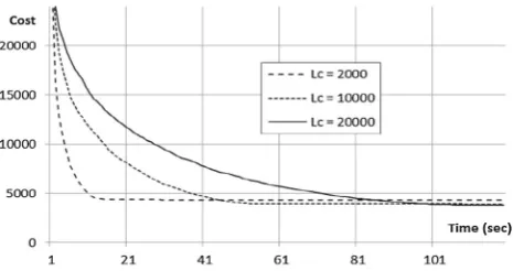
The study of the properties of SCHC starts from the analy-sis of the algorithmic response to the variation of its single parameter. Hence, in our first experiment, we investigate the algorithm’s cost drop diagrams. To produce these diagrams we run each variant of SCHC three times with different val-ues ofLc=2000,10000 and 20000. Each second the current cost was depicted as a point on a plot where the horizontal axis represents the current time and the vertical axis repre-sents the current cost. An example of such a diagram for Exam_1problem produced by SCHC-all heuristic is given in Fig.4. The diagrams produced for other instances by all three studied SCHC heuristics are similar to the presented one. The difference between these diagrams is just in their time and cost scales and that will be discussed in detail in the next section.

The diagram in this figure demonstrates two major prop-erties of SCHC:

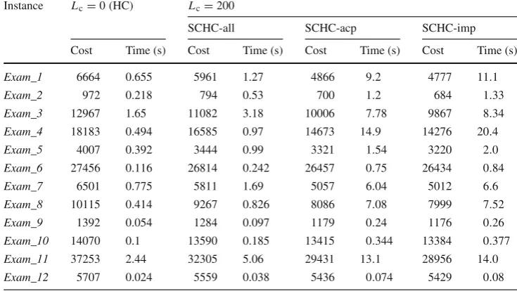
Table 1 The average results of SCHC withLc=0 and

Lc=200

Instance Lc=0(HC) Lc=200

SCHC-all SCHC-acp SCHC-imp

Cost Time (s) Cost Time (s) Cost Time (s) Cost Time (s) Exam_1 6664 0.655 5961 1.27 4866 9.2 4777 11.1 Exam_2 972 0.218 794 0.53 700 1.2 684 1.33 Exam_3 12967 1.65 11082 3.18 10006 7.78 9867 8.34 Exam_4 18183 0.494 16585 0.97 14673 14.9 14276 20.4 Exam_5 4007 0.392 3444 0.99 3321 1.54 3220 2.0 Exam_6 27456 0.116 26814 0.242 26457 0.75 26434 0.84 Exam_7 6501 0.775 5811 1.69 5057 6.04 5012 6.6 Exam_8 10115 0.414 9267 0.826 8086 7.08 7999 7.52 Exam_9 1392 0.054 1284 0.097 1179 0.24 1176 0.26 Exam_10 14070 0.1 13590 0.185 13415 0.344 13384 0.377 Exam_11 37253 2.44 32305 5.06 29431 13.1 28956 14.0 Exam_12 5707 0.024 5559 0.038 5436 0.074 5429 0.08

1. This algorithm converges, i.e. the heuristic search proce-dure lowers the cost until a certain value, after which it does not provide any further improvement. This property is the same as for other local search methods includ-ing HC, SA, LAHC, etc. The presence of this property suggests the use of a common termination condition for such a technique; the search should be stopped exactly at the moment of convergence (the earlier or later termina-tion reduces the effectiveness of the method (seeBurke and Bykov(2012)). The identification of the convergence state can be done by a well-established procedure avail-able in the literature described in the previous section, i.e. when the number of idle moves exceeds a given limit. 2. The variation of Lc affects the convergence time. The

larger the counter limit the slower the current cost drops and it takes longer time to reach the convergence state. Having a search that is automatically terminated at the point of convergence, a user can regulate the total search time by varying Lc. This property has also similarities with other methods. For example, in LAHC the history length also affects the convergence time while in SA the search time can be regulated by the user-defined cooling schedule.

4.2 The comparison of SCHC with hill climbing

An analysis of the second property of SCHC suggests that its search time can be prolonged to any extent with the increase of the counter limit, i.e. the value of Lc has no theoretical upper bound. However, it has the lower bound, which is 0. In this case, the counter is updated at each iteration and all three proposed variants of the method degenerate into greedy Hill Climbing. The same effect will be achieved when assigning

any negative value toLc. This is the fastest variant of SCHC, so the increase of the counter limit does make sense only if this allows to achieve better final results than HC.

To demonstrate that, in the next series of experiments we have applied the discussed above termination rule and run SCHC withLc =0, which is the equivalent to HC, and all three variants withLc=200. Each variant was run on each benchmark instance 50 times. The average results and run times are presented in Table1.

In this table all results produced by either variant of SCHC withLc=200 are better than that of HC, although to a dif-ferent extent. In SCHC-all the search time is approximately twice longer than in HC, which causes a modest improve-ment of the results. However, in SCHC-acp and SCHC-imp the increase of the search time is relatively higher and, cor-respondingly, the improvement of the results is even more distinct.

4.3 The investigation intoLc-diagrams

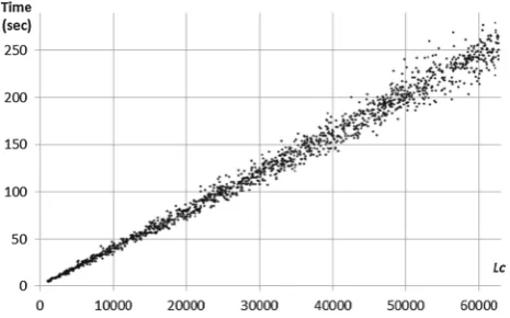
Fig. 5 The dependence of the run time onLcforExam_1dataset with

SCHC-all heuristic

horizontal axis) and the resulting run timeT (in the vertical axis).

Although the points on this diagram are relatively scat-tered, which is typical to any stochastic method, their general distribution forms more or less a straight line. This suggests that the convergence time is approximately proportional to the value of the algorithmic parameterLc. This property of SCHC is similar to the LAHC one studied by Burke and Bykov(2012), where the authors mentioned its high practi-cal importance, i.e. when the angle coefficient (ratioT/Lc) of the distribution is known, the complete search procedure can be fitted into a given available time. The importance of the pre-definition of the search time was underlined in (Burke et al. 2004) especially for long-time searches, which are prac-ticed in pursuit for a higher quality of results.

Our further experiments reveal that the above property is common for SCHC. Although Fig.5presents the linear behaviour of SCHC-all variant applied toExam_1instance, in all other diagrams for three variants of SCHC and 12 benchmark instances the points are also distributed linearly. The diagrams differentiate only by the angles of the produced distributions, i.e. the angle coefficientsT/Lcare highly dif-ferent for difdif-ferent instances and variants of SCHC. However, our preliminary observations have revealed certain tenden-cies in the values of these coefficients. In particular, the highest values are typical for SCHC-imp, slightly lower for SCHC-acp and much lower for SCHC-all heuristics. Consid-ering a single variant of SCHC, a certain dependency of the coefficients on the size of a dataset can be also noticed. The general tendency is the following: the larger the instance, the larger the angle coefficient. The coefficients together with the main characteristic of our benchmark instances sorted by the number of exams are shown in Table2.

In this table, the proposed tendency of the dependence of T/Lcon the instance size can be observed for the majority of problems. However, there are a number of exceptions to this rule. For example, the coefficients forExam_2instance are

much smaller than for the other problems of the same or even lower size. Another anomaly is in Exam_4 problem. This dataset has only one room, so the “room moves” described in Sect.3.2are not applicable here. De facto, we are dealing here with a different problem formulation. The oddity of this problem is also seen in its coefficients. The coefficient for SCHC-all fits into the above tendency, but coefficients for both SCHC-acp and SCHC-imp are much higher than can be expected for a problem of this size. In addition,Exam_3 and Exam_11 instances represent the same dataset where Exam_11is just a more constrained variant, i.e. it should be scheduled into a less number of timeslots and rooms. Cor-respondingly, we see the different values of T/Lc for these problems in Table2.

This tendency was also observed in LAHC by (Burke and Bykov 2012), who proposed that some other factors, together with the size of problems, could also affect the values of the angle coefficients, such as constraints, conflict density, etc. If assuming that the amount of these factors somehow defines thehardnessof a problem, then the angle coefficient might reflect, to some extent, this “bulk” hardness. The investiga-tion into the hardness of different problems represents an important area of combinatorial optimisation studies. There are a number of theoretical publications, where the authors investigate the hardness based on the analysis of problem characteristics, for example (Smith-Miles and Lopes 2012). However, the idea proposed here suggests an alternative way, i.e. to use aheuristic measureof the hardness of different problems. This means that a heuristic algorithm can serve not just for solving a problem, but also as a tool for measur-ing its hardness.

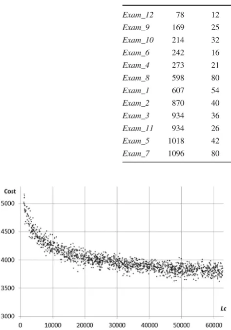
To advocate the importance of the investigations into the hardness of optimisation problems, we analyseLc-cost dia-grams of the datasets. These diadia-grams are plotted using the previous experimental data, which were already used in the diagram in Fig.5, but now the diagrams show the dependence of the final cost on the specified Lc. The example of such a diagram for SCHC-all heuristic applied toExam_1problem is shown in Fig.6. Here, once again, the result of each run is depicted as a point, whose horizontal coordinate represents Lcand the vertical coordinate represents the final cost.

This diagram demonstrates a clear dependence of the final cost on Lcand correspondingly on the total run time as the time is linearly dependent on Lc, i.e. the larger the counter limit (the longer the search)—the better the result. For exam-ple, despite the scatter, any, even the worst one, result with Lc=50000 isguaranteed betterthan any of the results with Lc=5000. Obviously, this diagram confirms the opinion of Johnson et al. (1989) for SA that “up to a certain point, it seems to be better to perform one long run than to take the best of a time-equivalent collection of shorter runs”.

Table 2 The characteristics of the ITC2007 instances and their T/Lccoefficients

Instance Number of exams

Number of timeslots

Number of rooms

Density CoefficientT/Lc

×10−3

SCHC-all SCHC-acp SCHC-imp Exam_12 78 12 50 0.18 0.105 0.23 0.28 Exam_9 169 25 3 0.078 0.26 0.99 1.12 Exam_10 214 32 48 0.05 0.47 1.17 1.35

Exam_6 242 16 8 0.062 0.64 3.4 3.8

Exam_4 273 21 1 0.15 1.72 56 73

Exam_8 598 80 8 0.046 3.1 36 42

Exam_1 607 54 7 0.5 4.2 59 65

Exam_2 870 40 49 0.012 1.94 4.8 5.5

Exam_3 934 36 48 0.026 8.7 29 31

Exam_11 934 26 40 0.026 12.8 47 53

Exam_5 1018 42 3 0.0087 3.5 7.1 7.6

Exam_7 1096 80 15 0.019 6.3 28 33

Fig. 6 The dependence of the final cost onLcforExam_1problem

with SCHC-all heuristic

be more effective to produce a number of short runs while employing various “multi-start” or “reheating” strategies and then to pick up the best result. For example,Boese et al. (1994) indicated that “several studies have shown greedy multi-start superior to simulated annealing in terms of both solution quality and run time”.

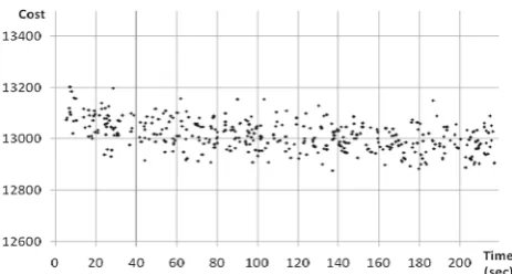
Having two so contrasting opinions from the trusted sources we can assume that the origin of such a dilemma is in the diversity of the studied problems. For example, in our exam timetabling collection the shape ofLc-cost diagrams is not the same for all benchmark datasets in contrast to theL c-time diagrams, which are quite similar. As an illustration, Fig.7 depicts the Lc-cost diagram for Exam_10 problem, whose shape is quite different from Fig.6.

Except for the very small values ofLc, this diagram does not expose a sensible dependence of the final cost on the value of the counter limit, i.e. the average and the best costs are almost the same either with smaller Lc or with larger Lc, although the latter causes a longer search time. In this

Fig. 7 The dependence of the final cost onLcforExam_10problem

with SCHC-all heuristic

situation, a more effective strategy is to produce multiple short runs and pick up the best result among them.

However, the idea of the selection of the best search strat-egy by plotting theLc-cost diagrams has no practical value. First, this diagram can be obtained only after running the algorithm a large number of times, which incurs huge com-putational expenses (in our experiments it took around 4 days of continuous runs for each diagram). Second, after all these runs the problem is already solved and the best search strat-egy is identified just post-factum.

groups. Diagrams, which follow the pattern shown in Fig.6, are characteristic to 6 out of 12 datasets:Exam_1,Exam_3, Exam_5,Exam_7,Exam_8andExam_11. For the remaining 6 datasets:Exam_2,Exam_4,Exam_6,Exam_9,Exam_10 andExam_12the shapes are close to the one given in Fig.7. When comparing these two groups with Table 2, we can observe quite a strong correlation between the shape of the diagram and the value ofT/Lc. The problems with the larger values ofT/Lc(harder ones) have more distinct dependence of cost onLc, i.e. the shapes are close to Fig.6, while the diagrams with the shape shown in Fig.7 are more typical to the problems with the smaller values ofT/Lc, which are presumably less hard ones. It seems that the revealed con-nection between the shape of theLc-cost diagram and the T/Lccoefficient is stronger than the connection between the shape of the diagram and the size of a problem.

Although this study presents experiments with 12 instances and three SCHC heuristics only, the results have demonstrated that for at least these datasets we can already skip the awkward diagram building stage and identify the best search strategy based just on the value ofT/Lc, which is obtainable by a single short-time run, i.e. if this value is relatively low, then a multi-start approach is preferred. Other-wise, if this value is relatively high, a single long run will be more effective. Of course, the justification of this hypothesis and its practical implementation require much more exten-sive study on a larger number of benchmark problems and with other SCHC heuristics. However, our preliminary tests with the travelling salesman and grid scheduling problems have revealed the same algorithmic behaviour. Therefore, we believe that this represents a very promising direction of a future research.

4.4 Cost drop diagrams of different variants of SCHC

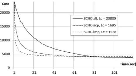
The question about the choice of the best search strategy is not limited to the above example. The investigations in this field are especially relevant to SCHC, which supposes a large number of variants and extensions where it is necessary to make a choice between them. In this situation, it is important to estimate the difference in the search behaviour between different heuristics. Hence, the following series of experi-ments are designed to analyse search strategies employed by our three variants of SCHC. Similar to the first experiment we do that by plotting their cost drop diagrams. Moreover, taking into consideration theT/Lccoefficients we can now tune our SCHC heuristics in order to provide the same con-vergence time for each of the variants. The value ofLccan be calculated by dividing the required time by theT/Lc coeffi-cient from Table2. In our test, the three heuristics were run withExam_1dataset for 100 s, hence the calculated values ofLcwere: all: 23800, acp: 1695 and

SCHC-Fig. 8 The cost drop diagrams of different SCHC heuristics with Exam_1instance

imp: 1538. The resulting cost drop diagrams are presented in Fig.8.

The analysis of these diagrams gives an idea about the difference in search strategies between these heuristics. SCHC-imp jumps quickly into the region of low-cost solu-tions and then spends the most of the search time in this region while slowly improving the quality of result. The SCHC-acp heuristic does the same, but slightly smoother; it goes into the region of low-cost solutions more slowly and spends less time staying there. In contrast, the SCHC-all heuristic pays much more attention to exploring the high-cost solutions. It spends in that region about a half of the search time while the time spent for the final improvement is much shorter.

The convergence time in these diagrams is the same for each heuristic so the quality of a final result might be dependent on how the particular search strategy fits into the problem’s landscape. Our experiments presented in the next section show that there is no general preference to any of the heuristics. Their performance is highly problem-dependent and different problems acquire different best performed strategies. However, together with the shapes of the diagrams some other internal properties of these variants could affect their performance on different instances. This issue warrants a further investigation.

5 A comparison of SCHC with other methods

The developed variants of SCHC were compared with SA, GD and LAHC algorithms. Firstly, we test the performance of these methods on original ITC2007 problems. Secondly, we test the reliability of these methods using an artificially created non-linear optimisation problem.

5.1 A performance test

problems there could be an evident dependence of the quality of results on the total search time. Moreover, the final results produced by SCHC even in the same CPU time are scattered within certain cost interval. Obviously a good comparison method should take into consideration such a behaviour of SCHC as well as the behaviour of the other methods.

To investigate that, we repeated the experiment described in Sect.4.3with the methods selected for the comparison, i.e. we run them many times (around 500) while randomly varying their time-related parameters: cooling factor in SA, decay rate in GDA and history length in LAHC. The random variation of the parameters was organised in such a way, that we got uniform time-cost diagrams similar to the ones presented in Figs.6and7. An interested reader can found these diagrams for all benchmark datasets produced by SA together with the ones for SCHC in the journal online supple-ment. A visual comparison of these diagrams indicates that for each dataset the diagram shapes of SA and SCHC are quite similar, which implies the similar behaviour of these methods. The same is also relevant to GDA and LAHC. As an illustration, the time-cost diagrams produced by SA forExam_1andExam_10problems are presented in Figs.9 and10. When comparing them with Figs.6and7, respec-tively, we can see that for the same instances the shapes of the diagrams are very similar even being produced by different methods.

Fig. 9 The time-cost diagram produced by SA forExam_1problem

Fig. 10 The time-cost diagram produced by SA forExam_10problem

When different algorithms show similar behaviour in respect of computing time, the differences between them should be evaluated to make conclusions about their perfor-mance. To rely only on the visual comparison of noisy curves is not satisfactory, so in order to get a more detailed infor-mation we apply a “cut-off” approach proposed in (Burke and Bykov 2012). To explain this method, we divided the diagrams in Figs.9 and10by vertical gridlines into equal segments of 20 s length, which gives in total 10 segments. When observing these segments separately, the distribution of points within each of them gives an idea about the perfor-mance of the method being run within the corresponding time boundaries. For example, the points in segment (160,180) in Fig.9 show that SA being run onExam_1problem for 160–180 s is able to achieve final cost values approximately between 3850 and 4150, which is on average 4000. The cut-off approach employs a usual evaluation of average costs but takes into account the computing time. In this method, the average performance of an algorithm is represented by a set of average values calculated for all segments. This enables the sets produced by different methods to be compared in a table.

In our experiments, we have produced the cut-off sets for SA, GDA, LAHC and the three studied variants of SCHC for all our benchmark instances. To ensure the adequate perfor-mance of SA, we use general suggestions from the literature for its parameterization. We employ a geometric cooling schedule while the initial temperature is set up in such a way so that in the initial phase of the search the algorithm accepts 85 % of non-improving moves. In contrast, GDA, LAHC and SCHC do not require any special initialization procedure. Table3presents the resulting cut-offs forExam_1dataset, where the best results over six heuristics are highlighted in bold.

This table demonstrates the clear superiority of two vari-ants of SCHC (acp and imp) over the other methods on runs longer than 20 s. On shorter runs LAHC performs better, but both LAHC and SCHC-all slightly underperform on the longer runs. Nevertheless, SA performs much inferior to both LAHC and all variants of SCHC on the runs of any length. Finally, GDA has the worst performance than any other method.

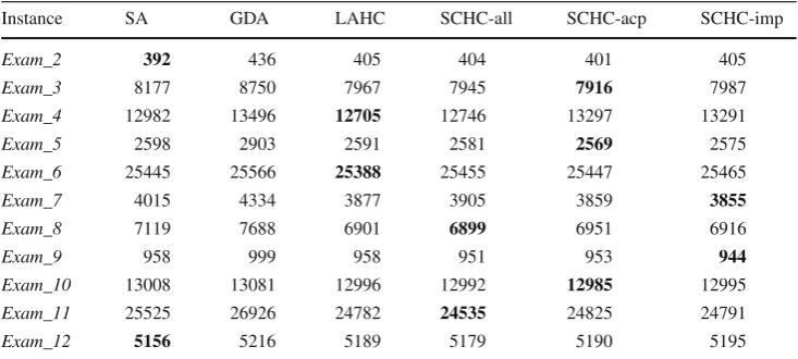
We produced the same tables for all benchmark instances, which show quite problem-dependent performance of dif-ferent methods. They are not included in the paper, but are available in the online supplement. To give an idea about this performance, in Table4, a compilation of the collection of cut-offs for all datasets for the middle interval of 100–120 s is presented.

Table 3 The cut-offs for SA, GDA, LAHC and SCHC (all, acp, imp) forExam_1dataset

CPU time (s) SA GDA LAHC SCHC-all SCHC-acp SCHC-imp

0–20 4879 5224 4640 4646 4656 4711

20–40 4513 4804 4305 4330 4276 4286

40–60 4342 4593 4190 4150 4147 4129

60–80 4228 4496 4084 4061 4066 4053

80–100 4175 4439 4029 4029 4007 3985

100–120 4109 4358 3986 3978 3927 3952

120–140 4087 4335 3939 3924 3906 3900

140–160 4041 4300 3912 3890 3872 3863

160–180 3982 4251 3899 3869 3851 3859

180–200 3996 4213 3864 3852 3809 3819

Table 4 The cut-offs for SA, LAHC and SCHC (all, acp, imp) for other ITC2007 datasets

Instance SA GDA LAHC SCHC-all SCHC-acp SCHC-imp

Exam_2 392 436 405 404 401 405

Exam_3 8177 8750 7967 7945 7916 7987

Exam_4 12982 13496 12705 12746 13297 13291

Exam_5 2598 2903 2591 2581 2569 2575

Exam_6 25445 25566 25388 25455 25447 25465

Exam_7 4015 4334 3877 3905 3859 3855

Exam_8 7119 7688 6901 6899 6951 6916

Exam_9 958 999 958 951 953 944

Exam_10 13008 13081 12996 12992 12985 12995 Exam_11 25525 26926 24782 24535 24825 24791

Exam_12 5156 5216 5189 5179 5190 5195

is considerably weaker, namely on 8 problems its results are worse than results of either LAHC or SCHC and only on two instances SA performs the best. Once again, GDA has the worst performance over six methods.

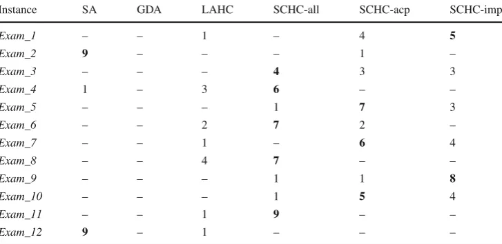
To further study the general tendencies in the performance of the compared methods on different datasets, we present another compilation of the cut-off results for all instances. For each instance we count the number of segments over the whole time interval where each method performs the best. Table5presents such numbers for all 12 datasets, where the largest numbers of the “winning” segments are highlighted by bold.

The analysis of this table confirms a distinctive good per-formance of SA on Exam_2 and Exam_12 problems. In both cases it wins in 9 over 10 time segments. For other 10 problems, different variants of SCHC perform the best across segments. For example, SCHC-all has a distinctive performance onExam_6,Exam_8andExam_11problems, SCHC-imp has a distinctive performance onExam_9, while SCHC-acp and SCHC-imp both have a good performance on Exam_1, Exam_7 andExam_10 problems. Finally, on Exam_3all three variants of SCHC have approximately the same performance.

In our analysis, of a particular interest is the comparison of the results given in Tables4and5with the values ofT/Lcin Table2, which seems to reflect the problem hardness. First, SCHC wins on all six relatively harder problems. Second, SA shows a good performance just on datasets that are to some extent uncommon. For example,Exam_12is exceptionally small problem;Exam_2problem has disproportionally low values ofT/Lc(see Sect.4.3). The oddity ofExam_4 prob-lem was also discussed previously. It could happen that the performance of SCHC with the single-room problem is more dependent on the shape of cost drop diagram (see Fig.8) than with other ones.

5.2 A reliability test

Table 5 The numbers of winning segments of SA, LAHC and SCHC (all, acp, imp) for all datasets

Instance SA GDA LAHC SCHC-all SCHC-acp SCHC-imp

Exam_1 – – 1 – 4 5

Exam_2 9 – – – 1 –

Exam_3 – – – 4 3 3

Exam_4 1 – 3 6 – –

Exam_5 – – – 1 7 3

Exam_6 – – 2 7 2 –

Exam_7 – – 1 – 6 4

Exam_8 – – 4 7 – –

Exam_9 – – – 1 1 8

Exam_10 – – – 1 5 4

Exam_11 – – 1 9 – –

Exam_12 9 – 1 – – –

dataset was used with transformation (2) applied to its cost function. Thus, in the new problem, the cost functionCresis represented as a cubical polynomial of the original costC.

Cres=C3−48000×C2+770×106×C (2)

Expression (2) represents a monotonically increasing func-tion because its first derivative is a quadratic polynomial with a positive first coefficient and a negative discriminant, and therefore, this derivative is always positive. Hence, all original local and global optima are preserved in the new problem, i.e. when solution A has a higher cost than solution B in the original problem, it holds true in the new prob-lem also. The new and the original probprob-lems are the same from the point of view of dominance relations between solu-tions, while the rescaling differentiates only the distances between solutions (usually called as “delta costs”). Conse-quently, rescaling expressed by (2) affects the performance of algorithms which evaluate delta costs, such algorithms are SA or GDA. However, it has no effect on algorithms which employ the ranking of solutions such as HC or LAHC. With the same initial randomization, the search paths of these

algo-rithms is the same for the original and the rescaled problems and they will achieve the same final results. The proposed SCHC is also based on the solution ranking and does not evaluate delta costs (see pseudocodes in Figs.1,2,3), there-fore a monotonic rescaling of the cost function should not affect the performance of the algorithm.

To verify empirically this proposition, we run the same experiment as in Sect.5.1on the rescaled problem. Apart from the new problem formulation, all other experimental conditions remain the same as explained. Only the initial temperature of SA was tuned again in order to comply with the literature suggestion that there is 85 % of non-improving moves at the beginning. The results of this test are shown in Table6. To simplify an assessment of these results, we present in this table their non-rescaled values.

The results confirm that the rescaling given by (2) con-siderably deteriorates the performance of SA and to the less extent GDA but does not affect any studied variant of SCHC in the same way as LAHC. This example supports a contention that SCHC is more reliable than SA. In this experiment, we resort to a highly non-linear artificial prob-lem specially designed for the purpose of enhancing the effect

Table 6 The cut-offs for SA, GDA, LAHC and SCHC (all, acp, imp) forExam_1dataset with the rescaled cost function

CPU time (s) SA GDA LAHC SCHC-all SCHC-acp SCHC-imp

0–20 5487 5526 4636 4671 4657 4663

20–40 5227 5089 4307 4322 4277 4285

40–60 5091 4893 4152 4138 4116 4096

60–80 5013 4792 4073 4071 4029 4033

80–100 4977 4773 4003 4027 3958 3943

100–120 4929 4710 3953 3973 3922 3934

120–140 4907 4604 3921 3910 3885 3892

140–160 4892 4574 3891 3875 3862 3858

160–180 4852 4495 3854 3864 3828 3839

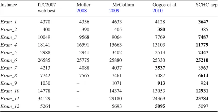
Table 7 The comparison of our best results with ITC2007 and post-competition ones

Instance ITC2007 web best

Muller 2008

McCollum 2009

Gogos et al. 2010

SCHC-acp

Exam_1 4370 4356 4633 4128 3647

Exam_2 400 390 405 380 385

Exam_3 10049 9568 9064 7769 7487

Exam_4 18141 16591 15663 13103 11779

Exam_5 2988 2941 3402 2513 2447

Exam_6 26585 25775 25880 25330 25210

Exam_7 4213 4088 4037 3537 3563

Exam_8 7742 7565 7461 7087 6614

Exam_9 1030 – 1071 913 924

Exam_10 14778 – 14374 13053 12931

Exam_11 34129 – 29180 24369 23784

Exam_12 5264 – 5693 5095 5097

of the non-linearity on the search process. However, when the non-linearity of a problem is not so distinct, the deterioration of the SA performance might be less clear, although it is still present. If we assume that the presence of a high number of hard constraints, which exclude infeasible solutions from the search space, somehow provides a non-linear effect, then this could explain the underperformance of SA also on the original problems.

6 Comparison with published results

To complete the evaluation of SCHC performance, we com-pare its results with the actual best ITC2007 results and with the results presented in pre-competition (Muller 2008) and post-competition publications:McCollum et al.(2009) and Gogos et al.(2010). In this series of experiments, we respect the ITC2007 restrictions on the maximum run time and the number of independent runs. The maximum run time was calculated using the ITC2007 benchmarking application; for our experimental PC it was 204 s. Also, the best result was selected over 10 independent runs on each benchmark prob-lem. Our best results together with the published ones are presented in Table7where the best results are highlighted in bold. All our best results are verified using the online valida-tor provided by ITC2007 organisers.

In this comparison, we use SCHC-acp variant because in our previous experiments it has shown the strongest per-formance (see Table4). To provide the convergence of the algorithm exactly in the given time, the value ofLcwas cal-culated for each instance based on the values ofT/Lcfrom Table2. In such a way we employ some beforehand collected information about the algorithmic behaviour on benchmark instances and therefore we do not claim that this series of experiments mimics our participation in the competition. The most of the post-competition studies do not pursue that

goal either which is in line with the discussion byMcCollum et al.(2009) that adherence to the competition rules in any post-competition publication is rather artificial because many additional factors should be taken into account. The results of Gogos et al.(2010) can be considered as the best up to date; however, the authors indicated that they were produced “under no hardware or time limit”, i.e. without following ITC2007 rules at all. Hence, in this comparison, we have an advantageous position over the actual ITC2007 results, the same position withMuller(2008) andMcCollum et al.(2009) but the position ofGogos et al.(2010) is more advantageous than ours.

This table once again demonstrates the strong perfor-mance of our proposed method. For eight benchmark problems SCHC has achieved results better than the best previously published ones. Although for four remaining problems our results are inferior toGogos et al.(2010), they are still very competitive. It is interesting to observe that Exam_2andExam_12are among the instances on which the method byGogos et al.(2010) performed better, which com-plies with the discussions provided in the previous sections.

7 Conclusions

In this study, we proposed a new local search algorithm: SCHC and investigated its behaviour. The exam timetabling problem was chosen as benchmark. Our experiments have revealed that SCHC shares a number of properties with LAHC:

• SCHC has a strong performance on the benchmark prob-lems.

• The search time is approximately proportional toLcand the coefficient of proportionality is usually larger for the problems, which seemed to be harder.

• SCHC does not employ any type of cooling schedule. • SCHC is more reliable than cooling schedule based

meth-ods (e.g. SA), i.e. it works well on specific problems where SA fails to produce good results.

However, SCHC has several additional distinct properties:

• The counting mechanism can be implemented in a variety of ways. So, for each particular problem we can find the most suitable variant of SCHC.

• The counting mechanism in SCHC is very flexible. Dur-ing the search, the value of the counter limit can be easily adjusted at any iteration to respond to the obtained results. Moreover, the whole counting mechanism can be changed throughout the search. Therefore, SCHC can serve as a good platform for developing various self-adaptive methods.

• SCHC is a very simple and transparent method, easy to understand and implement. Hence, it has a high potential in the education area. By studying SCHC as a first meta-heuristic, the students could quicker get into the ABC’s of search methodologies. For this purpose, we have included SCHC into our “Multi-Heuristic Solver” software appli-cation, which is available for download fromhttp://www. yuribykov.com/MHsolver/.

The main emphasis of this paper is on the investigation into the behaviour of the proposed algorithm. Some observed dependencies in this behaviour motivated the hypothesis that in addition to the solving optimisation problems SCHC can be also used as a tool for heuristic measuring their hardness. We have proposed that the research into the hardness of differ-ent problems might help to iddiffer-entify an optimal search strategy for a particular dataset. The results of our experiments pro-vide some empirical support for our ideas. However, the justification of these hypotheses requires further and much wider investigations with different problems and variants of SCHC. Apart from that, the research into the further prop-erties of SCHC, its behaviour with different problems and the modifications of this method (especially the self-adaptive ones) as well, as its practical and educational applications is also seen as a quite interesting subject of a future work.

Acknowledgments The work described in this paper was carried out under a Grant (EP/F033214/1) awarded by the UK Engineering and Physical Sciences Research Council (EPSRC).

Open Access This article is distributed under the terms of the Creative Commons Attribution 4.0 International License (http://creativecomm ons.org/licenses/by/4.0/), which permits unrestricted use, distribution, and reproduction in any medium, provided you give appropriate credit

to the original author(s) and the source, provide a link to the Creative Commons license, and indicate if changes were made.

References

Abdullah, S., & Alzaqebah, M. (2014). An adaptive artificial bee colony and late acceptance hill-climbing algorithm for examina-tion timetabling.Journal of Scheduling,17, 249–262.

Abuhamdah, A. (2010). Experimental result of late acceptance random-ized descent algorithm for solving course timetabling problems. International Journal of Computer Science and Network Security, 10, 192–200.

Boese, K. D., Kahng, A. B., & Muddu, S. (1994). A new adaptive multi-start technique for combinatorial global optimizations.Operations Research Letters,16, 101–113.

Burke E. K., & Bykov, Y. (2008). A late acceptance strategy in hill-climbing for exam timetabling problems:Proceedings of the 7th International Conference on the Practice and Theory of Automated Timetabling (PATAT2008), Montreal, Canada.

Burke E. K., & Bykov, Y. (2012). The Late Acceptance Hill Climb-ing heuristic. Technical report CSM-192, ComputClimb-ing Science and Mathematics, University of Stirling, UK.

Burke, E. K., Bykov, Y., Newall, J., & Petrovic, S. (2004). A time-predefined local search approach to exam timetabling problems. IIE Transactions,36(6), 509–528.

Burke, E. K., McColumn, B., Meisels, A., Petrovic, S., & Qu, R. (2007). A graph-based hyper-heuristic for educational timetabling prob-lems.European Journal of Operational Research,176, 177–192. Burke, E. K., & Petrovic, S. (2002). Recent research directions in auto-mated timetabling.European Journal of Operational Research, 140, 266–280.

Bykov Y., & Petrovic, S. (2013). An initial study of a novel Step Counting Hill Climbing heuristic applied to timetabling problems: Proceedings of 6th Multidisciplinary International Scheduling Conference (MISTA 2013), Gent, Belgium.

Carter, M. W., Laporte, G., & Lee, S. (1996). Examination timetabling: algorithmic strategies and applications.Journal of the Operational Research Society,47, 373–383.

Di Gaspero, L., & Schaerf, A. (2001). Tabu search techniques for exami-nation timetabling.Practice and Theory of Automated Timetabling III, Lecture Notes in Computer Science. Berlin: Springer. Erben, W. (2001). A grouping genetic algorithm for graph colouring and

exam timetabling.Practice and Theory of Automated Timetabling III, Lecture Notes in Computer Science. Berlin: Springer. Goerler, A., Schulte, F., & Voss, S. (2013). An application of late

acceptance hill climbing to the traveling purchaser problem. Com-putational logistics, Lecture Notes in Computer Science. Berlin: Springer.

Gogos, C., Goulas, G., Alefragis, P., Kolonias, V., & Housos, E. (2010). Distributed Scatter Search for the examination timetabling prob-lem.PATAT 2010 Proceedings of the 8th International Conference on the Practice and Theory of Automated Timetabling, Belfast, UK. Jackson W., Özcan, E., & Drake, J. H. (2013). Late acceptance-based selection hyper-heuristics for cross-domain heuristic search.The 13th UK Workshop on Computational Intelligence, Guildford, UK. Johnson, D. S., Aragon, C. R., McGeoch, L. A., & Schevon, C. (1989). Optimization by simulated annealing: an experimental evaluation. Part II, graph partitioning.Operations Research,37(3), 865–892. Johnson, D. S., Aragon, C. R., McGeoch, L. A., & Schevon, C. (1991). Optimization by simulated annealing: an experimental evalua-tion; Part II, graph coloring and number partitioning.Operations Research,39(3), 378–406.

examina-tion timetabling problem:Proceedings of the 4th Multidisciplinary International Conference on Scheduling: Theory and Applications (MISTA09), Dublin, Ireland, 424–434.

McCollum, B., Schaerf, A., Paechter, B., McMullan, P. J., Lewis, R., Parkes, A. J., et al. (2010). Setting the research agenda in automated timetabling: The second international timetabling competition. INFORMS Journal on Computing,22, 120–130.

Merlot, L., Boland, N., Hughes, B., & Stuckey, P. (2003). A hybrid algorithm for the examination timetabling problem. Practice and Theory of Automated Timetabling IV.Lecture Notes in Computer Science, Berlin: Springer

Muller, T. (2008). ITC2007 solver description: a hybrid approach. Proceedings of the 7th International Conference on the Practice and Theory of Automated Timetabling (PATAT 2008), Montreal, Canada.

Özcan, E., Bykov, Y., Birben, M., & Burke, E. K. (2009). Examination timetabling using late acceptance hyper-heuristics:Proceedings of the 2009 IEEE Congress on Evolutionary Computation (CEC’09), Trondheim, Norway.

Petrovic, S., & Bykov, Y. (2003). A multiobjective optimisation tech-nique for exam timetabling based on trajectories.Practice and Theory of Automated Timetabling IV, Lecture Notes in Computer Science. Berlin: Springer.

Petrovic, S., Patel, V., & Young, Y. (2005). University timetabling with fuzzy constraints.Practice and Theory of Automated Timetabling V, Lecture Notes in Computer Science. Berlin: Springer. Qu, R., Burke, E. K., McCollum, B., Merlot, L. T. G., & Lee, S. Y.

(2009). A survey of search methodologies and automated system development for examination timetabling.Journal of Scheduling, 12, 55–89.

Schaerf, A. (1999). A survey of automated timetabling.Artificial Intel-ligence Review,13, 87–127.

Smith-Miles, K., & Lopes, L. (2012). Measuring instance difficulty for combinatorial optimization problems.Computers and Operations Research, 39, 875–889.

Swan, J., Drake, J., Ozcan, E., Goulding, J., & Woodward, J. (2013). A comparison of acceptance criteria for the Daily Car-Pooling problem.Computer and Information Sciences,III, 477–483. Thompson, J. M., & Dowsland, K. A. (1996). Variants of simulated

annealing for the examination timetabling problem.Annals of Operations Research,63, 105–128.

Tierney, K. (2013). Late acceptance hill climbing for the liner shipping fleet repositioning.Proceedings of the 14th EU/ME Workshop, 21– 27.

Verstichel, J., & Vanden Berghe, G. (2009). A late acceptance algorithm for the lock scheduling problem.Logistic Management,2009(5), 457–478.

Vancroonenburg, W., & Wauters, T. (2013) Extending the late accep-tance metaheuristic for multi-objective optimization.Proceedings of the 6th Multidisciplinary International Scheduling conference: Theory & Applications (MISTA2013). Ghent, Belgium.