Wave steering effects in anisotropic composite structures: direct calculation of the energy skew angle through a finite element scheme

Wave steering e

ff

ects in anisotropic composite structures: Direct calculation of

the energy skew angle through a finite element scheme

D. Chronopoulosa

a_{Institute for Aerospace Technology & The Composites Group, The University of Nottingham, NG7 2RD, UK}

Abstract

A systematic expression quantifying the wave energy skewing phenomenon as a function of the mechanical charac-teristics of a non-isotropic structure is derived in this study. A structure of arbitrary anisotropy, layering and geomet-ric complexity is modelled through Finite Elements (FEs) coupled to a periodic structure wave scheme. A genegeomet-ric approach for efficiently computing the angular sensitivity of the wave slowness for each wave type, direction and fre-quency is presented. The approach does not involve any finite differentiation scheme and is therefore computationally efficient and not prone to the associated numerical errors.

Keywords: Wave Steering, Composite Structures, Energy skewing, Caustics, Wave Finite Elements

1. Introduction

Understanding complex wave phenomena is of paramount importance for the successful application of ultrasonic techniques within the non-destructive testing (NDT) and biomedical fields. Accurate and efficient modelling of elas-tic wave propagation complex phenomena in composite structures play a crucial role in the development of robust algorithms for damage detection and localization. One of the most prominent of these phenomena is the so-called en-ergy skewing (see Fig.1), induced by the angular divergence between the phase and group velocities for non-isotropic configurations. Wave skewing results in a non-uniform distribution of energy along the wavefront. An inaccurate description of the skewing effect in the computational models and NDT algorithms can well result in an incorrect prediction of damage location [1, 2] and type.

Directional dependence of the wave slowness characteristics in non-isotropic structures has been well discussed and investigated by several researchers. In [3] the authors demonstrated a material anisotropy-based, beam-steering scheme for electronically steering an acoustic beam over an angle larger than 70o _{in a TeO}

2 crystal. The idea was based on the pronounced angular dependency of the wave skewing angle in the same material. Wave beam steering through the employment of phased array transducers [4] has been discussed within the context of several applications including biomedical imaging [5], structural health monitoring [6, 7, 8] and acoustic applications [9]. With regard to layered cellular composites, the researchers in [10, 11, 12] derived wave propagation models based on Bloch’s

theorem in order to show how band-gaps and strong acoustic focusing can be affected by structural anisotropy in periodic lattice structures.

Calculation of the wavefront curve has formed the basis for most researchers in order to quantify wave steering effects. The wave skewing angle has been calculated by a number of authors through a variety of approaches, including the application of a Fresnel approximation to the wave propagation problem [13], derivation through the propagating group velocities in two orthogonal directions within the panel [14], as well as through a Finite Differentiation (FD) approach [15]. To the best of the author’s knowledge, there is currently no expression directly quantifying the wave skewing effect as a function of the mechanical characteristics of the non-isotropic structure.

The principal objective and contributing novelty of this study is the derivation of a systematic and robust expression relating the wave energy skew angle to the material characteristics of the composite structure under investigation. A robust FE-based approach for efficiently computing the angular sensitivity of the wave phase velocities for each wave type, direction and frequency is presented. The considered structure can be of arbitrary layering and material characteristics as FE modelling is employed. The exhibited scheme is able to compute the wavenumber angular sensitivity (and subsequently the energy skew angle) by determining and post-processing a single solution of the system. This overcomes the drawbacks of the currently employed FD approaches.

The paper is organized as follows: In Sec.2 a general expression is derived for the angle of the propagating energy wavefront as well as the skew angle between the phase and group velocities for each wave type as a function of the wavenumber angular sensitivity. In Sec.3 a direct expression of the wavenumber sensitivity with respect to the direction of propagation is derived within a FE modelling context. Numerical case studies validating the computational scheme are presented in Sec.4. Conclusions on the exhibited work are eventually drawn in Sec.5.

2. Calculation of the wave energy skew angle

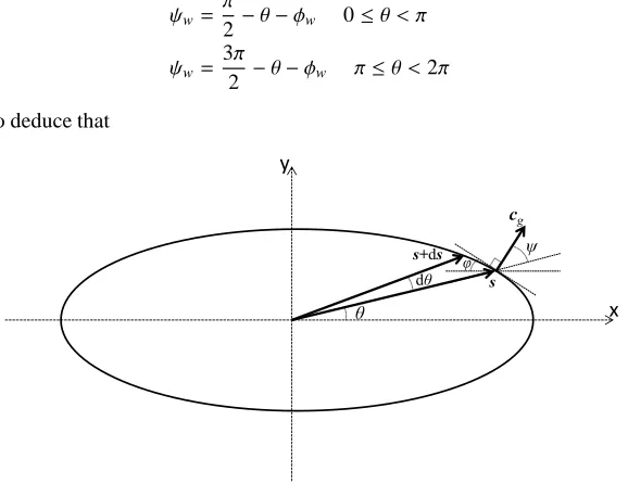
Slowness curves are particularly useful for visualizing the direction of the group velocity (see Fig.1). On the other hand, the velocity of the wavefront (defined as the locus of ray velocity vectors along all directions starting from the origin) in the direction normal to the wavefront is known as the phase velocity. In an anisotropic material, the phase and group velocities are generally different [16] and a clear distinction between the two should be made to ensure that the correct velocity profile is employed when performing health monitoring with an ultrasonic device. The physical difference between the phase and group velocities can be described by considering a propagating wave packet (see Fig.1). The wavefronts remain normal to the the phase velocity directionθ(or equivalently, parallel to the transducer surface exciting the packet), however due to material anisotropy the wave packet skews away from the normal direction by an angleψ and instead travels along a shifted ray path. The velocity of the wave packet envelope is given by the group velocity cg. It has been well documented [14] that the group velocity vector is always

perpendicular to the tangent of the slowness curve. Moreover, it is reminded that the slowness of a wave w can be expressed as sw=

kw

ωw

When the angular rate of change for each propagating wavenumber kwis known (see Sec.3), the skew angleψw

can be determined through geometric considerations. In Fig.1, a representation of an infinitesimal change of angle dθand correspondingly of slowness dsw is drawn. In the same figure the angle of the tangent to the slowness with

respect to the horizontalφis shown. As vector cgis perpendicular to the drawn tangent and swforms an angleθto the

horizontal, the skew angleψwcan be determined as

ψw=

π

2 −θ−φw 0≤θ < π

ψw=

3π

2 −θ−φw π≤θ <2π

(1a)

(1b)

It is straightforward to deduce that

x y

s+ds

s

dθ

θ

φ ψ

c

g

Figure 1: Illustration of the group velocity being perpendicular to the wave slowness curve for a non-isotropic structure. A wave energy skew angle

ψis thus formed. An infinitesimal change of angle dθand slowness ds is also shown. The angleφis formed between the horizontal and the tangent.

tan(φ)= (s+ds) sin(θ+dθ)−s sinθ

s cosθ−(s+ds) cos(θ+dθ) =

(k+dk) sin(θ+dθ)−k sinθ

k cosθ−(k+dk) cos(θ+dθ) (2)

which after expanding the sine and cosine terms using the appropriate identities and employing infinitesimal angles approximations can be written as

tan(φ)= (k+dk)(sinθ+cos(θ)dθ)−k sinθ

k cosθ−(k+dk)(cosθ−sin(θ)dθ) (3)

Dividing the above expression by cos(θ)dθ, eventually gives

tan(φ)= tanθdk

dθ+k k tanθ−dk

dθ

(4)

A number of numerical and analytical techniques can be used to compute the directional wavenumbers k(θ) (see Appendix A for the one used in this work). The following section provides a concise expression for the angular wavenumber sensitivity expressiondk

3. Angular sensitivity of the wave phase velocity in an anisotropic composite

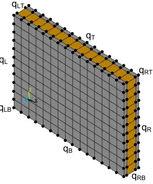
A periodic segment of a composite panel having arbitrary layering and material characteristics is hereby con-sidered (see Fig.2) with Lx, Lyits dimensions in the x and y directions respectively. The structural segment can be

modelled using a conventional FE package and the mass and stiffness matrices of the segmentM,Kcan be computed in a straightforward manner. A periodic structure wave scheme can be employed in order to numerically determine the propagating wavenumbers kwand the corresponding mode shapes xwfor each propagating wave mode type as

exhibited in Appendix A.

qR qL

qT

qLB qLT

qRB qRT

qB

Figure 2: Caption of a FE modelled composite layered panel

It is noted that matrices K =R∗_{KR and M=R}∗_{MR in Eq.(A.6) are Hermitian therefore their resulting}

eigen-values are real and the set of eigenvectors will be orthogonal. Eigenvalue sensitivity for standard eigenproblems is an established result in modern literature [17, 18] that will be employed in the present work. The eigenproblem in Eq.A.6 can be differentiated with respect to the angle of wave propagationθgiving

[K−λwM]

∂xw

∂θ + ∂K

∂θ −λw ∂M

∂θ !

xw−

∂λw

∂θ Mxw=0 (5)

After multiplying the above expression by x⊤_w and making use of the mass normalization of the eigenmodes the following expression can be derived for the angular sensitivity of the computed eigenalues

∂λw

∂θ =x ⊤

w

∂K ∂θ −λw

∂M ∂θ

!

xw (6)

In case of repeated eigenvalues being detected, the sensitivity expression should be modified according to the findings in [19, 20]. Taking into account thatMandKhave no angular dependence, the above expression can be developed to provide a more generic angular eigenvalue sensitivity expression

∂λw

∂θ =x ⊤

w

∂K

∂θxw−λwx ⊤

w

∂M ∂θ xw=x

⊤

w

∂R∗

∂θ KR+R ∗

K∂R ∂θ !

xw−λwx⊤w

∂R∗

∂θ MR+R ∗

M∂R ∂θ

!

For the wavenumber sensitivity ∂kw

∂θ the following expression stands ∂kw

∂θ = ∂kw

∂ωw

∂ωw

∂λw

∂λw

∂θ (8)

while the inverse of the group velocity ∂kw

∂ωw

can be computed [21, 22, 23] directly through the results of a single eigenvalue solution (that is avoiding FD for one more time) by differentiating the eigenproblem in Eq.A.6 with respect to kw, deriving

∂R∗ ∂kw

[K−ω2wM]R+R

∗

[K−ω2wM]

∂R ∂kw

−2ωw

∂ωw

∂kw

R∗MR !

xw+R∗[K−ω2wM]R

∂xw

∂kw

=0 (9)

and by multiplying the above expression by x⊤_w and taking advantage of the orthogonality properties the ∂kw

∂ωw

term can be directly obtained as

∂kw

∂ωw =                

2ωw

x⊤

w

∂R∗ ∂kw

[K−ω2_wM]R+R∗[K−ω2_wM]∂R

∂kw

! xw                 (10)

Eventually (taking into account that ∂ωw

∂λw

= 1

2ωw

), Eq.8 can therefore provide a direct expression of the angular wavenumber sensitivity for any propagating wave type w and direction of propagationθat angular frequencyωw

∂kw

∂θ =                

x⊤_w ∂R ∗

∂θ KR+R ∗

K∂R ∂θ

!

xw−λwx⊤w

∂R∗

∂θ MR+R ∗ M∂R ∂θ ! xw x⊤ w ∂R∗ ∂kw

[K−ω2_wM]R+R∗[K−ω2_wM]∂R

∂kw

! xw                 (11)

It is noted that R is a direct function of kwandθ, therefore the

∂R ∂kw

and∂R

∂θ terms are straightforward [24] to compute.

The global stiffness matrixKof the structural segment is formed by adding the local stiffness matrices of individual FEs as

K=

N

X

p=1

Kp with K

[(3p−2):3p,(3p−2):3p]

p =kp (12)

with N the total number of FEs and the superscript ofKpdenoting the exact positioning of kpwithin it. The remaining

entries inKpare null. The individual FE stiffness matrices can be computed as

kp =

Z 1 −1 Z 1 −1 Z 1 −1

B⊤C0B|J|dηdξdµ (13)

at the material principal axis which can contain up to 21 independent coefficients (for a triclinic material), input as

C0=                                        

c11 c12 c13 c14 c15 c16

c12 c22 c23 c24 c25 c26

c13 c23 c33 c34 c35 c36

c14 c24 c34 c44 c45 c46

c15 c25 c35 c45 c55 c56

c16 c26 c36 c46 c56 c66                                         (14)

If a revolution angleξ is considered between the material principal axis and the effective transformed coordinate system, then the transformed elastic stiffness matrix (rotated about z axis) can be calculated as [25]

C=T−1C0T−⊤ (15)

with T−1_{being the inverse of the coordinate transformation matrix given by}

T−1=

                                        

cos2_{(−ξ) sin}2

(−ξ) 0 0 0 2 cos(−ξ) sin(−ξ)

sin2(−ξ) cos2_{(−ξ) 0 0 0 −2 cos(−ξ) sin(−ξ)}

0 0 1 0 0 0

0 0 0 cos(−ξ) −sin(−ξ) 0

0 0 0 sin(−ξ) cos(−ξ) 0

−cos(−ξ) sin(−ξ) cos(−ξ) sin(−ξ) 0 0 0 cos2_{(−ξ)−sin}2 (−ξ)

                                         (16)

Eventually, substituting Eq.11 into Eq.4 and subsequently into Eq.1 provides a generic expression of the energy skew angle for each wave type w as

ψw=

π

2 −θ−arctan                                          tanθ                

x⊤_w ∂R ∗

∂θ KR+R ∗

K∂R ∂θ

!

xw−λwx⊤w

∂R∗

∂θ MR+R ∗ M∂R ∂θ ! xw x⊤ w ∂R∗ ∂kw

[K−ω2wM]R+R

∗

[K−ω2wM]

∂R ∂kw

! xw                

+kw

kwtanθ−

               

x⊤_w ∂R ∗

∂θ KR+R ∗

K∂R ∂θ

!

xw−λwx⊤w

∂R∗

∂θ MR+R ∗ M∂R ∂θ ! xw x⊤ w ∂R∗ ∂kw

[K−ω2_wM]R+R∗[K−ω2_wM]∂R

∂kw

! xw                                                          (17)

which quantifies the wave energy skewing as a direct function of the mechanical characteristics of the layered struc-ture. It is reminded that the above expression is valid for 0≤θ < π(see Eq.1 for the remaining quadrants).

4. Numerical case studies

elastic stiffness matrix

C0=109                                        

94 7.4 8.2 0 0 0 7.4 13 9.1 0 0 0 8.2 9.1 34 0 0 0

0 0 0 3.6 0 0

0 0 0 0 7.2 0

0 0 0 0 0 4.2

                                       

N/m2

while the density of the structure isρ=1600kg/m3 and its thickness is h=1mm. The dimensions of the modelled periodic segment are Lx=Ly=10mm with a mesh comprising 10 elements in each direction. The results on the slowness

curves as well as on the energy skew angles are presented in Figs.3 and 4 at frequencies of 0.1MHz and 0.5MHz respectively. The results are compared to a FD scheme [15] in which the group velocity at a given wave propagation direction is determined as

∂ωw

∂kw

= lim

ωw2→ωw1

ωw2−ωw1

kw2−kw1

(18)

while a similar finite central difference scheme is employed for calculating the angular dependence of the frequency at which a certain wavenumber occurs

∂ωw

∂θ =δθlim→0

ωw(k)|θ1+δθ/2−ωw(k)|θ1−δθ/2

δθ (19)

Acceptable values forωw2andδθshould be derived through a relative error convergence study withωw2−ωw1andδθ

gradually diminishing until the relative difference in the acquired results is inferior to a defined tolerance.

It is stressed that the scheme proposed in this work is able to compute the wavenumber angular sensitivity (and subsequently the energy skew angle) by determining and post-processing a single solution of the system. This over-comes the two primary drawbacks of FD approaches; the first being that FD schemes require multiple solutions of the system for computing each gradient (more accurate FD schemes such as centered second and higher order ones ask for three or five solutions for computing just a single gradient). The second drawback that is overcome by the presented approach is that the variable perturbation for a FD scheme should be determined through a solution convergence study which also requires multiple solutions of the system under investigation. When it comes to large industrial models comprising an important number of elements, FD schemes are therefore expected to be computationally cumber-some. In that case the approach presented herein is deemed more appropriate, providing simultaneous efficiency and accuracy advantages.

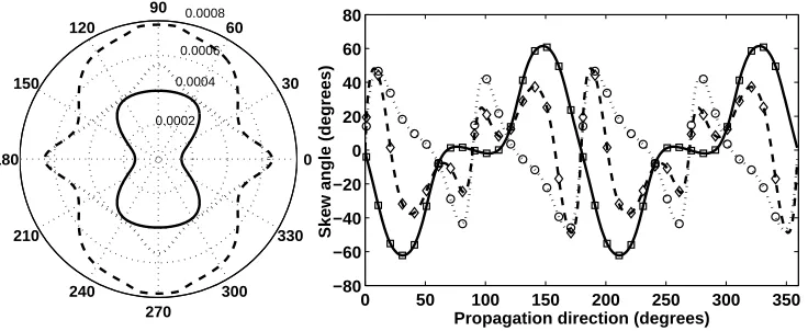
The results in Figs.3 and 4 unveil the intense angular, frequency and wave-type dependence of the slowness curves for the three propagating elastic waves. The SH0wave velocity appears to converge towards the A0phase velocities in the ’stiffer’ direction of the structure. The intense variation of the energy skewing effect is also demonstrated in the same figures with the maximum skew angle being greater than 55o_{for all wave types. Due to the symmetry of the}

slowness curves all skew angles areψ=0 atθ=0o_/180o_{as well as atθ=90}o_/270o_{. It is observed that the skew angle}

0.0005 0.001 0.0015

0.002

30

210

60

240 90

270 120

300 150

330

180 0

0 50 100 150 200 250 300 350

−80 −60 −40 −20 0 20 40 60 80

Propagation direction (degrees)

Skew angle (degrees)

Figure 3: Left: Wave slowness curves for the P0(–), SH0(· · ·) and A0(- -) waves propagating in the orthotropic graphite-epoxy monolithic structure

at 0.1MHz. Right: Corresponding energy skew angles computed through the presented approach for the P0(–), SH0(· · ·) and A0(- -) waves. Also

presented the skew angles computed through a FD scheme as exhibited in [15] for the P0(), SH0(◦) and A0(⋄) waves.

0.0002 0.0004

0.0006 0.0008

30

210

60

240 90

270 120

300 150

330

180 0

0 50 100 150 200 250 300 350 −80

−60 −40 −20 0 20 40 60 80

Propagation direction (degrees)

Skew angle (degrees)

Figure 4: Left: Wave slowness curves for the P0(–), SH0(· · ·) and A0(- -) waves propagating in the orthotropic graphite-epoxy monolithic structure

at 0.5MHz. Right: Corresponding energy skew angles computed through the presented approach for the P0(–), SH0(· · ·) and A0(- -) waves. Also

−2500 −2000 −1500 −1000 −500 0 500 1000 1500 2000 2500 −2500

−2000 −1500 −1000 −500 0 500 1000 1500 2000 2500

cg,y

c g,x

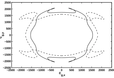
Figure 5: Group velocity curves for the A0(–) and the SH0(- -) waves propagating in the orthotropic graphite-epoxy monolithic structure,

visual-izing the appearance of caustics at 0.1MHz.

more intense aroundθ=0o/180ofor higher frequencies. Moreover, an excellent correlation is observed between the exhibited computational scheme and the FD scheme.

It should be noted that through the knowledge of the amplitude and actual direction of cgit is also straightforward

to determine and visualize the appearance of caustics [26] in the group velocity diagrams. An example of this wave behaviour is exhibited in Fig.5 for the A0and SH0propagating guided waves.

5. Conclusions

The principal outcomes of the work are summarized as follows:

(i) A generic expression quantifying the wave energy skew angle as a function of the mechanical characteristics of a non-isotropic structure has been derived in this study. The approach does not involve any FD procedure and is therefore efficient and not prone to the associated numerical errors.

(ii) A FE-based approach for efficiently computing the angular sensitivity of the wave slowness for each wave type, direction and frequency was employed. The considered structure can be of arbitrary layering and material character-istics as an FE modelling approach is adopted. By employing periodic structure theory the associated computational effort is radically reduced.

(iii) An intense frequency dependence of the energy skew angle was observed for the A0waves travelling in an orthotropic graphite-epoxy monolithic structure. Angular and wave-type dependence was observed for the entirety of propagating waves with the skew angle being as pronounced as 65o _{in some cases. It was also shown that the}

presented approach can successfully determine and visualize the appearance of caustics in the group velocity curves.

References

[1] F. Yan, R. L. Royer, J. L. Rose, Ultrasonic guided wave imaging techniques in structural health monitoring, Journal of intelligent material

[2] M. Kersemans, W. Van Paepegem, K. Van Den Abeele, L. Pyl, F. Zastavnik, H. Sol, J. Degrieck, Pitfalls in the experimental recording of

ultrasonic (backscatter) polar scans for material characterization, Ultrasonics 54 (2014) 1509–21.

[3] E. Lean, W. Chen, Large-angle acoustic-beam steering in acoustically anisotropic crystal, Applied Physics Letters 35 (1979) 101–3.

[4] D. H. Turnbull, F. S. Foster, Beam steering with pulsed two-dimensional transducer arrays, Ultrasonics, Ferroelectrics, and Frequency

Control, IEEE Transactions on 38 (1991) 320–33.

[5] S. W. Smith, H. G. Pavy Jr, O. T. Von Ramm, High-speed ultrasound volumetric imaging system. i. transducer design and beam steering,

Ultrasonics, Ferroelectrics, and Frequency Control, IEEE Transactions on 38 (1991) 100–8.

[6] A. C. Clay, S.-C. Wooh, L. Azar, J.-Y. Wang, Experimental study of phased array beam steering characteristics, Journal of Nondestructive

Evaluation 18 (1999) 59–71.

[7] S.-C. Wooh, Y. Shi, Optimum beam steering of linear phased arrays, Wave motion 29 (1999) 245–65.

[8] K. Salas, C. Cesnik, Guided wave structural health monitoring using clover transducers in composite materials, Smart Materials and Structures

19 (2009) 1–25.

[9] S. Wu, M. Wu, C. Huang, J. Yang, Fpga-based implementation of steerable parametric loudspeaker using fractional delay filter, Applied

Acoustics 73 (2012) 1271–81.

[10] M. Ruzzene, F. Scarpa, F. Soranna, Wave beaming effects in two-dimensional cellular structures, Smart materials and structures 12 (2003)

363–72.

[11] M. I. Hussein, M. J. Leamy, M. Ruzzene, Wave beaming in nanostructured materials with engineered defects, in: ASME 2008 International

Mechanical Engineering Congress and Exposition, American Society of Mechanical Engineers, pp. 1011–8.

[12] F. Casadei, J. Rimoli, Anisotropy-induced broadband stress wave steering in periodic lattices, International Journal of Solids and Structures

50 (2013) 1402–14.

[13] B. P. Newberry, R. B. Thompson, A paraxial theory for the propagation of ultrasonic beams in anisotropic solids, The Journal of The

Acoustical Society of America 85 (1989) 2290–300.

[14] J. L. Rose, Ultrasonic waves in solid media, Cambridge university press, 2004.

[15] L. Wang, F. Yuan, Group velocity and characteristic wave curves of lamb waves in composites: Modeling and experiments, Composites

Science and Technology 67 (2007) 1370–84.

[16] J. M. Carcione, Wave fields in real media: Wave propagation in anisotropic, anelastic, porous and electromagnetic media, volume 38, Elsevier,

2007.

[17] R. B. Nelson, Simplified calculation of eigenvector derivatives, AIAA journal 14 (1976) 1201–5.

[18] S. Adhikari, M. I. Friswell, Eigenderivative analysis of asymmetric non-conservative systems, International Journal for Numerical Methods

in Engineering 51 (2001) 709–33.

[19] J.-N. Juang, P. Ghaemmaghami, K. B. Lim, Eigenvalue and eigenvector derivatives of a nondefective matrix, Journal of Guidance, Control,

and Dynamics 12 (1989) 480–6.

[20] M. Friswell, The derivatives of repeated eigenvalues and their associated eigenvectors, Journal of vibration and acoustics 118 (1996) 390–7.

[21] S. Finnveden, Evaluation of modal density and group velocity by a finite element method, Journal of Sound and Vibration 273 (2004) 51–75.

[22] V. Cotoni, R. S. Langley, P. J. Shorter, A statistical energy analysis subsystem formulation using finite element and periodic structure theory,

Journal of Sound and Vibration 318 (2008) 1077–108.

[23] M. Ichchou, S. Akrout, J.-M. Mencik, Guided waves group and energy velocities via finite elements, Journal of Sound and Vibration 305

(2007) 931–44.

[24] D. Chronopoulos, Design optimization of composite structures operating in acoustic environments, Journal of Sound and Vibration 355

(2015) 322–44.

[25] R. M. Jones, Mechanics of composite materials, volume 193, Scripta Book Company Washington, DC, 1975.

[26] A. Spadoni, M. Ruzzene, S. Gonella, F. Scarpa, Phononic properties of hexagonal chiral lattices, Wave motion 46 (2009) 435–50.

Vibration 167 (1993) 377–81.

Appendix A. Determining the angular sensitivity of the propagating wave characteristics through a finite

ele-ment scheme

Appendix A.1. Computation of propagating wave properties through a finite element approach

The wave propagation analysis scheme presented below has been first exhibited in [27]. The DoF set q (as well as theM,Kmatrices) is reordered according to a predefined sequence such as:

q={qI qB qT qL qR qLB qRB qLT qRT}⊤ (A.1)

corresponding to the internal, the interface edge and the interface corner DoF (see Fig.2). The free harmonic vibration equation of motion for the modelled segment is written as:

[K−ω2_{M]q=0 (A.2)}

The analysis then follows as in [22] with the following relations being assumed for the displacement DoF under the passage of a time-harmonic wave:

qR=e−iεx_{qL, qT=e}−iεy_qB

qRB=e−iεxqLB, qLT=e−iεyqLB, qRT=e−iεx−iεyqLB

(A.3)

withεxandεythe propagation constants in the x and y directions related to the phase difference between the sets of

DoF. The wavenumbers kx, kyare directly related to the propagation constants through the relation:

εx=kxLx, εy=kyLy (A.4)

Considering Eq.A.3 in tensorial form gives:

q=                                                                

I 0 0 0

0 I 0 0

0 Ie−iεy _{0 0}

0 0 I 0

0 0 Ie−iεx ₀

0 0 0 I

0 0 0 Ie−iεx

0 0 0 Ie−iεy

0 0 0 Ie−iεx−iεy                                                                

x=Rx (A.5)

[R∗_KR−ω2_R∗_{MR]x=0 (A.6)}

with∗_{denoting the Hermitian transpose. The most practical procedure for extracting the wave propagation}

character-istics of the segment from Eq.A.6 is injecting a set of assumed propagation constantsεx,εy. The set of these constants

can be chosen in relation to the direction of propagation towards which the wavenumbers are to be sought and ac-cording to the desired resolution of the wavenumber curves. Eq.A.6 is then transformed into a standard eigenvalue problem and can be solved for the eigenvector xwwhich describe the deformation of the segment under the passage

of each wave type w at an angular frequency equal to the square root of the corresponding eigenvalueλw = ω2w.

A complete description of each passing wave including its x and y directional wavenumbers and its wave shape for a certain frequency is therefore acquired. It is noted that the periodicity condition is defined modulo 2π, therefore solving Eq.A.6 with a set ofεx,εyvarying from 0 to 2πwill suffice for capturing the entirety of the structural waves.

Nomenclature

B Shape function derivative matrix of a single FE

C0 Elastic stiffness matrix at the material principal axis

J Jacobian matrix of a single FE

K Intermediate stiffness matrix employed for the assembly ofK M,K Mass and stiffness matrices of the periodic element

R Displacement phase transformation matrix

T Coordinate transformation matrix

k Stiffness matrix of a single FE

q Physical displacement vector for the elastic waveguide

Lx, Ly Dimensions of the modelled periodic segment

L, R, B, T , I Left, right, bottom, top sides and interior indices

N Number of elements

cg Group velocity

k Wavenumber

lx,ly,lz Dimensions of a single FE

s Wave slowness

w Wave type index

x Wave mode shape vector for the elastic waveguide

ε Propagation constant

θ Wave propagation angle

η,ξ,µ Local FE coordinates

λ Eigenvalue of the wave propagation eigenproblem

ψ Energy skew angle

ξ Coordinate transformation angle