Bridge asset management using petri-nets
P Yianni1; L C Neves2; D Rama2; J Andrews2; R Dean3
1: Amey Strategic Consulting & Technology, Furnival St., London, EC4A 1AB, United Kingdom.
2: Resilience Engineering Research Group, University of Nottingham, Faculty of Engineering, University Park, Nottingham, NG7 2RD, United Kingdom.
3: Network Rail, The Quadrant:MK, Elder Gate, Milton Keynes, Buckinghamshire, MK9 1EN, United Kingdom.
Abstract
Management of a diverse portfolio of assets is a demanding and complex task. Although extensive research has been carried out in bridge asset management models, the model developed in this study contains flexibility which is able to model a vast array of different types of elements, under different environmental stressors and with different operational strategies. The Petri-Net model developed contains a number of different modules
interconnecting to form a robust bridge asset management modelling framework. The result is an adaptable and flexible decision making tool approach to help bridge portfolio managers.
The UK railway network is integral to commerce as it carries both commuters as well as freight. Their reliance on the network causes great operational pressure and that pressure is only intensifying. Planned upgrades, for example, ERTMS (1), should enable more throughput for the system, but at the potential cost of more rapid deterioration of the railway assets. Therefore, a more thorough understanding of the assets is required to be able to manage them through this period of increased operational intensity. This study focuses on bridge assets, in particular, bridges which are used on the railway network.
One of the most important aspects of managing assets is understanding their failure modes and deterioration characteristics. Modern bridges built in the UK are governed by design protocols (2), however, there is very little governance on the usage of assets once they have been constructed. Understanding the deterioration characteristics is made more challenging when an existing portfolio of assets must be effectively managed which have been built from different materials, utilised under different operational strategies and maintained under different intervention policies. Managing such a diverse portfolio is a demanding and complex challenge.
1 STOCHASTIC MODELS
Bridge asset management has been an evolving field with a number of key studies involving stochastic modelling techniques. These have often involved the use of Markov models with the key notion being that: 1) structural deterioration is naturally stochastic (3) and 2) that the “micro-response” of the structure introduces much uncertainty into the deterioration characteristics (4) and is, therefore, the most suitable modelling approach.
Another widely recognised bridge asset management study was carried out in Virginia, USA with a much larger portfolio of 13,000 bridges (7). A Markov approach was employed using 7 condition states ranging from 7, representing a new condition, to 1 representing a potentially hazardous condition. Considering the population size in the study, the authors state that a normal Markov chain approach would create too many states to compute. Therefore, a process of grouping was carried out so that the 13,000 bridges were categorised into 216 individual groups. This demonstrated an effective approach at overcoming the Markov state space explosion problem. However, the authors recognise that categorisation of the bridge assets can be subjective and that assets may have different operational characteristics over the course of their lifetimes.
Many of the bridge asset management models favour the Markov modelling approach. However, this technique has several drawbacks some of which are specific to the modelling approach and others which are specific to modelling bridge assets. These include: 1) calibration using historical bridge data which requires expert judgement for cases where assets are on the border between condition states (3), 2) the parameters of the Markov models can be difficult to calculate accurately and so require additional adjustment using expert judgement (3) 3) inspection data is used primarily in the studies to determine the deterioration and condition of the bridge assets, however, many studies disregard the inspections which indicate an improvement in condition as it is difficult to be certain if an intervention has occurred (8,9) and finally 4) the Markovian limitation of state space explosions (10) which creates difficulties with large bridge portfolios; although some studies have used techniques to overcome this limitation, it introduced other drawbacks (7). Overall, it can be seen that management of bridge assets is internationally significant and that an effective modelling approach could provide valuable insights.
2 PETRI-NETS
Petri-Nets (PNs) are directed, bipartite graphs which use two types of nodes. The first type of node, which gives the PN its structure, is called a “place” and is used to indicate possible system states. For example, a set of places could represent the possible conditions of a bridge asset. The actual indication is made by the location of tokens within the system, for example a token occupying a place labelled “poor condition” would indicate that the particular bridge asset was in a poor condition. To move tokens from place to place, transitions are used. For example, if a bridge asset deteriorated from a poor condition to a hazardous condition, in the model this would be represented by a token being moved by a transition from a place labelled “poor condition” to a place labelled “hazardous condition”. The links between the nodes are known as arcs and no two places or transitions can be linked directly. The components can be seen in Figure 1 and more information can be found in (11).
Figure 1: Components of a Petri-Net. From left to right: unmarked place; marked place; arc; transition.
2.1 Coloured Petri-Nets
Coloured Petri-Nets (CPNs) are an extension to the PN modelling technique (12). It adds in the ability to perform more sophisticated operations. This is largely because tokens now have their own identity and contain tuple information within them. For example, to model each element of the bridge asset in one modelling space without interference is now possible with the use of CPNs, which overcomes the Markov state space explosion issue (13) discussed in Section 1. As each token now has its own identity, this also allows transitions to act differently upon them depending on their characteristics. In a bridge management context, if two different bridge elements, for example a wing wall and a soffit, represented by two tokens, occupied a place marked “good condition”, the transition could move the tokens to the place labelled “poor condition” at different times depending on the type of bridge element. This extension to normal PNs allows for more flexibility in the modelling technique which allows more accurate modelling of the bridge elements.
3 DETERIORATION, MAINTENANCE AND EXAMINATION POLICIES
dependent on the material type, a different SevEx matrix is provided for each one. For concrete, which is the exemplar element in this study, there are a total of 31 SevEx conditions ranging from A1, an “as new” condition to G6 which represents elements in a state of permanent structural deformation. The most common cause of defects for concrete elements is cracking and spalling which is evident from the historic data as well as other sources of literature (14).
The NR policies on inspection state that bridges should be inspected according to their condition. Bridges that are in poorer condition will require more maintenance whereas those which are in better condition will require less (15). The policies outline a conversion from the inspection data to a risk score which can then be used to calculate an appropriate inspection interval. To be able to perform dynamic selection of inspection intervals in the proposed model, a back-conversion was carried out so that the inspection interval is directly related to the condition, expressed as the SevEx score. For concrete elements, the policy broadly outlines that bridges in a good condition should be inspected every 12 years, bridges that are in a medium condition should be inspected every 6 years and bridges which are in poor condition should be inspected every 3 years.
The NR policies regarding remedial works depending on the condition of the element. There are three types of remedial works: 1) Replacement of elements that fall below the “Basic Safety Limit”, which is a minimum requirement for all elements, covers SevEx conditions: D6, E5-E6, F4-F6, G2-G6 2) Major Repair for elements which are experiencing moderately severe defects which covers SevEx conditions B5-B6, C4-C6, D3-D5, E2-E4, F2-F3 and 3) Minor Repair which is carried out on elements experiencing mild severity defects, which covers SevEx conditions B2-B4, C2-C3, D2. All SevEx condition states have a corresponding type of remedial work apart from Sevex condition state A1.
4 SOURCE OF DATA
A number of databases were used for this study including: 1) the asset register database known as the Civil Asset Register and Reporting System (CARRS) 2) the database which holds inspection and bridge element SevEx condition information, known as the Structure Condition Marking Index (SCMI) database 3) the database containing information on Minor Repairs, known as MONITOR, and 4) the database for larger remedial works known as the Cost Analysis Framework (CAF) database. The total number of bridges in this combined database was 25,949 which contained information for 273,427 Major Element and 563,150 Minor Elements. The SevEx condition data is for each Minor Element of which there are 1,397,748 total inspections on Minor Elements. This study uses concrete bridges as the exemplar bridge group of which there are 4,434 in the combined database. The number of repeat inspections of concrete main girders, the exemplar Minor Element type in this study, is 407,708. Repeat inspections are important as they enable the analysis of defect evolution and behaviour.
5 PETRI-NET BRIDGE MANAGEMENT MODEL
The proposed model uses a bottom-up approach rather than a top-down approach which means that it works on the bridge and element level rather than the portfolio level. The PN model framework has been created so that a bridge of any size (i.e. any number of any number of tokens, representing bridge elements) can be modelled. The model is organised into modules with the three main modules being 1) the deterioration module, which holds all the Sub-Minor Element conditions and controls their rate of deterioration as well as future defect development, 2) the inspection module which updates the revealed condition of the elements in accordance with the industry standard policies and 3) the repair module which is triggered once an inspection has occurred and the appropriate remedial work has been scheduled; this provides a condition uplift to the appropriate elements in the deterioration module once the simulated remedial work has been carried out.
Calibration of the deterioration module used historic data and considered all 31 possible SevEx states. The interactions between the states was considered and it was deemed that only movements to the poorer condition neighbouring condition states were valid i.e. an element in a B3 condition could only move to a B4, C3 or C4 condition. This data was used to calculate Mean Time to Failure (MTTF) between each of the condition states. For example, the MTTF for an element to deteriorate from condition state B3 to B4 would be calculated with the
equation shown in Equation 1. Where t is the inspection interval, nB3 is the number of elements that initially started
in condition state B3 and mB3->B4 is the number of elements that moved from condition state B3 to B4.
𝑀𝑇𝑇𝐹𝐵3→𝐵4=
𝑡 ∙ 𝑛𝐵3 𝑚𝐵3→𝐵4
The MTTF can simply be used to find the failure rate (λ), which is then embedded into the corresponding PN
transition in the model i.e. λB3->B4 would be embedded into the transition that connected the places which
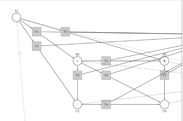
[image:4.482.95.393.104.301.2]represented condition states B3 and B4 in the deterioration module of the PN model. The deterioration module can be seen in Figure 2. It shows the links between the places, representing the SevEx condition states, and the transitions. Two example bridge elements, shown as tokens, are shown in the figure; one element is represented by the black token, another element represented by the red token. They represent different bridge elements which are of different types as well as at different stages of deterioration. Only places A1 to C3 are shown for illustrative purposes, however the full model includes all 31 SevEx states.
Figure 2: Deterioration Module showing the link between the places and transitions.
[image:4.482.142.344.463.638.2]The inspection module controls when and how frequently inspections occur. This is in accordance with the industry standard guidelines which indicate that assets in a good condition require fewer inspections than assets in a poor condition. The same inspection policies have been embedded into this module so that it simulates inspections in accordance with the industry standard guidelines. This is realised in the model using the transition labelled T11 in Figure 3. This transition contains advanced functionality which is able to determine the correct inspection interval in relation to the known element condition, which is only possible with the use of CPNs. This is represented in the PN model with the dashed input arcs which indicate that the transition only takes in information from these places rather than tokens. T11 is directly connected to the place labelled “Between Inspections” and when the next inspection is due, the transition then absorbs the token and inserts another into the place marked “During Inspection” to indicate that a simulated inspection is taking place. T12 is a simple transition which simply absorbs the token from the place labelled “During Inspection” when the simulated inspection has been completed and inserts it into the place labelled “Between Inspection”. This duration has been calibrated with expert judgement.
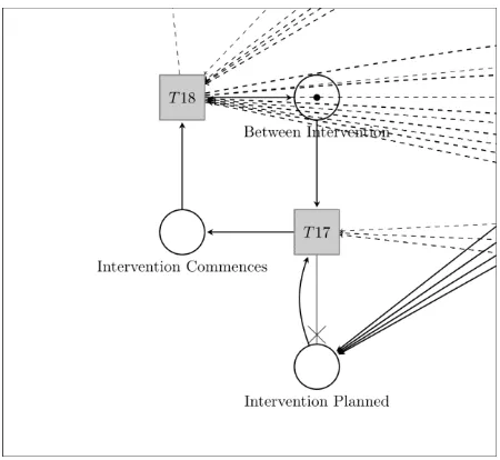
Once an inspection has occurred, if maintenance is required then it is scheduled accordingly. The three types of remedial works which the industry use are mimicked in the PN model to improve the accuracy of the model. The intervention module can be seen in Figure 4 and uses a lot of CPN features to replicate the complexity of the process. The transition labelled T17 models the delay from scheduling an intervention after an inspection and it occurring. This is calibrated using historic maintenance data so that each type of maintenance action has the correct delay time attributed to it. The delay arises due to planning the remedial works, ordering the materials and scheduling the timetable slot to perform the works. More minor remedial works require less planning, fewer materials and less time which means that they can be performed faster. The complexity of the module is mostly attributed to transition T18 which is designed to mimic the process when the maintenance teams get on site to perform the remedial works. There are two possibilities 1) the element is in the condition that they were expecting and so they can carry out the planned works, or 2) the element has deteriorated further during the delay time and the defect has worsened in severity which means that the time and resources allocated are no longer sufficient. In this instance, the correct maintenance action would be scheduled and the teams would have to return. This feature was included in the model to make the model more accurate to the real-world process.
Figure 4: Intervention module which carried out the three different types of remedial work used by the industry.
6 SIMULATION RESULTS
The PN model proposed is able to model a whole bridge asset by inserting the appropriate tokens, representing the bridge elements, into the model. Simulations can then be run on the model and the aggregated outputs be used to understand the system behaviour. For illustrative purposes, a single concrete main girder has been simulated. As more elements are added to the model, the deterioration profiles overlap making the overall output more difficult to understand. The concrete main girder was simulated from an A1, “as new”, condition over a 100-year period.
Figure 5: Simulated Condition over time of a typical concrete main girder element.
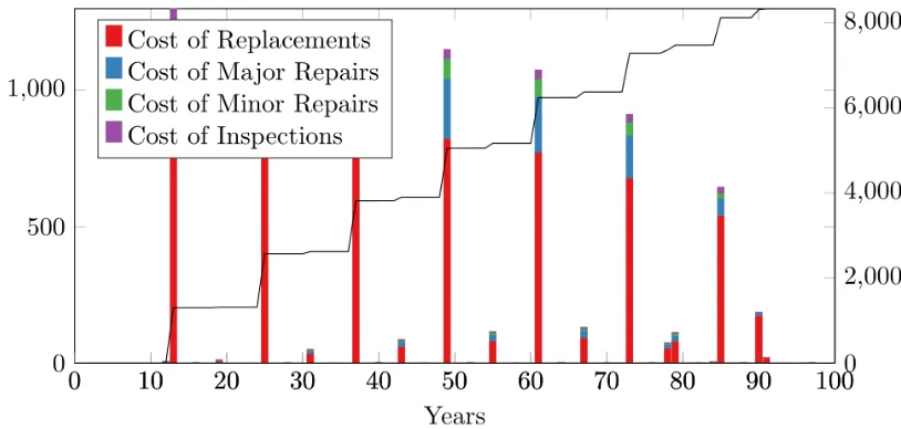
A key attribute of the model as a decision making tool for bridge portfolio managers is the ability to predict when maintenance will be required, the type of maintenance and the associated cost of the works. The maintenance actions of the PN model are calibrated in accordance with the industry standard policies which affords the model an increased level of accuracy in predictions. An example of this output can be seen in Figure 6 and is the simulation results for the same concrete girder element as seen in Figure 5. It can be seen that the inspections are only carried out in the 12 year cycles as per the industry standard policies. However, the outcome of the inspections is often some type of remedial work. The standard maintenance strategy is to maintain the elements whenever they require maintenance. It can be seen from the figure that there are simulation iterations where replacement of the element is required, and the disproportionate cost of replacement works drives up the cumulative lifetime cost, known as the Whole Life Cycle Cost (WLCC). The vast majority of remedial works in this simulation were Minor Repairs with far fewer Major Repairs. One additional aspect of interest is the small costs that seem to be out of phase with the main peaks. These occur in simulation iterations where the maintenance team had to return to perform the remedial works as described in Section 5.
Figure 6: Model Output showing when maintenance is predicted to be required, the type of maintenance and the cost associated with the maintenance.
7 ASSET DETERIORATION FACTORS
[image:6.482.43.450.347.541.2]The elements were matched with the corresponding corrosion ranks to determine which group they would be in for the analysis. To determine if the deterioration rate of the elements correlated to the galvanic corrosion in their region, the MTTF times and the SevEx matrix were used to calculate the typical time it would take the groups of elements to reach a threshold requiring maintenance. The analysis provided enough evidence to determine that there was some correlation between the element deterioration rates and the galvanic corrosion in the region.
Rather than compare the deterioration rates directly, it was determined that for bridge portfolio managers, the crucial result would be the financial impact of this difference. Therefore, the main girder elements, grouped by their galvanic corrosion rank, were used to calibrate different profiles into the Deterioration Module, seen in Figure 2. The profiles were 1) the typical deterioration profile experienced across the whole of the UK, 2) the deterioration profile for bridge elements in areas of mild corrosion, 3) the deterioration profile for bridge elements in areas of moderate corrosion and finally 4) the deterioration profile for bridge elements in areas of aggressive corrosion.
The PN model was then simulated with a typical concrete main girder element being exposed to each of these profiles. The maintenance strategy used in this simulation was a “Managed” strategy in which the element is only repaired when it requires Major Repair or Replacement. This was used for the comparison in this example as it is more operationally realistic and therefore the results are more meaningful.
Table 1: WLCC output results from the PN model with an example element exposed to different deterioration profiles.
ID Corrosion
Level (nearest WLCC
100mu)
Relative Cost to Control
1 (Control) All 7,900 1.0
2 Mild 1,800 0.235
3 Moderate 4,000 0.512
4 Aggressive 27,500 3.501
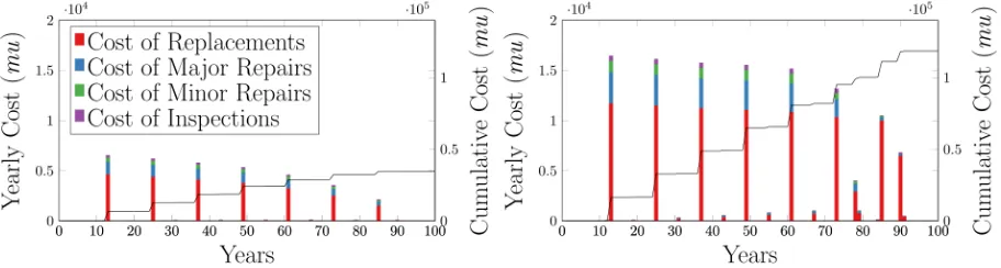
[image:7.482.18.474.404.526.2]The WLCC output can be seen in Table 1. The control scenario, which is calibrated with all the historic element data, regardless of its corrosion level, results in a typical WLCC of 7,900 monetary units. Elements which are in areas exposed to mild corrosion only seem to cost a quarter of the WLCC of the control scenario, which is significantly less. Elements which are exposed to moderate levels of corrosion have a WLCC of just over half the control scenario. However, the most significant result is the WLCC of elements in areas exposed to aggressive corrosion as they have a WLCC of more than three and a half times the control scenario. The PN model outputs, seen in Figure 7, show the difference in the type of maintenance elements in these areas typically require over the 100-year period as well as the overall WLCC.
Figure 7: Comparison of the WLCC between a typical concrete main girder element in an area of moderate corrosion (left) to one in an area of aggressive corrosion (right).
8 CONCLUSION
developed model a great deal of accuracy to the real-world system. In addition to this, analysis into the factors which affect bridge deterioration allows the model to hone in on bridge elements exposed to particular environmental stressors. In conclusion, a novel new approach to bridge asset management has been developed which provides new insights critical for bridge portfolio managers.
ACKNOWLEDGEMENTS
John Andrews is the Royal Academy of Engineering and Network Rail Professor of Infrastructure Asset Management. He is also Director of The Lloyds Register Foundation (LRF) Centre for Risk and Reliability Engineering at the University of Nottingham. Robert Dean is the Professional Engineer within Technical Services at Network Rail. Matthew Hamer is the Whole Life Cost Specialist at Network Rail. Luis Canhoto Neves is an Assistant Professor at the Nottingham Transport Engineering Centre (NTEC) at the University of Nottingham. Dovile Rama is the Network Rail Research Fellow in Asset management. Panayioti Yianni is a Strategic Consultant within Amey Strategic Consulting. The research was supported by Network Rail and the Engineering and Physical Sciences Research Council (EPSRC) grant reference EP/L50502X/1. They gratefully acknowledge the support of these organizations.
REFERENCE LIST
1. Technical Strategy Leadership Group (TSLG). Rail Technical Strategy. Rail Research UK Association; 2012.
2. Eurocode. Eurocode 2: Design of concrete structures – Part 2: Bridges. 1996.
3. Frangopol DM, Kallen M-J, Noortwijk JM van. Probabilistic models for life-cycle performance of deteriorating
structures: review and future directions. Prog Struct Eng Mater. 2004;6(4):197–212.
4. Morcous G, Lounis Z, Cho Y. An integrated system for bridge management using probabilistic and
mechanistic deterioration models: Application to bridge decks. KSCE J Civ Eng. 2010;14(4):527–37.
5. Jiang Y, Sinha KC. Bridge service life prediction model using the Markov chain. Transp Res Rec.
1989;(1223):24–30.
6. Sobanjo JO, Thompson PD. Enhancement of the FDOT’s Project Level and Network Level Bridge Management
Analysis Tools. 2011 [cited 2015 Nov 23]; Available from: http://trid.trb.org/view.aspx?id=1101251
7. Scherer W, Glagola D. Markovian Models for Bridge Maintenance Management. J Transp Eng.
1994;120(1):37–51.
8. Robelin C-A, Madanat SM. History-dependent bridge deck maintenance and replacement optimization with
Markov decision processes. J Infrastruct Syst. 2007;13(3):195–201.
9. Morcous G, Rivard H, Hanna A. Modeling bridge deterioration using case-based reasoning. J Infrastruct Syst.
2002;8(3):86–95.
10. British Standards Institution. Analysis techniques for dependability — Petri net techniques. 2012.
11. Reisig W. Understanding Petri Nets: Modeling Techniques, Analysis Methods, Case Studies. 2013.
12. Jensen K. A brief introduction to coloured Petri Nets. In: Brinksma E, editor. Tools and Algorithms for the Construction and Analysis of Systems [Internet]. Springer Berlin Heidelberg; 1997 [cited 2014 May 12]. p. 203–8. (Lecture Notes in Computer Science). Available from:
http://link.springer.com/chapter/10.1007/BFb0035389
13. British Standards Institution. Systems and software engineering. High-level Petri nets. Concepts, definitions and graphical notation. British Standards Institution; 2004.
14. Nielsen D, Raman D, Chattopadhyay G. Life cycle management for railway bridge assets. Proc Inst Mech Eng Part F J Rail Rapid Transit. 2013;227(5):570–81.
15. Network Rail. Handbook for the examination of Structures Part 1C: Risk categories and examination intervals. NR/L3/CIV/006/1C. 2010;