Adaptive stabilization of uncontrolled rectifier based AC DC power systems feeding constant power loads

(1)

Adaptive Stabilization of Uncontrolled Rectifier

Based AC–DC Power Systems Feeding Constant

Power Loads

1

2

3

Kongpan Areerak, Theppanom Sopapirm, Serhiy Bozhko, Member, IEEE, Christopher Ian Hill, Member, IEEE,

Apichai Suyapan, and Kongpol Areerak

4 5

Abstract—It is known that, when tightly regulated, actively con-6

trolled power converters behave as constant power loads (CPLs). 7

These loads can significantly degrade the stability of their feeder 8

system. The loop-cancelation technique has been established as 9

an appropriate methodology to mitigate this issue within dc–dc 10

converters that feed CPLs. However, this has not yet been applied 11

to uncontrolled rectifier based ac–dc converters. This paper there-12

fore details a new methodology that allows the loop-cancelation 13

technique to be applied to uncontrolled rectifier based ac–dc 14

converters in order to mitigate instability when supplying CPLs. 15

This technique could be used in both new applications and easily 16

retrofitted into existing applications. Furthermore, the key con-17

tribution of this paper is a novel adaptive stabilization technique, 18

which eliminates the destabilizing effect of CPLs for the studied 19

ac–dc power system. An equation, derived from the average 20

system model, is introduced and utilized to calculate the adaptable 21

gain required by the loop-cancelation technique. As a result, 22

the uncontrolled rectifier based ac–dc feeder system is always 23

stable for any level of CPL. The effectiveness of the proposed adap-24

tive mitigation has been verified by small-signal and large-signal 25

stability analysis, simulation, and experimental results. 26

Index Terms—AC–DC converters, constant power load (CPL), 27

loop-cancelation technique, negative impedance instability. 28

I. INTRODUCTION 29

A

CTIVELY controlled power converters are widely used in

30

many applications. Unfortunately, when tightly regulated,

31

actively controlled power converters behave as constant power

32

loads (CPLs) [1], [2]. These CPLs can significantly degrade

33

the stability of their feeder system [3]–[5]. It can be seen from

34

previous publications [6]–[10], that unstable system operation

35

can be predicted from dynamic mathematical models via

con-36

trol theory. In order to derive models in such a way as to be

37

Manuscript received July 25, 2017; revised October 19, 2017; accepted November 25, 2017. This work was supported in part by Suranaree University of Technology and in part by the office of the Higher Education Commission under NRU Project of Thailand. Recommended for publication by Associate Editor F. J. Azcondo. (Corresponding author: Kongpan Areerak.)

K. Areerak, T. Sopapirm, A. Suyapan, and K. Areerak are with the School of Electrical Engineering, Suranaree University of Technology, Nakhon Ratchasima 30000, Thailand (e-mail: [email protected]; kongpan@sut. ac.th; [email protected]; [email protected]).

S. Bozhko and C. I. Hill are with the Department of Electrical and Electronic Engineering, University of Nottingham, Nottingham NG7 2RD, U.K (e-mail: [email protected]; [email protected]).

Color versions of one or more of the figures in this paper are available online at http://ieeexplore.ieee.org.

Digital Object Identifier 10.1109/TPEL.2017.2779541

suitable for stability analysis the averaging technique [9], [10] 38

can be utilized. However, mathematical prediction only states 39

when the system will become unstable. In order to eliminate the 40

destabilizing effect, mitigation techniques are required. 41

In terms of mitigation techniques, there are three possible 42

ways to apply a compensating signal for eliminating the desta- 43

bilizing effect. The first is to generate the mitigating signal on 44

the feeder side [11]–[20]. In this case, the system can be stabi- 45

lized without conciliating the load performance. However, this 46

way cannot be applied to a feeder system that utilizes an un- 47

controlled rectifier based ac–dc rectifier due to the absence of 48

the control loop in the feeder subsystem. In this situation, a 49

second mitigation technique can be used in which the compen- 50

sating signal is injected into the CPL control loop to modify the 51

load impedance for stable operation [21]–[27]. The drawback of 52

mitigation on the CPL side is that the additional compensating 53

signal may deteriorate the load performance. The final way to 54

eliminate the destabilizing effect is by connecting an auxiliary 55

circuit between the feeder and load subsystems [28]–[30]. This 56

method is suitable for power systems having existing feeder and 57

load subsystems that are impossible to modify. In this paper, 58

the feeder system includes an uncontrolled rectifier in which 59

the output voltage cannot be adjusted. Hence, the additional 60

auxiliary circuit approach for mitigation is selected. 61

In terms of the control techniques to create the compensating 62

signal, there are two well-known approaches. The first is the 63

active damping method [11], [15]–[30]. In this case, a virtual 64

resistance is used to increase the damping of the filter circuit. 65

However, the power level of the CPL(PCPL)that can be mit- 66 igated is limited [12], [14]. Therefore, a second approach was 67

introduced, namely the loop-cancelation technique [12], [14]. 68

This technique can mitigate system instability at higher values 69

ofPCPL than those compensated by active damping. However, 70

this technique has only been applied to dc–dc converters, as 71

described in [12]. The application of the loop-cancelation tech- 72

nique to uncontrolled rectifier based ac–dc power systems via 73

an auxiliary circuit has not been reported in previous publica- 74

tions, e.g., [12]. Hence, in this paper, instability mitigation for 75

uncontrolled rectifier based ac–dc power systems via the loop- 76

cancelation technique is presented. Moreover, this paper also 77

presents a novel adaptive stabilization technique based on an 78

equation that can be derived from the average system model. 79

The equation is used to determine the adaptable gain required 80

(2)

Fig. 1. AC–DC power system feeding an ideal CPL.

for loop cancelation. This gain depends on the power level of the

81

CPL, which can be calculated from voltage and current sensors

82

on the dc bus. As a result of this methodology, the system can

83

automatically ensure stability under all operating conditions.

84

The stability study presented in this paper, using small-signal

85

and large-signal stability analysis, confirms that the mitigated

86

system is always stable. In addition, simulation and

experimen-87

tal results are also presented to verify the proposed adaptive

88

stabilization technique that eliminates the destabilizing effect

89

of the CPL.

90

The paper is structured as follows. In Section II, an ac–dc

91

power system feeding an ideal CPL is introduced to illustrate

92

the effect of CPLs. In Section III, the loop-cancelation technique

93

for ac–dc power systems feeding ideal CPLs is explained. An

ex-94

planation of how to apply the loop-cancelation technique to the

95

ac–dc power system, the derivation of mathematical model, the

96

system stability analysis via the eigenvalue theorem and

97

the phase-plane plot, the concept of the adaptive stabilization,

98

and the simulation results are all addressed in Section III. A

99

realistic ac–dc power system is then analyzed in Section IV. In

100

this case, parallel controlled buck converters are used as CPLs

101

instead of the ideal CPLs. Simulation and experimental results

102

are also presented in Section IV to confirm that the proposed

103

mitigation technique can eliminate the destabilizing effect of

104

the CPL. Finally; Section V concludes and discusses the

bene-105

fits of the adaptive stabilization technique for the ac–dc power

106

system.

107

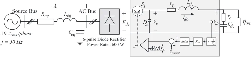
II. AC–DC POWERSYSTEMFEEDING ANIDEALCPL

108

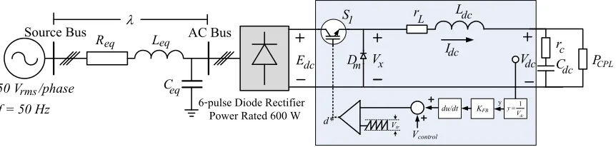
The ac–dc power system investigated in this study is depicted

109

in Fig. 1. An ac–dc power system including an uncontrolled

110

rectifier is considered in this paper because it is still widely

111

used in many applications. It consists of a balanced three-phase

112

voltage source, a transmission line represented byReq, Leq, and

113

Ceq, a six-pulse diode rectifier, dc-link filters represented by

114

rL, Ldc, rc, andCdc, and an ideal CPL represented by a

depen-115

dent current source. The parameters of the system in Fig. 1 are

116

given in Table I. Note that the inductance value has been chosen

117

in order for stability to occur at a power level that is able to be

118

verified experimentally.

119

It is known that CPLs can degrade the stability of their feeder

120

systems via the dc-link filter [3]–[5]. Many research works have

121

already presented how to predict unstable operation using a

122

mathematical model of the system. For three-phase systems with

123

six-pulse diode rectifiers, the DQ method [6]–[8] can be applied

124

in order to analyze the three-phase rectifier circuit and obtain

125

a dynamic model suitable for stability study. The eigenvalue

126

theorem [8] can then be applied to the linearized model for

127

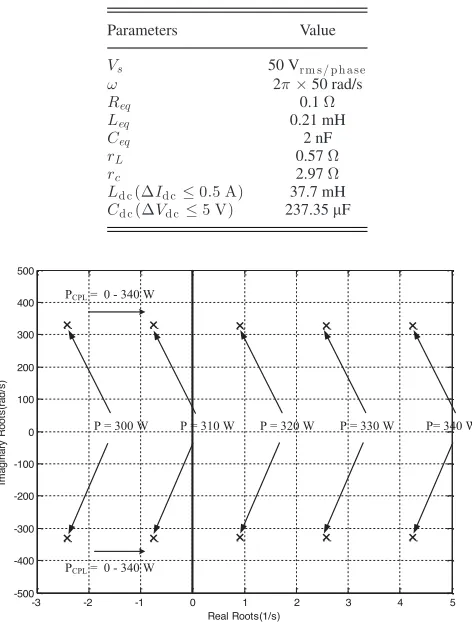
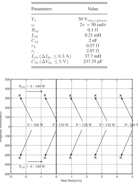
TABLE I

PARAMETERS OF THESYSTEM INFIG. 1

Parameters Value

Vs 50 Vrm s/p h a se

ω 2π×50 rad/s

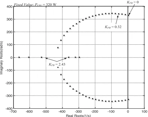
Req 0.1Ω

Leq 0.21 mH

Ceq 2 nF

rL 0.57Ω

rc 2.97Ω

[image:2.594.312.548.89.400.2]

Ld c(ΔId c≤0.5 A) 37.7 mH Cd c(ΔVd c≤5 V) 237.35µF

Fig. 2. Eigenvalue plot of the system before applied the proposed mitigation technique.

stability analysis. Based on the procedure in [9], the eigenvalue 128

plot of the system shown in Fig. 1, with the parameters in 129

Table I, is depicted in Fig. 2. It can be seen from Fig. 2 that 130

the system will be unstable when the value of PCPL reaches 131

320 W. In this paper, it will be shown that as a result of the 132

techniques used, the ac–dc system shown in Fig. 1 can provide 133

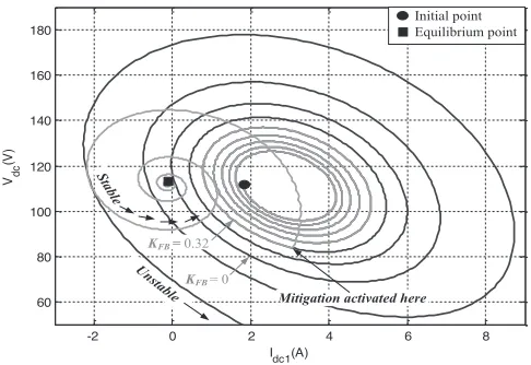
power exceeding 320 W, in this case up to 600 W (rated power), 134

without instability occurring. The details of the technique used 135

for the stabilization of the uncontrolled rectifier based ac–dc 136

power system will be explained in Section III. Moreover, the 137

novel adaptive stabilization for ac–dc power systems feeding 138

the CPLs is also explained. 139

III. LOOP-CANCELATIONSTABILIZATION OF ANAC–DC 140

POWERSYSTEMFEEDING ANIDEALCPL 141

Within this section, the new methodology for the application 142

of the loop-cancelation technique to uncontrolled rectifier based 143

ac–dc converters will be detailed. The established ac–dc con- 144

verters will be detailed. The established ac–dc power system, 145

on which this study is based, is shown in Fig. 1. The newly 146

proposed ac–dc power system, including the loop-cancelation 147

technique, is depicted in Fig. 3. An ideal CPL is considered ini- 148

tially in order to facilitate the calculation of the adaptable gain, 149

(3)

[image:3.594.82.513.69.172.2]

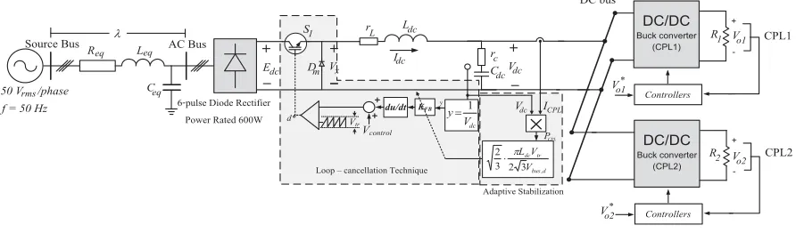
Fig. 3. AC–DC power system with the loop-cancelation technique.

Within dc–dc converters, the control of output dc voltage is

151

a natural feature. The loop-cancelation method [12] can

there-152

fore be conveniently applied to introduce a corrective action by

153

adjusting the converter duty cycle. In contrast, the ac–dc power

154

system in this study employs an uncontrolled rectifier in which

155

the output voltage cannot be adjusted and is defined by the ac

156

voltage magnitude only. Therefore, this study proposes a new

157

approach by introducing into the dc link a controlled switchS1

158

to both control the output voltage and introduce the proposed

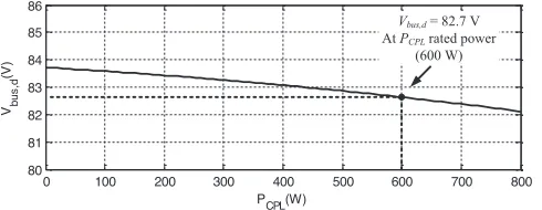
159

loop-cancelation technique. Only switchS1 and diodeDm are

160

added into the system, whereasrL, Ldc, rc, andCdc are the

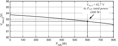
ex-161

isting dc-link filter of the rectifier circuit. Therefore, the effect

162

ofS1andDmon the overall system power loss and cost is very

163

small. The duty cycled∗is used to control the switchS1.d∗can

164

be calculated using

165

d∗= 1 Vtr

Vcontrol+KFB d

dt 1 Vdc (1)

whereVtris the amplitude of a triangular signal that can be set

166

by the user. Based on the loop-cancelation technique reported

167

in [12] for dc–dc converters, it is known that the feedback gain

168

KFBis a vital parameter that enables the designer to determine

169

the characteristic of output dc-link filter damping. Moreover, if

170

the designer can determine the appropriate value forKFB, the

171

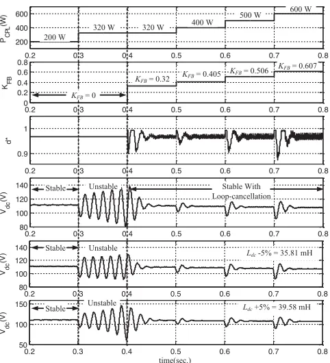
desired time-domain response can be obtained and the

destabi-172

lizing effect can be completely eliminated.

173

First, for the proposed uncontrolled rectifier based ac–dc

174

power system, the mathematical model will be derived. From

175

this, the equation for calculatingKFB can be obtained. As

de-176

tailed in previous publications [6]–[10], feeder systems with

177

three-phase rectifiers can be analyzed using the DQ method,

178

while the behavior of S1 can be eliminated by using the

179

generalized state-space averaging (GSSA) method [6]. The

180

equivalent circuit of the system in Fig. 3, represented in the

181

dq-frame, is shown in Fig. 4. After applying the DQ method, 182

the three-phase diode rectifier can be treated as a transformer

183

in the dq-frame [10]. The GSSA is then used to eliminate the

184

switching behavior of S1. Applying Kirchhoff’s voltage law

185

and Kirchhoff’s current law to the circuit shown in Fig. 4,

186

withd∗given by (1), the mathematical model of the proposed

187

ac–dc power system under continuous conduction mode,

us-188

ing the loop-cancelation technique, is defined by the following

189 equation: 190 ⎧ ⎪ ⎪ ⎪ ⎪ ⎪ ⎪ ⎪ ⎪ ⎪ ⎪ ⎪ ⎪ ⎪ ⎪ ⎪ ⎪ ⎪ ⎪ ⎪ ⎨ ⎪ ⎪ ⎪ ⎪ ⎪ ⎪ ⎪ ⎪ ⎪ ⎪ ⎪ ⎪ ⎪ ⎪ ⎪ ⎪ ⎪ ⎪ ⎪ ⎩ •

Ids =−R_Leq_eqIds+ωIq s−_L1_eqVbus,d+_L1_eqVsd

•

Iq s=−ωIds−R_Leq_eqIq s−_L1_eqVbus,q+_L1_eqVsq

•

Vbus,d =_C1_eqIds+ωVbus,q

−3 2 ·

2√3Vt r

π Ceq Vcontrol+KF Bd td V1_{d c}

_I_dc

•

Vbus,q =−ωVbus,d+_C1_eqIq s

•

Idc =

3 2 · 2

√ 3Vcontrol

π Ld cVt r Vbus,d−

(rμ+rL+rc)

Ld c Idc− 1

Ld cVdc

+rcPC P L

Ld cVd c +

3 2 · 2

√ 3

π Ld cCd c

KF BVb u s, d

Vt r

d dt V1d c

•

Vdc = _C1_{d c} Idc−_CP_{d c}C P L_V_{d c}

.

(2)

191

A new variableIdc1, as given by (3), can be used to simplify 192

the system model 193

•

Idc1= •

Idc−

3 2 .

2√3 πLdc

KFBVbus,d

Vtr d dt 1 Vdc . (3)

Hence, (2) can be written as the following equation: 194 ⎧ ⎪ ⎪ ⎪ ⎪ ⎪ ⎪ ⎪ ⎪ ⎪ ⎪ ⎪ ⎪ ⎪ ⎪ ⎪ ⎪ ⎪ ⎪ ⎨ ⎪ ⎪ ⎪ ⎪ ⎪ ⎪ ⎪ ⎪ ⎪ ⎪ ⎪ ⎪ ⎪ ⎪ ⎪ ⎪ ⎪ ⎪ ⎩ •

•

Iq s=−ωIds−R_L_eqeqIq s−_L1_eqVbus,q+_L1_eqVsq

•

Vbus,d =C1eqIds+ωVbus,q −

3 2 · 2

√ 3Vt r

π CeqVcontrolIdc1

+ 18KF B

π2_C

eqLd cVcontrol

Vb u s, d

Vd c •

•

Idc1 =

3 2 · 2

√ 3Vcontrol

(rμ+rL+rc)

Ld c Idc1− 1

Ld cVdc −3

2 ·

2√3(rμ+rL+rc)KF B

π L2 d cVt r

Vb u s, d

Vd c +

rcPC P L

Ld cVd c •

Vdc = _C1_{d c} Idc1−_CP_{d c}C P L_V_{d c} +

3 2 · 2

√ 3

π Ld cCd c

KF B

Vd cVt r

Vbus,d

.

(4) It can be seen from (4) thatKFB is presented in the system 195 model. The effect of KFB can be assessed via a plot of the 196 dominant eigenvalues. These eigenvalues were calculated from 197

the linearization of (4). The system parameters for this plot are 198

given in Table I withVcontrol=2.9 V, Vtr=3 V, andPCPL = 199

320 W. The dominant eigenvalue plot when gainKFBis varied 200

from 0 to 2.45 is shown in Fig. 5. The plot within Fig. 5 can 201

be used to determine the best value ofKFB to avoid unstable 202

(4)

[image:4.594.107.491.72.204.2] [image:4.594.308.552.242.409.2]

Fig. 4. Equivalent circuit of the ac–dc power system with the loop-cancelation technique in the dq-frame.

Fig. 5. Eigenvalue plot for the ac–dc power system with the loop-cancelation technique by varyingKF B.

the location of dominant poles. However, the plot will change

204

whenPCPL changes. Therefore, the appropriate value ofKFB

205

to mitigate the instability problem should be adapted according

206

to the variation ofPCPL.

207

Large-signal stability analysis of the example system is shown

208

in Fig. 6 via a phase-plane plot. Initially,PCPLis set at 200 W.

209

Subsequently,PCPLis increased to 320 W. IfKFB = 0(without

210

mitigation), huge oscillation occurs, as shown by the blue line

211

in Fig. 6. Conversely, if the proposed mitigation is applied with

212

KFB =0.32, the system can regain stability as depicted by the

213

green line in Fig. 6. It can be seen from Figs. 5 and 6 that there

214

is good agreement between the eigenvalue plot and phase-plane

215

plot. Both methodologies confirm that stability is achieved when

216

KFB =0.32. However,KFB = 0.32is forPCPL =320 W. If

217

PCPL is increased, KFB should be increased to ensure that

218

the system maintains stable operation. Hence, KFB must be

219

adaptable depending on the level ofPCPL. In this paper, a novel

220

equation is used to calculate the adaptable gain. The derivation

221

of this equation is detailed as follows.

222

Considering only the characteristics of output dc-link filter

223

damping, the differential equationsI˙dc1andV˙dcin (4) will now

224

be analyzed. It can be seen that the nonlinear terms ofKFBoccur

[image:4.594.48.289.246.437.2]

225

Fig. 6. Phase-plane plot of the ac–dc power system.

in both I˙dc1 and V˙dc. However, normally (rμ+rL+r)<< 226

Ldc, therefore only the nonlinear terms ofKFB withinV˙dc are 227

required. If parameterP1is defined as 228

P1 =

3 2

2√3Vbus,d

πLdcCdcVtr

KFB− 1 2√3.

2 3

πLdcVtrPCPL

Vbus,d

(5) thenV˙dcin (4) can be written as 229

˙ Vdc = 1

Cdc Idc1+

P1

Vdc.

(6)

According to (6), ifP1= 0, the nonlinear termP1/Vdc can 230

be canceled. Therefore,KFB in order to guarantee thatP1 = 0 231

can be defined from (5). The adaptable value ofKFB can then 232 be calculated in order to stabilize the system according to 233

KFB = 1 2√3.

2 3

πLdcVtrPCPL

Vbus,d .

(7)

The final system, with adaptive stabilization based on the 234

loop-cancelation technique, is shown in Fig. 7. It can be seen 235

in Fig. 7 that the loop cancelation gainKFBis calculated as in 236

(7).KFB will be adapted depending on the value of the system 237

operating point defined byPCPL. From (7), the adaptableKFB 238

(5)

[image:5.594.88.509.67.197.2] [image:5.594.43.288.243.338.2]

Fig. 7. System with the adaptive stabilization based on the loop-cancelation technique.

Fig. 8. Vb u s,dvalues forPC P Lwhen varied from 0 to 800 W.

example system used in this paper,Ldc =37.7 mH; however,

240

in other systems this can be determined by the measurement or

241

identified by artificial intelligence techniques [31]. The value of

242

Vbus,dcan be determined by using the power flow equation [9]

243

based on the ac side. TheVbus,d values of the example system

244

in Fig. 1, when thePCPL is varied from 0 to 800 W (the rated

245

power is 600 W), are shown in Fig. 8.

246

According to Fig. 8 at the rated power of 600 W, the value

247

ofVbus,dfor the example system is 82.7 V. It can be seen from

248

Fig. 8 that the higher the value ofPCPL, the lower the value of

249

Vbus,d. This in turn results in a higher value ofKFB. Finally,

250

PCPLcan be determined according to (8). The required values of

251

ICPLandVdccan be obtained from current and voltage sensors,

252

respectively

253

PCPL =VdcICPL. (8)

To ensure that condition (7) can provide the appropriate value

254

ofKFB, a phase-plane analysis of the system in Fig. 7 was

per-255

formed. The phase-plane plots forPCPL =400, 500, and 600 W

256

are shown in Fig. 9(a)–(c), respectively. It can be seen that if

257

thePCPL is increased, the value ofKFB is also automatically

258

increased based on (7). It can be seen from Fig. 9(a) that the

259

system without the proposed mitigation technique(KFB = 0)

260

is unstable; this is represented by the blue line. However, when

261

the mitigation is activated att= 0.1s, withKFB = 0.405, the

262

system settles to a new stable operating point. This stabilization

263

trajectory is represented by the green line in Fig. 9(a). Similarly,

264

as shown in Fig. 9(b) and (c), the system withPCPL =500 W

265

and 600 W becomes stable withKFB = 0.506 and 0.607,

re-266

spectively. These analytical results, via phase-plane analysis,

267

Fig. 9. Phase-plane plots of the system with the proposed adaptive stabiliza-tion. (a)PC P L=400 W. (b)PC P L=500 W. (c)PC P L=600 W.

confirm that the adaptable KFB calculated from (7) ensures 268

stable operation. 269

Time-domain simulation results whenPCPL is varied from 270

[image:5.594.315.534.243.646.2]

(6)

[image:6.594.48.289.66.331.2]

Fig. 10. Time-domain simulation results with adaptive stabilization based on the loop-cancelation technique.

can be seen from Fig. 10 that the system is initially unstable

272

between 0.3 and 0.4 s whenKFB = 0. However, once the

loop-273

cancelation technique is activated at 0.4 s the system becomes

274

stable and remains stable under all subsequent values ofPCPL.

275

After 0.4 s, current and voltage sensors are used to continuously

276

monitor the value ofPCPLin order to recalculate the appropriate

277

KFB. This can be seen in Fig. 10. The duty cycle ofS1 is also

278

included in Fig. 10. This value cannot exceed one for practical

279

implementation. Hence, this limitation has already been added

280

in the simulation, as can be seen in Fig. 10. The simulation

281

results using the same value ofKFBforLdc−5% =35.81 mH

282

andLdc+ 5% =39.58 mH are also shown. It can be seen that

283

even thoughLdc is changed to 35.81 or 39.58 mH, the system

284

can remain stable by using theKFBcalculated from fixedLdc =

285

37.7 mH. It means that the parameter robustness of the proposed

286

control method does not affect the mitigation result.

287

IV. EXPERIMENTALVERIFICATION 288

It has been established in the previous sections that the

pro-289

posed ac–dc power system shown in Fig. 1 becomes unstable

290

whenPCPL is equal to 320 W. Adaptive loop cancelation has

291

been analytically proven to mitigate the instability, as shown

292

in Fig. 7. The simulation results shown in Fig. 10 have also

293

confirmed that the system is always stable with adaptableKFB.

294

In this section, experimental verification is reported in order to

295

support the proposed adaptive stabilization concept. The same

296

ac–dc system is used as shown in Fig. 7. However, within the

297

experimental rig, two parallel tightly controlled buck

convert-298

ers are used to represent the ideal CPL. More details on these

299

converters can be found in [9]. In addition, as the time-domain

300

simulation results presented in the previous section were per- 301

formed with an ideal CPL, they were repeated also using two 302

paralleled buck converters. A diagrammatic representation of 303

the ac–dc power system examined in this section, with the pro- 304

posed adaptive stabilization, is shown in Fig. 11. 305

The experimental rig is shown in Fig. 12. The MOSFET 306

IRFP250N and the diode MUR1560G were added into the sys- 307

tem to represent theS1 andDm, respectively. Moreover, the 308

low-pass filter was already embedded to eliminate the noise 309

generated from the derivative term. The bandwidth of the low- 310

pass filter is set equal to ten times the resonance frequency [12]. 311

In this paper, the resonance frequency is equal to 343.3 rad/s, 312

calculated from theLdc andCdc values shown in Table I. The 313

proposed adaptive stabilization, based on the loop-cancelation 314

technique, was implemented using an Atmaga1280 microcon- 315

troller with analog circuits. This is highlighted by the number 3 316

in Fig. 12. As for both controlled buck converters highlighted by 317

the number 5 and 7, a damping ratio(ζ)and a natural frequency 318

(ωn)for a voltage loop were set to 0.7 and 2π(400) rad/s, re- 319

spectively. For a current loop, these values were equal to 0.7 and 320

2π(4000) rad/s. Hence, following on these damping ratios and 321

natural frequencies,Kpv, Kiv, Kpi, andKii are equal to 0.05, 322

20, 0.6819, and 1948, respectively. In addition, the switching 323

frequencies for switch S1 and switches inside the controlled 324

buck converters were equal to 10 kHz. 325

Both the simulation model and the experimental rig were 326

subjected to the same test scenario. The resultingVdcwaveforms 327

are shown in Fig. 13. The test scenario can be summarized as 328

follows. 329

1) Initially, the total load power was set to 250 W; CPL1= 330

250 W, CPL2=0 W. 331

2) At t=0.11 s, an additional load of 24.2 W is introduced 332

by the second converter CPL2, as a result the total CPL 333

becomes 274.2 W. From the experimental results, it can 334

be seen that the system response is now poorly damped 335

indicating that the stability margin is approaching. The 336

simulation also shows a very oscillatory response, how- 337

ever of a much smaller magnitude. This discrepancy can 338

be explained by unaccounted parasitic effects and mod- 339

eling assumptions. Hence, both the simulation model and 340

the experimental setup indicate that the system is close to 341

instability. 342

3) At t=0.43 s, CPL2 is increased to 80 W. As predicted 343

from the analytical analysis presented in the previous sec- 344

tion, at a total load power of 330 W, the system becomes 345

unstable. It can be seen from Fig. 13 that in both simula- 346

tion and experimental results, the dc voltage exhibits an 347

expanding oscillatory behavior. 348

4) At t=1.05 s, the proposed algorithm is activated and the 349

system stabilizes. 350

5) At t=1.15 s, the load power is further increased (CPL 351

total power becomes 380 W). The system maintains stable 352

operation due to the stabilizing effect of proposed adaptive 353

stabilization technique. 354

6) Finally, to confirm that the system maintains stability even 355

with higher loads, two further CPL step increases are 356

(7)

[image:7.594.73.519.71.202.2] [image:7.594.43.285.241.345.2]

Fig. 11. AC–DC power system with the proposed adaptive stabilization feeding paralleled controlled buck converters.

[image:7.594.43.285.394.532.2]

Fig. 12. Testing rig based on the system in Fig. 11.

Fig. 13. (a) Simulation and (b) experimental results.

and at t =1.38 s (600 W total). It is clearly seen from

358

Fig. 13 that the dc bus voltage responses are stable and

359

that the voltage drops at each load step according to the

360

system’s internal resistance.

361

Overall, it can be concluded that there is a very good match

362

between the simulation and experiment results during the test

363

scenario. The capability of the system to return to stable

opera-364

tion using the proposed technique is clearly shown. Furthermore,

365

once the proposed mitigation has been activated, the results in

366

Fig. 13 confirm that the system is always stable even when the

367

total CPL is equal to 600 W (the rated power of feeder

sys-368

tem). The experimental results confirm that the proposed

adap-369

tive stabilization algorithm, based on the loop-cancelation

tech-370

nique, fully mitigates the ac–dc feeder system instability caused

371

by CPLs. In addition, Fig. 13 validates the developed system 372

model and the assumptions made during the development of this 373

effective technique. 374

V. CONCLUSION 375

In this paper, adaptive stabilization of an uncontrolled recti- 376

fier based ac–dc converter has been introduced. The proposed 377

mitigation technique has been used to eliminate the destabi- 378

lizing effect of CPLs. As a result, the ac–dc feeder system is 379

always stable for any level of CPL. The theoretical results from 380

the eigenvalue theorem and the phase-plane analysis confirm 381

that the uncontrolled rectifier based ac–dc power system, with 382

the proposed adaptive stabilization, is always stable. Moreover, 383

simulations and experimental results have been used to verify 384

the theoretical results. Agreement between theoretical, simula- 385

tion, and experimental results has been shown. The proposed 386

adaptive mitigation is therefore a very powerful and flexible 387

technique, which can be used to guarantee the stable opera- 388

tion of uncontrolled rectifier based ac–dc feeder systems when 389

supplying CPLs. 390

REFERENCES 391

[1] V. Grigore, J. Hatonen, J. Kyyra, and T. Suntio, “Dynamics of a buck 392 converter with a constant power load,” in Proc. IEEE 29th Power Electron. 393

Spec. Conf., Fukuoka, Japan, May 1998, pp. 72–78. 394

[2] A. Emadi, M. Ehsani, and J. M. Miller, Vehicular Electric Power Systems: 395

Land, Sea, Air, and Space Vehicle. New York, NY, USA: Marcel Dekker, 396

2003. 397

[3] R. D. Middlebrook, “Input filter consideration in design and application 398 of switching regulators,” in Proc. Conf. Record IEEE IAS Annu. Meeting, 399

1967, pp. 366–382. 400

[4] A. M. Rahimi and A. Emadi, “An analytical investigation of DC/DC 401 power electronic converters with constant power loads in vehicular power 402 systems,” IEEE Trans. Veh. Technol., vol. 58, no. 6, pp. 2689–2702, 403

Jul. 2009. 404

[5] A. Emadi, A. Khaligh, C. H. Rivetta, and G. A. Williamson, “Constant 405 power loads and negative impedance instability in automotive systems: 406 Definition, modeling, stability, and control of power electronic con- 407 verters and motor drives,” IEEE Trans. Veh. Technol., vol. 55, no. 4, 408

pp. 1112–1125, Jul. 2006. 409

[6] A. Emadi, “Modeling of power electronic loads in AC distribution systems 410 using the generalized state-space averaging method,” IEEE Trans. Ind. 411

Electron., vol. 51, no. 5, pp. 992–1000, Oct. 2004. 412

(8)

[8] K.-N. Areerak, T. Wu, S. V. Bozhko, G. M. Asher, and D. W. P. Thomas, 417

“Aircraft power system stability study including effect of voltage control 418

and actuators dynamic,” IEEE Trans. Aerosp. Electron. Syst., vol. 47, 419

no. 7, pp. 2574–2589, Oct. 2011. 420

[9] T. Sopapirm, K.-N. Areerak, and K.-L. Areerak, “Stability analysis of 421

AC distribution system with six-pulse diode rectifier and multi-converter 422

power electronic loads,” Int. Rev. Elect. Eng., vol. 6, no. 7, pt. A, 423

pp. 2919–2928, Nov./Dec. 2011. 424

[10] K.-N. Areerak, S. V. Bozhko, G. M. Asher, L. De lillo, and D. W. P. 425

Thomas, “Stability study for a hybrid AC-DC more-electric aircraft power 426

system,” IEEE Trans. Aerosp. Electron. Syst., vol. 48, no. 1, pp. 329–347, 427

Jan. 2012. 428

[11] A. M. Rahimi and A. Emadi, “Active damping in dc/dc power elec-429

tronic converters: A novel method to overcome the problems of constant 430

power loads,” IEEE Trans. Ind. Electron., vol. 56, no. 5, pp. 1428–1439, 431

Feb. 2009. 432

[12] A. M. Rahimi, G. A. Williamson, and A. Emadi, “Loop-cancellation 433

technique: A novel nonlinear feedback to overcome the destabilizing ef-434

fect of constant-power loads,” IEEE Trans. Veh. Technol., vol. 59, no. 2, 435

pp. 650–661, Feb. 2010. 436

[13] M. Cespedes, L. Xing, and J. Sun, “Constant-power loads system sta-437

bilization by passive damping,” IEEE Trans. Power Electron., vol. 26, 438

no. 7, pp. 1832–1836, Jul. 2011. 439

[14] X. N. Zhang, D. M. Vilathgamuwa, K. J. Tseng, B. S. Bhangu, and 440

G. Chandana, “A loop cancellation based active damping solution for con-441

stant power instability in vehicular power systems,” in Proc. 2012 IEEE 442

Energy Convers. Congr. Expo., Raleigh, NC, USA, 2012, pp. 1182–1187.

443

[15] Y. Li, L. R. Vannorsdel, A. J. Zirger, M. Norris, and D. Makismovic, 444

“Current mod control for boost converters with constant power loads,” 445

IEEE Trans. Circuits Syst. I, Reg. Papers, vol. 59, no. 1, pp. 198–206,

446

Jan. 2012. 447

[16] A. A. A. Radwan and Y. R. Mohamed, “Linear active stabilization of 448

converter-dominated dc microgrid,” IEEE Trans. Smart Grid, vol. 3, 449

no. 1, pp. 203–216, Mar. 2012. 450

[17] A. A. A. Radwan and Y. Mohamed, “Assessment and mitigation of inter-451

action dynamics in hybrid ac/dc distribution generation systems,” IEEE 452

Trans. Smart Grid, vol. 3, no. 3, pp. 1382–1393, Sep. 2012.

453

[18] R. Ahmadi and W. Ferdowsi, “Improving the performance of a line reg-454

ulating converter in a converter-dominated dc microgrid system,” IEEE 455

Trans. Smart Grid, vol. 5, no. 5, pp. 2553–2563, Sep. 2014.

456

[19] M. Wu and D. D. Lu, “A novel stabilization method of LC input filter 457

with constant power loads without load performance compromise in dc 458

microgrid,” IEEE Trans. Ind. Electron., vol. 62, no. 7, pp. 4552–4562, 459

Jul. 2015. 460

[20] H. Mahmoudi, M. Aleenejad, and R. Ahmadi, “A new modulated model 461

predictive control method for mitigation of effects of constant power 462

loads,” in Proc. Power Energy Conf. Illinois, 2016, pp. 1–5. 463

[21] Y. R. Mohamed, A. A. A. Radwan, and T. Lee, “Decoupled refer-464

ence voltage-based active dc-link stabilization for PMSM drives with 465

tight-speed regulation,” IEEE Trans. Ind. Electron., vol. 59, no. 12, 466

pp. 4523–4536, Dec. 2012. 467

[22] P. Magne, B. Nahid-Mobarakeh, and S. Pierfederici, “General active global 468

stabilization of multiloads dc-power networks,” IEEE Trans. Power Elec-469

tron., vol. 27, no. 4, pp. 1788–1798, Apr. 2012.

470

[23] P. Magne, D. Marx, B. Nahid-Mobarakeh, and S. Pierfederici, “Large-471

signal stabilization of a dc-link supplying a constant power load using a 472

virtual capacitor: Impact on the domain of attraction,” IEEE Trans. Ind. 473

Appl., vol. 48, no. 3, pp. 878–887, May/Jun. 2012.

474

[24] P. Magne, B. Nahid-Mobarakeh, and S. Pierfederici, “Active stabilization 475

of dc microgrids without remote sensors for more electric aircraft,” IEEE 476

Trans. Ind. Appl., vol. 49, no. 5, pp. 2352–2360, Sep./Oct. 2013.

477

[25] W. J. Lee and S. K. Sul, “DC-link voltage stabilization for reduced DC-link 478

capacitor inverter,” IEEE Trans. Ind. Appl., vol. 50, no. 1, pp. 404–414, 479

Jan./Feb. 2014. 480

[26] P. Magne, B. Nahid-Mobarakeh, and S. Pierfederici, “Dynamic consid-481

eration of dc microgrids with constant power loads and active damping 482

system a design method for fault-tolerant stabilizing system,” IEEE J. 483

Emerg. Sel. Topics Power Electron., vol. 2, no. 3, pp. 562–570, Sep. 2014.

484

[27] H. Mosskull, “Optimal stabilization of constant power loads with input 485

LC-filters,” Control Eng. Pract., vol. 27, pp. 61–63, 2014. 486

[28] K. Inoue, T. Kato, M. Inoue, Y. Moriyama, and K. Nishii, “An oscillation 487

suppression method of a dc-bus supply system with a constant power load 488

and a LC filter,” in Proc. 2012 IEEE 13th Workshop Control Model. Power 489

Electron., 2012, pp. 1–4.

490

[29] M. S. Carmeli, D. Forlani, S. Grillo, R. Pinetti, E. Ragaini, and E. Tironi, 491 “A stabilization method for dc networks with constant-power loads,” in 492

Proc. 2012 IEEE 36th Int. Energy Conf. Exhib., 2012, pp. 617–622. 493

[30] O. Pizniur, Z. Shan, and J. Jatskevich, “Ensuring dynamic stability of 494 constant power loads in dc telecom power systems and data centers using 495 active damping,” in Proc. 2014 IEEE 36th Int. Telecommun. Energy Conf., 496

2012, pp. 1–8. 497

[31] T. Sopaprim, K.-N. Areerak, and K.-L. Areerak, “The identification of AC- 498 DC power system parameter using an adaptive tabu search technique,” Int. 499

Rev. Elect. Eng., vol. 7, no. 4, pp. 4655–4662, Jul./Aug. 2012. 500

Kongpan Areerak received the B.Eng. and M.Eng. 501 degrees from Suranaree University of Technology 502 (SUT), Nakhon Ratchasima, Thailand, in 2000 and 503 2001, respectively, and the Ph.D. degree from the 504 University of Nottingham, Nottingham, U.K., in 505 2009, all in electrical engineering. 506 In 2002, he was a Lecturer with the Electrical and 507 Electronic Department, Rangsit University, Lak Hok, 508 Thailand. Since 2003, he has been a Lecturer with 509 the School of Electrical Engineering, SUT, and since 510 2015 he has been an Associate Professor in electrical 511 engineering. His research interests include system identifications, artificial in- 512 telligence applications, stability analysis of power systems with constant power 513 loads, modeling and control of power electronic based systems, and control 514

theory. 515

516

Theppanom Sopapirm was born in Saraburi, 517 Thailand, in 1988. He received the B.Eng., M.Eng., 518 Ph.D. degrees in electrical engineering from Surana- 519 ree University of Technology, Nakhon Ratchasima, 520 Thailand, in 2009, 2011, and 2017, respectively. 521 His research interests include stability analysis, 522 modeling of power electronic systems, digital con- 523 trol, FPGA, and AI applications. 524 525

Serhiy Bozhko received the M.Sc. (Hons.) and Ph.D. 526 degrees in electromechanical systems from the Na- 527 tional Technical University of Ukraine, Kyiv City, 528 Ukraine, in 1987 and 1994, respectively. 529 Since 2000, he has been with the Power Electron- 530 ics, Machines and Controls Research Group, Univer- 531 sity of Nottingham, Nottingham, U.K., where he is 532 currently a Professor with the Aircraft Electric Power 533 Systems Innovations Laboratory. He is leading sev- 534 eral EU- and industry-funded projects dealing with 535 the electric power systems for aerospace applications. 536 His research interests include their control, power quality and stability issues, 537 power management and optimization, as well as advanced modeling and simu- 538

lations methods. 539

540

Christopher Ian Hill (M’08) received the M.Eng. 541 and Ph.D. degrees from The University of Not- 542 tingham, Nottingham, U.K., in 2004 and 2014, 543

respectively. 544

In March 2012, he joined the Power Electronics, 545 Machines and Control Research Group, University of 546 Nottingham, as a Research Fellow. In 2017, he was 547 promoted to Senior Research Fellow at The Univer- 548 sity of Nottingham and currently leads several Eu- 549 ropean projects totaling more than€2 million. His 550 current research interests include hybrid and fully 551 electric aircraft; future aircraft electrical power system design, sizing, and op- 552 timization; onboard energy management and optimization; superconducting 553 electrical power systems; advanced multilevel modeling; and advanced fault 554

and loss modeling. 555

(9)

Apichai Suyapan was born in Chiang Mai, 557

Thailand, in 1991. He received the B.Eng. and M.Eng. 558

degrees in electrical engineering, in 2013 and 2016, 559

respectively, from Suranaree University of Technol-560

ogy, Nakhon Ratchasima, Thailand, where he is cur-561

rently working toward the Ph.D. degree in electrical 562

engineering. 563

His research interests include stability analysis of 564

power systems with constant power loads, modeling 565

and control of power electronic based systems, and 566

control theory. 567

568

Kongpol Areerak received the B.Eng., M.Eng., 569 and Ph.D. degrees in electrical engineering from 570 Suranaree University of Technology (SUT), Nakhon 571 Ratchasima, Thailand, in 2000, 2003, and 2007, 572

respectively. 573

Since 2007, he has been a Lecturer and Head of 574 the Power Quality Research Unit with the School 575 of Electrical Engineering, SUT. In 2009, he was an 576 Assistant Professor in electrical engineering. His re- 577 search interests include active power filters, harmonic 578 elimination, AI applications, motor drives, and intel- 579

ligence control system. 580

(10)