C
2015. The American Astronomical Society. All rights reserved.
IGM CONSTRAINTS FROM THE SDSS-III
/
BOSS DR9 Ly
α
FOREST TRANSMISSION
PROBABILITY DISTRIBUTION FUNCTION
Khee-Gan Lee1,2, Joseph F. Hennawi1, David N. Spergel2, David H. Weinberg3, David W. Hogg4, Matteo Viel5,6, James S. Bolton7, Stephen Bailey8, Matthew M. Pieri9, William Carithers8,
David J. Schlegel8, Britt Lundgren10, Nathalie Palanque-Delabrouille11, Nao Suzuki12, Donald P. Schneider13,14, and Christophe Y`eche11
1Max Planck Institute for Astronomy, K¨onigstuhl 17, D-69117 Heidelberg, Germany;[email protected] 2Department of Astrophysical Sciences, Princeton University, Princeton, NJ 08544, USA
3Department of Astronomy and Center for Cosmology and Astro-Particle Physics, Ohio State University, Columbus, OH 43210, USA 4Center for Cosmology and Particle Physics, New York University, 4 Washington Place, Meyer Hall of Physics, New York, NY 10003, USA
5INAF, Osservatorio Astronomico di Trieste, Via G. B. Tiepolo 11, I-34131 Trieste, Italy 6INFN/National Institute for Nuclear Physics, Via Valerio 2, I-34127 Trieste, Italy
7School of Physics and Astronomy, University of Nottingham, University Park, Nottingham NG7 2RD, UK 8E.O. Lawrence Berkeley National Lab, 1 Cyclotron Road, Berkeley, CA 94720, USA
9Institute of Cosmology & Gravitation, University of Portsmouth, Dennis Sciama Building, Portsmouth PO1 3FX, UK 10Department of Astronomy, University of Wisconsin, Madison, WI 53706, USA
11CEA, Centre de Saclay, Irfu/SPP, F-91191 Gif-sur-Yvette, France
12Kavli Institute for the Physics and Mathematics of the Universe (IPMU), The University of Tokyo, Kashiwano-ha 5-1-5, Kashiwa-shi, Chiba, Japan 13Department of Astronomy and Astrophysics, The Pennsylvania State University, University Park, PA 16802, USA
14Institute for Gravitation and the Cosmos, The Pennsylvania State University, University Park, PA 16802, USA
Received 2014 May 5; accepted 2014 December 4; published 2015 January 29
ABSTRACT
The Lyαforest transmission probability distribution function (PDF) is an established probe of the intergalactic medium (IGM) astrophysics, especially the temperature–density relationship of the IGM. We measure the transmission PDF from 3393 Baryon Oscillations Spectroscopic Survey (BOSS) quasars from Sloan Digital Sky Survey Data Release 9, and compare with mock spectra that include careful modeling of the noise, continuum, and astrophysical uncertainties. The BOSS transmission PDFs, measured at z = [2.3,2.6,3.0], are compared with PDFs created from mock spectra drawn from a suite of hydrodynamical simulations that sample the IGM temperature–density relationship,γ, and temperature at mean density,T0, whereT(Δ)=T0Δγ−1. We find that a significant population of partial Lyman-limit systems (LLSs) with a column-density distribution slope ofβpLLS∼ −2
are required to explain the data at the low-transmission end of transmission PDF, while uncertainties in the mean
Lyαforest transmission affect the high-transmission end. After modeling the LLSs and marginalizing over mean
transmission uncertainties, we find that γ =1.6 best describes the data over our entire redshift range, although
constraints on T0 are affected by systematic uncertainties. Within our model framework, isothermal or inverted
temperature–density relationships (γ1) are disfavored at a significance of over 4σ, although this could be somewhat weakened by cosmological and astrophysical uncertainties that we did not model.
Key words: intergalactic medium – large-scale structure of universe – methods: data analysis – quasars: absorption lines – quasars: emission lines – techniques: spectroscopic
1. INTRODUCTION
Remarkably soon after the discovery of the first high-redshift (zqso 2) quasars (Schmidt 1965), Gunn & Peterson (1965) realized that the amount of resonant Lyman-α(Lyα) scattering off neutral hydrogen structures observed in the spectra of these quasars could be used to constrain the state of the intergalactic medium (IGM) at high-redshifts: they deduced that the hydrogen in the IGM had to be highly photo-ionized (neutral fractions of
nHi/nH<10−4) and hot (temperatures,T >104K).
Lynds (1971) then discovered that this Lyαabsorption could be separated into discrete absorption lines, i.e., the Lyα“forest.” Over the next two decades, it was recognized that the individual Lyα forest lines have Voigt absorption profiles corresponding
to Doppler-broadened systems withT ∼1−3×10⁴ K (see,
e.g., Rauch et al.1992; Ricotti et al.2000; Schaye et al.2000; McDonald et al.2001; Tytler et al.2004; Lidz et al.2010; Becker et al.2011) and neutral column densities ofN∼1013–1017cm−2
(Petitjean et al.1993; Penton et al.2000; Janknecht et al.2006;
Rudie et al.2013), and increasingly precise measurements of
mean Lyα forest transmission have been carried out (Theuns
et al.2002; Bernardi et al.2003; Faucher-Gigu`ere et al.2008; Becker et al.2013). However, the exact physical nature of these
absorbers was unclear for many years (see Rauch1998, for a
historical review of the field).
Beginning in the 1990s, detailed hydrodynamical simulations of the IGM led to the current physical picture of the Lyαforest arising from baryons in the IGM, which trace fluctuations in the dark matter (DM) field induced by gravitational collapse, in ion-ization balance with a uniform ultraviolet ionizing background (see, e.g., Cen et al.1994; Miralda-Escud´e et al. 1996; Croft et al.1998; Dav´e et al.1999; Theuns et al.1998). A physically motivated analytic description of this picture is the fluctuat-ing Gunn–Peterson approximation (Croft et al.1998; Hui et al. 1997), in which the Lyαoptical depth,τ, scales with underlying matter density,ρ, through a polynomial relationship:
τ ∝ T −0.7 Γ Δ2 ∝
T0−0.7 Γ Δ2−0
.7(γ−1), (1)
whereΓis the background photoionization rate, andΔ≡ρ/ρ
a dramatic improvement in the statistical power available to Lyαforest studies: McDonald et al. (2006) measured the
one-dimensional (1D) Lyαforest transmission power spectrum from
≈3000 SDSS quasar sightlines. This measurement was used to
place significant constraints on cosmological parameters and large-scale structure (see, e.g., McDonald et al.2005b; Seljak et al.2005; Viel & Haehnelt2006).
The McDonald et al. (2006) quasar sample, which in its
time represented a∼100 increase in sample size over previous data sets, is superseded by the Baryon Oscillations Sky Survey (BOSS; part of SDSS-III; Eisenstein et al.2011; Dawson et al. 2013) quasar survey. This spectroscopic survey, which operated between fall 2009 and spring 2014, is aimed at taking spectra
of ∼150,000 zqso 2.2 quasars (Dawson et al. 2013) with
the goal of constraining dark energy atz >2 using transverse correlations of Lyα forest absorption (see, e.g., Slosar et al. 2011) to measure the baryon acoustic oscillation (BAO) scale.15 At time of writing, the full BOSS survey is complete, with
∼170,000 high-redshift quasars observed, although this paper
is based on the earlier sample of∼50,000 BOSS quasars from
SDSS Data Release 9 (DR9; Ahn et al.2012; Pˆaris et al.2012; Lee et al.2013).
The quality of the individual BOSS Lyαforest spectra might appear at first glance inadequate for studying the astrophysics of the IGM, that have to date been carried out largely with high-resolution, high-signal-to-noise ratio (S/N) spectra: the typical BOSS spectrum has S/N∼2 pixel−1,16since the BAO analysis
is optimized with large numbers of low S/N sightlines, densely
sampled on the sky (McDonald & Eisenstein2007; McQuinn
& White2011). It is therefore interesting to ask whether it is possible to model the various instrumental and astrophysical
effects seen in the BOSS Lyα forest spectra, to sufficient
accuracy level to exploit the unprecedented statistical power. In this paper, we will measure the probability distribution function (PDF) of the Lyαforest transmission,F ≡exp(−τ), from BOSS. This one-point statistic, which was first studied by Jenkins & Ostriker (1991), is sensitive to astrophysical parameters such as the amplitude of matter fluctuations and
the thermal history of the IGM. However, the transmission17
PDF is also highly sensitive to effects such as pixel noise level, resolution of the spectra, and systematic uncertainties
15 There is also a simultaneous effort to observe∼1.5 million luminous red galaxies, to measure the BAO atz∼0.5. See, e.g., Anderson et al. (2014). 16 All spectral signal-to-noise ratios quoted in this paper are per 69 km s−1 SDSS/BOSS pixel unless noted otherwise.
17 The Lyαforest transmitted flux fraction is sometimes also referred to as “flux” in the literature; but we do however use the variableFto refer to this quantity.
We intend to take an approach distinct from that of Desjacques et al. (2007): instead of treating the noise and continuum as free
parameters, we will attempt to measure the BOSS Lyα
for-est transmission PDF using a rigorous treatment of the noise and continuum-fitting, and then adopt a “forward-modeling” approach of trying to model the various instrumental effects as accurately as possible in mock spectra generated from detailed hydrodynamical simulations. Using the raw individual expo-sures and calibration data from BOSS, we will first implement a novel probabilistic method for co-adding the exposures, which will yield more accurate noise estimates and also enable self-consistent noise modeling in mock spectra. Similarly, we will use a new method for continuum estimation called mean flux
regulated/principal component analysis (MF-PCA; Lee et al.
2012). This technique provides unprecedented continuum
accu-racy for noisy Lyαforest spectra:<10% rms errors for S/N∼2 and<5% rms errors for S/N5 spectra.
On the modeling side, we will use the detailed hydrodynami-cal IGM simulations of Viel et al. (2013a) as a basis. The mock spectra are then smoothed to BOSS resolution, and have Lyman-limit systems (LLSs) and metal contamination added, followed by the introduction of pixel noise based on our improved noise estimates. We will then self-consistently introduce continuum errors by applying our continuum-estimation procedure to the mock spectra.
With the increase in statistical power from the sheer number of BOSS spectra, and our improved modeling of the noise and continuum, we expect to significantly reduce the errors on the measured transmission PDF in comparison with Desjacques
et al. (2007). This should enable us to place independent
constraints on the shape of the underlying transmission PDF, and the thermal history of the IGM as parameterized by the power-law temperature–density relation,γandT0.
The IGM temperature–density relationship is a topic of recent interest, as Bolton et al. (2008) and Viel et al. (2009) have found evidence of an inverted temperature–density relation,γ <1, at
z∼2–3 from the transmission PDF from resolution,
high-S/N Lyαforest spectra (Kim et al.2007), implying that IGM voids are hotter than overdensities. This result is in contrast with theoretical expectations ofγ ≈ 1.6 (Miralda-Escud´e & Rees 1994; Hui & Gnedin1997; Theuns et al.1998; Hui & Haiman 2003), which arises from the balance between adiabatic cooling in the lower-density IGM and photoheating in the
higher-density regions. Even inhomogeneous Heiireionization, which
ofγ∼0.5 estimated by the aforementioned authors (although inversions could occur at higher densities, see, e.g., Meiksin & Tittley2012).
Indeed, earlier papers studying the temperature–density re-lationship using either the transmission PDF (McDonald et al.
2001) or by measuring the Doppler parameters and hydrogen
column densities of individual forest absorbers (the so-called
b−NHi relation, e.g., Schaye et al.1999; Ricotti et al.2000;
Rudie et al. 2012) have found no evidence of an inverted γ.
In recent years, the decay of blazar gamma rays via plasma in-stabilities (Broderick et al.2012; Chang et al.2012; although see Sironi & Giannios 2014) has been invoked as a possible mechanism for supplying the heat necessary to flattenγ to the observed levels (Puchwein et al.2012).
It would be desirable to perform an independent re-analysis of high-resolution data taking into account continuum-fitting bias (Lee2012), to place these claims on a firmer footing. However,
Lee & Spergel (2011) have argued that the complete SDSS
DR7 (Abazajian et al. 2009) Lyα forest data set could have
sufficient statistical power to place interesting constraints on
γ, even assuming continuum-fitting errors at the ∼10% rms
level. Therefore, with the current BOSS data, we hope to model noise and resolution, as well as astrophysical systematics, at a sufficient precision to place interesting constraints on the IGM thermal history.
This paper is organized as follows: we first give a broad
overview of the BOSS Lyα forest data set, followed by our
measurement of the BOSS transmission PDF with detailed de-scriptions of our method of combining multiple raw exposures and continuum estimation. We then discuss how we include var-ious instrumental and astrophysical effects into our modeling of the transmission PDF, starting with hydrodynamical simula-tions. The model transmission PDF is then compared with the observed PDF to obtain constraints on the thermal parameters governing the IGM.
2. DATA
2.1. Summary of BOSS
BOSS (Dawson et al.2013) is part of SDSS-III (Eisenstein
et al.2011; the other surveys are SEGUE-2, MARVELS, and
APOGEE). The primary goal of the survey is to carry out precision BAO measurements atz∼0.5 andz∼2.5, from the luminous red galaxy distribution and Lyαforest absorption field, respectively (see, e.g., Anderson et al.2014; Busca et al.2013; Slosar et al.2013). Its eventual goal is to obtain spectra of∼1.5 million luminous red galaxies and∼170,000z >2.15 quasars over 4.5 yr of operation.
BOSS is conducted on upgraded versions of the twin SDSS
spectrographs (Smee et al.2013) mounted on the 2.5 m Sloan
telescope (Gunn et al.2006) at the Apache Point Observatory, NM. One thousand optical fibers mounted on a plug-plate at the focal plane (spanning a 3◦field of view) feed the incoming flux to the two identical spectrographs, of which 160–200 fibers per plate are allocated to quasar targets (see Ross et al.2012; Bovy et al.2011for a detailed description of the quasar target selection). Both spectrographs split the light into blue and red cameras that cover 3610–10140 Å, with the dichroic overlap
region occurring at around 6000 Å. The resolving powerR ≡
λ/Δλranges from 1300 at the blue end to 2600 at the red end. Each plate is observed for sufficiently long to achieve the S/N requirements set by the survey goals; typically, 5 individ-ual exposures of 15 minutes are taken. The data are processed,
calibrated, and combined into co-added spectra by the “idl-spec2d” pipeline, followed by a pipeline that operates on the 1D spectra to classify objects and assign redshifts (Bolton et al. 2012). However, as described later in this paper, we will gener-ate our own co-added spectra from the individual exposures and other intermediate data products.
2.2. Data Cuts
In this paper we use data from the publicly available SDSS
Data Release 9 (DR9; Ahn et al.2012). This includes 87,822
quasars at all redshifts that have been confirmed by visual inspection as described in Pˆaris et al. (2012). In Lee et al.
(2013), we have defined a further subset of 54,468 quasars
withzqso 2.15 that are suitable for Lyαforest analysis, and have provided in individual FITS files for each quasar various
products such as sky masks, masks for damped Lyαabsorbers
(DLAs), noise corrections, and continua; these are designed to ameliorate systematics in the BOSS spectra and aid in Lyαforest analysis (see Table 1 in Lee et al.2013for a full listing). While we use this Lee et al. (2013) catalog as a starting point, in this paper we will generate our own custom co-added spectra and noise estimates.
The typical S/N of the BOSS Lyα forest quasars is low:
S/N ≈2 pixel−1within the Lyαforest; this criterion is driven by a strategy to ensure a large number of sightlines over a large area in order to optimize the 3D Lyαforest BAO analysis (McDonald & Eisenstein2007; McQuinn & White2011), rather
than increasing the S/N in individual spectra. However, for
our analysis we wish to select a subset of BOSS Lyα forest
sightlines with reasonably high S/N in order to reduce the
sensitivity of our PDF measurement to inaccuracies in our modeling of the noise and continuum of the BOSS spectra. We therefore make a cut on the S/N, including only sightlines that have a median ofS/N 6 pixel−1 within the Lyαforest,18
defined with respect to the pipeline noise estimate (see Lee et al. 2013)—this selects only∼10% of the spectra with the highest
S/N. The 1041–1185 Å Lyαforest region of each quasar must
also include at least 30 pixels (Δv =2071 km s−1) within one
of our absorption redshift bins ofz = 2.3, z = 2.6, and
z =3.0, with bin widths ofΔz=0.3 (see Section3). We discard spectra with identified DLAs in the sightline, as listed in the “DLA Concordance Catalog” used in the
Lee et al. (2013) sample. This DLA catalog (W. Carithers
2014, in preparation) includes objects with column densities
NHi>1020cm−2; however, the completeness of this catalog is
uncertain belowNHi =1020.3cm−2. We therefore discard only
sightlines containing DLAs withNHi 1020.3cm−2, and take
into account lower column-density absorbers in our subsequent
modeling of mock spectra. At the relatively high S/N that
we will work with (see below), the detection efficiency of
DLAs is essentially 100% (see, e.g., Prochaska et al. 2005;
Noterdaeme et al.2012) and thus we expect our rejection of
NHi1020.3cm−2DLAs to be quite thorough.
Measurements of the Lyαforest transmission PDF are known
to be sensitive to the continuum estimate (Lee2012), but in this paper we use an automated continuum-fitter, MF-PCA (Lee 2012), that is less susceptible to biases introduced by manual continuum estimation. Moreover, unlike the laborious process of manually fitting continua on high-resolution spectra, the automated continuum estimation can be used to explore various biases in continuum estimation. For this purpose, we will use the
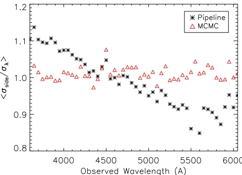
Figure 1.Wavelength dispersions,σdisp, for 236 BOSS quasar spectra randomly selected from thez =2.3, 6<S/N<8 PDF bin. The ordinate axis on the right shows the equivalent spectral resolution,R≡λ/Δλ. The dashed red lines are objects that have been discarded from the analysis because they are outliers in spectral dispersion.
same MF-PCA continuum estimation used in Lee et al. (2013),
albeit with minor modifications as described in Section 3.2.
We select only quasars that appear to be well described by the continuum basis templates, based on the goodness-of-fit to the quasar spectrum redward of Lyα. This is flagged by the variable
CONT_FLAG=1 as listed in the Lee et al. (2013) catalog (see Table 3 in that paper). Broad absorption line (BAL) quasars, the continua of which are difficult to estimate due to broad intrinsic absorption troughs, have already been discarded from the Lee et al. (2013) sample.
Another consideration is that the shape of the transmission PDF is affected by the resolution of the spectrum, especially
since the BOSS spectrographs do not resolve the Lyαforest.
The exact spectral resolution of a BOSS spectrum at a given wavelength varies as a function of both observing conditions and row position on the BOSS CCDs. The BOSS pipeline reports the wavelength dispersion at each pixel,σdisp, in units of the
co-added wavelength pixel size (binned such that ln(10)Δ(λ)/λ=
10−4). This is related to the resolving power byR ≈(2.35×
1 × 10−4ln 10σ
disp)−1. Palanque-Delabrouille et al. (2013)
have recently found, using their own analysis of the width of the arc-lamp lines and bright sky emission lines, that the spectral dispersion reported by the pipeline had a bias that depended on the CCD row and increased with wavelength,
up to 10% at λ ≈ 6000 Å. We will correct for this bias
when creating mock spectra to compare with the data, as described in Section4. Figure1shows the (uncorrected) pixel
dispersions from 236 BOSS quasars from the z = 2.3,
S/N = 6–8 bin, as a function of wavelength at the blue end
(λ=3700–4200 Å) of the spectrograph. At a fixed wavelength, there are outliers that contribute to the large spread inσdisp, e.g.,
ranging fromσdisp ≈0.9–1.8 at 3700 Å. We therefore discard
spectra with outlying values of σdisp based on the following
criterion: we first rank-order the spectra based on their σdisp
value evaluated at the central wavelength of each PDF bin (i.e.,
λ = [4012,4377,4863] Å atz = [2.3,2.6,3.0]), and then discard spectra below the 5th percentile and above the 90th percentile. This is illustrated by the dashed red lines in Figure1. Finally, since our noise estimation procedure uses the indi-vidual BOSS exposures, we discard objects that have less than three individual exposures available.
Figure 2.Pixel distribution of Lyαabsorber redshifts in the BOSS Lyαforest sample used in this paper, shown in bin sizes ofΔz=0.05. The different colors and line-styles denote the three redshift bins used in this paper. We have chosen these redshift bins—with the gap at 2.75< z <2.85—to match the simulation redshifts (Section4.1).
Table 1
Binning of BOSS LyαForest Transmission PDFs
LyαForest S/Na Nspecb Npixc Δvd Δze ΔXf
Redshift (pixel−1) ( km s−1)
2.15< z <2.45 6–8 1109 288442 1.99×10⁷ 219 704 8–10 501 129141 8.90×10⁶ 97.9 315
>10 561 146478 1.01×10⁷ 111 357
2.45< z <2.75 6–8 1004 229898 1.59×10⁷ 191 646 8–10 490 107001 7.38×10⁶ 88.6 300
>10 604 140843 9.71×10⁶ 117 396
2.85< z <3.15 6–8 511 108443 7.48×10⁶ 99.7 358
8–10 326 72448 5.00×10⁶ 66.7 239
>10 341 74284 5.12×10⁶ 68.3 245
Notes.
aMedian S/N within Lyαforest. bNumber of contributing spectra. cNumber ofΔv=69 km s−1pixels. dVelocity path length.
eRedshift path length.
fAbsorption distance, wheredX/dz=(1 +z)2(ΩM(1 +z)3+Ω
Λ)−1/2. For this conversion, we assumeΩM=0.3 andΩΛ=0.7.
Our final data set comprises 3373 unique quasars with redshifts ranging from zqso = 2.255 to zqso = 3.811, and a
median S/N of S/N = 8.08 pixel−1. This data set represents
only a small subsample of the BOSS DR9 quasar spectra, but is over two orders of magnitude larger than high-resolution quasar samples previously used for transmission PDF analysis. Table1 summarizes our data sample, and the statistics of the redshifts
and S/N bins for which we measure the transmission PDF.
Figure2shows histograms of the pixels used in our analysis, as a function of absorption redshift.
3. MEASURING THE TRANSMISSION PDF FROM BOSS
In this section, we will measure the Lyα forest
transmis-sion PDF from BOSS. In principle, the transmistransmis-sion PDF is
simply the histogram of the transmitted flux in the Lyα
[image:4.612.45.289.54.228.2]probabilistic method for co-adding the individual BOSS expo-sures that will enable us to have an accurate noise estimate. We will also describe the continuum-estimation method with which we normalize the forest transmission.
3.1. Co-addition of Multiple Exposures and Noise Estimation
Since we intend to model BOSS spectra with modest S/N,
we need an accurate estimate of the pixel noise that also allows us to separate out the contributions from Poisson noise due to the background and sky as well as read noise from the detector. In this subsection, we will construct an accurate probabilistic model of the flux and noise of the BOSS spectrograph, based on the individual exposure data that BOSS delivers.
The basic BOSS spectral data consists of a spectrum of each raw exposure,fλi(inclusive of noise), an estimate of the skysλi,
and a calibration vectorSλi, whereiindicates the exposure of the
nexpexposures taken.19The quantitys
λiis the actual sky model
that was subtracted from the fiber spectra in the extraction. The calibration vector is defined asSλi ≡fλi/fN i, withfN i being
the flux of exposureiin units of photoelectrons. The idlspec2d pipeline then estimates the co-added spectrum of the true object flux,Fλ, from the raw individual exposures, sky estimates, and
calibration vectors.
The BOSS data reduction pipeline also delivers noise es-timates in the form of variance vectors, which are, however,
known to be inaccurate (McDonald et al. 2006; Desjacques
et al.2007; Lee et al.2013; Palanque-Delabrouille et al.2013). To quantify the fidelity of the BOSS noise estimate, we used the so-called “side-band” method described in Lee et al.
(2014b) and Palanque-Delabrouille et al. (2013), which uses
the variance in flat, absorption-free regions of the quasar spectra to quantify the fidelity of the noise estimate. First, we randomly selected 10,000 BOSS quasars (omitting BAL quasars) from the Pˆaris et al. (2012) catalog in the redshift range 1.4zqso<3.4, evenly distributed into 20 redshift bins of width Δzqso = 0.1 (i.e., 500 objects per bin). We then consider the flat 1460 Å< λrest<1510 Å spectral region in the quasar
rest-frame, which is dominated by the smooth power-law continuum and relatively unaffected by broad emission lines (e.g., Vanden Berk et al.2001; Suzuki2006) or absorption lines. The pixel variance in this flat portion of the spectrum should therefore be dominated by spectral noise, allowing us to examine whether the noise estimate provided by the pipeline is accurate. We then evaluate the ratio ofσside, the pixel flux rms in the rest-frame
1460 Å< λrest<1510 Å region divided by the average pipeline
noise estimate,σλ:
σside σλ
=
fλ2− ¯fλ21/2
σλ
, (3)
where the summations and average flux is evaluated in the quasar rest-frame 1460 Å< λrest<1510 Å.
In Figure3, this quantity is averaged over the 500 individual quasars per redshift bin and plotted as a function of the observed
wavelength corresponding to λ = (1 +zqso)1485 Å. With
a perfect noise estimate, σside/σλ should be unity at all
wavelengths, but we see that the BOSS pipeline underestimates
the true noise in the spectra atλ5000 Å, by up to∼15% at
[image:5.612.321.565.53.230.2]19 Typically there arenexp=5 exposures of 15 minutes each, although this can vary due to the requirements to achieve a given (S/N)2over each individual plug-plate, as determined by the overall BOSS survey strategy (see Dawson et al.2013).
Figure 3.Quantitative test of the noise estimation fidelity in the spectra. Each point shows the ratio of the pixel variance divided by the estimated noise variance, averaged over the rest-frame 1460 Å< λrest<1510 Å flat spectral region of 500 BOSS quasars within redshift bins ofΔzqso =0.1 and plotted as a function of the corresponding observed wavelength of the flat spectral region. If there is no bias in the noise estimation, this ratio should be unity. The black asterisks show this quantity estimated using the BOSS pipeline co-added spectra and noise estimates, while the red triangles show the results from the Markov Chain Monte Carlo (MCMC) co-addition and noise estimation procedure described in Section3.1. The MCMC method clearly provides a better noise estimation than the BOSS pipeline.
the blue end of the spectra, with an overall tilt that changes
over to an overestimate atλ 4500 Å. Lee et al. (2013) and
Palanque-Delabrouille et al. (2013) provide a set of correction vectors that can be applied to the pipeline noise estimates to bring the latter to within several percent of the true noise level across the wavelength coverage of the blue spectrograph.
Unfortunately, these noise corrections are inadequate for our purposes, since we want to generate realistic mock spectra that have different realizations of the Lyαforest transmission field from the actual spectra, i.e., a differentFλ. We therefore require
a method that not only accurately estimates the noise in a given BOSS spectrum, but also separates out the photon-counting and CCD terms in the variance that results from applying the Horne (1986) optimal spectral extraction algorithm:
σλ2=Sλ(Fλ+sλ) +Sλ2σRN2 , (4)
whereσRNis the CCD read-noise.
To resolve this issue, we apply our own novel statistical method to the individual BOSS exposures to generate co-added spectra while simultaneously estimating the correspond-ing noise parameters for each individual spectrum. This proce-dure, which uses a Gibbs-sampled Markov-Chain Monte Carlo
(MCMC) algorithm, is described in detail in the Appendix.
Initially, we attempted to model the noise with just a single constant noise parameter that rescales the read-noise term of Equation (4), but this was found to be inadequate. This is likely because an optimal extraction algorithm weights by the product of the S/N and object profile, causing the corresponding vari-ance to have a non-linear dependence on the flux and sky level. Furthermore, systematic errors in the reduction, sky-subtraction and calibration will result in additional noise contributions, which could depend on sky level, object flux, or wavelength, hence deviating from this simple model.
After considerable trial-and-error to find a model that
directly from the BOSS pipeline.
In addition, we assume that the pixel noise can be modeled as a Gaussian distribution with a variance given by Equation (5). The first, photon counting, term in the equation should formally be modeled as a Poisson distribution, but since the BOSS
spectrograph always receives30–40 counts even at the blue
end of the spectrograph where the counts are the lowest, it is reasonable to use the Gaussian approximation because even in the limit of low S/N (i.e., when the spectrum is dominated by the sky flux), the moderate resolution ensures that there are at least several dozen sky photons per pixel in each exposure.
For each BOSS spectrum, we use the MCMC procedure
described in theAppendixto combine the multiple exposures
while simultaneously estimating the noise parametersAj and
true observed spectrum,Fλ. With the optimal estimates ofAj
andFλ for a given spectrum, the estimated noise variance is
then simply Equation (5).
An important advantage of the form in Equation (5) is that the object photon noise∝ Fλis explicitly separated out. This
facilitates the construction of a mock spectrum with the same noise characteristics as a true spectrum, but with a different spectral flux. For example, a mock spectrum of the Lyαforest will have a very different transmission field than the original data, and so the variance due to object photon counting noise can be added appropriately, in addition to contributions from
the known sky, and the read noise term (Equation (5)). Our
empirical determination of the parameters governing this noise model for each individual spectrum form a crucial ingredient in our forward model, which we will describe in Section4.
Our MCMC procedure works for spectra from a single camera, either red or blue; we have not yet generalized it to combine blue and red spectra of each object. However, the spectral range of the blue camera alone (≈3600–6400 Å) covers the Lyα forest up to z∼5, i.e., most practical redshifts for Lyαforest analysis. For the purposes of this paper, we restrict ourselves to spectra from the blue camera alone.
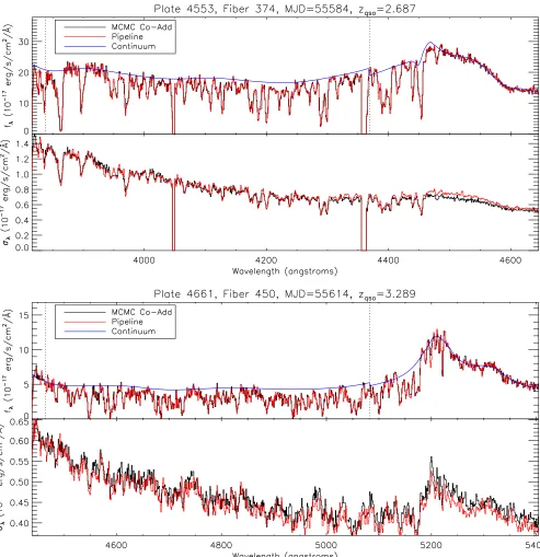
In Figures4 and5, we show examples of co-added BOSS
quasar spectra, using both the MCMC procedure and the stan-dard BOSS pipeline. In the upper panels, the MCMC co-adds are not noticeably different from the BOSS pipeline, although the numerical values are different. In the lower panels, we show the estimated noise from both methods—the differences are larger than in the fluxes but still difficult to distinguish by eye.
We therefore return to the statistical analysis by calculating
σside/σλ, the ratio of the pixel variance against the estimated
noise from the flat 1460 Å< λrest<1510 Å region of BOSS
quasars; this ratio, computed for our MCMC coadds, is plotted in Figure3. With these new co-adds, we see that this ratio is
this, therefore we regard our noise estimates as adequate for the subsequent transmission PDF analysis, without requiring any further correction.
3.2. Mean-Flux Regulated Continuum Estimation
In order to obtain the transmitted fluxFof the Lyαforest20we first need to divide the observed flux,Fλ, by an estimate for the
quasar continuum,c. We use the version of MF-PCA continuum
fitting (Lee et al.2012) described in Lee et al. (2013). Initially, PCA fitting with eight eigenvectors is performed on each quasar
spectrum redward of the Lyα line (λrest = 1216–1600 Å) in
order to obtain a prediction for the continuum shape in the
λrest<1216 Å Lyα forest region (e.g., Suzuki et al. 2005).
The slope and amplitude of this initial continuum estimate is then corrected to agree with the Lyαforest mean transmission,
Fcont(z), at the corresponding absorber redshifts, using a linear correction function.
The only difference in our continuum-fitting with that in
Lee et al. (2013) is that here we use the latest mean flux
measurements of Becker et al. (2013) to constrain our continua. Their final result yielded the power-law redshift evolution of the effective optical depth in the unshielded Lyα forest, defined
in their paper as NHi 1017.2 cm−2 (although they only
removed contributions fromNHi1019cm−2absorbers). This
is given by
τLyα,B13(z)≡ −ln(F(z))=τ0
1 +z
1 +z0
β
+C, (7)
with best-fit values of [τ0, β, C] = [0.751,2.90,−0.132] at z0=3.5.
However, the actual raw measurement made by Becker et al. (2013) is the effective total absorption within the Lyα forest region of their quasars, which also contain contributions from metals and optically thick systems:
τeff(z)≡τLyα,B13(z) +τmetals+τLLS(z), (8)
whereτmetalsandτLLS(z) denote the IGM optical depth contri-butions from metals and LLSs, respectively. For the purposes of our continuum-fitting, the quantity we require isτeff(z), since the τmetals and τLLS(z) contributions are also present in our
BOSS spectra. Becker et al. (2013) did not publish their raw
τeff(z), therefore we must now “uncorrect” the metal and LLS
Figure 4.Examples of co-added BOSS spectra from the MCMC procedure described in Section3.1(red) and from the BOSS pipeline (black) are shown in the upper panels, in the rest-frame interval 1035–1260 Å. The corresponding pixel noise estimates are shown in the upper panels. The blue line shows the MF-PCA continuum used to extract the Lyαforest transmitted flux, while the vertical dotted lines delineate the 1041–1185 Å rest-frame interval, which we define as the Lyαforest. The continuum discontinuity atλrest=1185 Å is where we have applied the “mean flux regulation” correction to the Lyαforest. In the top figure, masked pixels have had their flux and noise set to zero. The signal-to-noise ratios for the two spectra are S/N≈11 (top) and S/N≈6 (bottom) within the Lyαforest.
contributions from the publishedτLyα,B13(z). The discussion
be-low therefore attempts to retrace their footsteps and does not necessarily reflect our own beliefs regarding the actual level of these contributions.
We find τmetals = 0.02525 by simply averaging over the
Schaye et al. (2003) metal correction tabulated by
Faucher-Gigu`ere et al. (2008) (i.e., the 2.2z2.5 values inΔz=0.1 bins from their Table 4), that were used by Becker et al. (2013) to normalize their relative mean flux measurements. Note that there is no redshift dependence onτmetalsin this context, because
Becker et al. (2013) argued that the metal contribution does not
vary significantly over their redshift range. Whether or not this is really true is unimportant to us at the moment, since we are merely “uncorrecting” their measurement.
The LLS contribution to the optical depth is re-introduced by integrating over f(NHi, b, z), the column-density distribution
of neutral hydrogen absorbers:
τLLS(z)≈
1 +z λLyα
Nmax
Nmin
dNHi
db
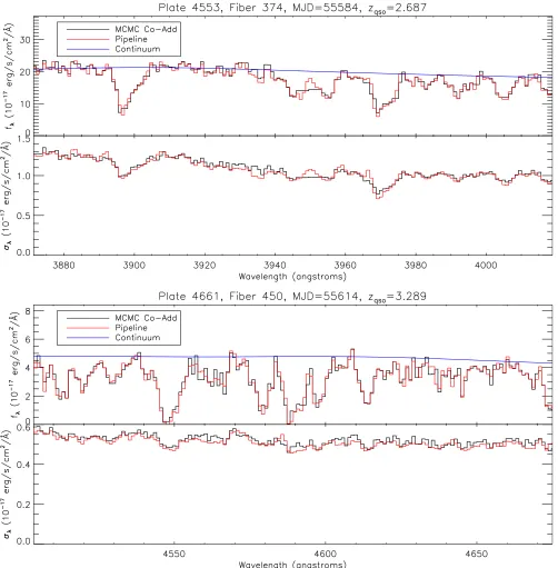
Figure 5.Same as Figure4, but the 1050 Å< λrest<1090 Å rest-frame region is expanded to better illustrate the differences between the MCMC and pipeline co-added spectra.
whereb is the Doppler parameter andW0(NHi, b) is the
rest-frame equivalent width (EW; we use the analytic approximation given by Draine2011, valid in the saturated regime).
Following Becker et al. (2013), we adopted a fixed value of
b = 20 km s−1 and assumed thatf(NHi, z) = f(NHi)dn/dz,
where f(NHi) is given by the z = 3.7 broken power-law
column density distribution of Prochaska et al. (2010) and
dn/dz∝(1 +z)2. Becker et al. (2013) had corrected for
super-LLSs and DLAs in the column-density range [Nmin, Nmax] =
[1019cm−2,1022cm−2], but as discussed above we have dis-carded all sightlines that include NHi 1020.3cm−2 DLAs;
therefore, we reintroduce the optical depth contribution for super-LLSs, i.e., [Nmin, Nmax]=[1019cm−2,1020.3cm−2]. We
findτLLS(z)=0.0022×[(1 +z)/3]3. This is a small correction,
giving rise to only a 0.5% change inFatz=3.0.
This estimate of the raw absorption, Feff(z) =
exp[−τeff(z)], is now the constraint used to fit the continua of
the BOSS quasars, i.e., we set Fcont = Feff(z). Note that
in our subsequent modeling of the data, we will use the same
Fcont(z) to fit the mock spectra to ensure an equal treatment
be-tween data and mocks. SinceFcont(z) includes a contribution fromNHi<1020.3cm−2optically thick systems, our mock
spec-tra will need to account for these systems as we shall describe in Section4.2.
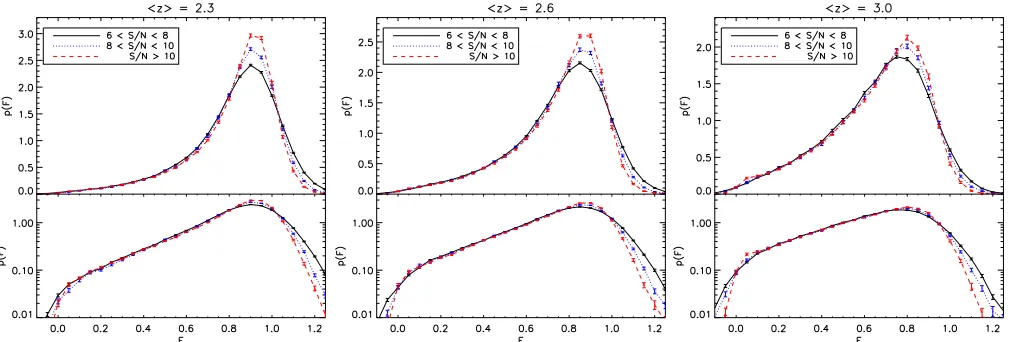
Figure 6.Lyαforest transmission PDFs,p(F), measured from different subsamples of our BOSS sample, at various redshift (withΔz=0.3) and S/N. Both the upper and lower panels show the PDF, but with linear and logarithmic ordinate axes, respectively. The different colors and line styles denote our different S/N subsamples at each redshift. The error bars are estimated from bootstrap resampling overΔv=2×10⁴km s−1segments from the contributing spectra. Table1summarizes the number of spectra and pixels that contribute to each bin.
in the previous section, we work with co-added BOSS spectra from only the blue cameras coveringλ6400 Å; this covers the full 1000–1600 Å interval required for the PCA fitting only for
z3 quasars. However, the differences in the fluxes between our MCMC co-adds and the BOSS pipeline co-adds are relatively small, and we do not expect the relative shape of the quasar spectrum to vary significantly. We can thus carry out PCA fitting on the BOSS pipeline co-adds, which cover the full observed range (3700–10000 Å), to predict the overall quasar continuum shape. This initial prediction is then used to perform mean flux regulation using the MCMC co-adds and noise estimates, to fine-tune the amplitude of the continuum fits.
The observed flux,fλ, is divided by the continuum estimate,
c, to derive the Lyαforest transmission, F = fλ/c. For each
quasar, we define the Lyαforest as the rest wavelength interval 1041–1185 Å. This wavelength range conservatively avoids the quasar’s Lyβ/Ovi emission line blend by Δv∼3000 km s−1
on the blue end, as well as the proximity zone close to the quasar redshift by stayingΔv∼10,000 km s−1from the nominal quasar systemic redshift. We are now in a position to measure the transmission PDF, which is simply the histogram of pixel transmissionsF ≡exp(−τ).
3.3. Observed Transmission PDF from BOSS
Since the Lyαforest evolves as a function of redshift, we
measure the BOSS Lyαforest transmission PDF in three bins
with mean redshifts ofz = 2.3,z = 2.6, andz =3.0, and bin sizes ofΔz=0.3. These redshift bins were chosen to match the simulations outputs (Section4.1) that we will later use to make mock spectra to compare with the observed PDF; this choice of binning leads to the gap at 2.75< z <2.85 as seen in Figure2. In this paper, we restrict ourselves toz3 since the primary purpose is to develop the machinery to model the BOSS spectra. In subsequent papers, we will apply these techniques to
analyze the transmission PDF in the full 2z4 range using
the larger samples of subsequent BOSS data releases (DR10; Ahn et al.2014).
Another consideration is that the transmission PDF is strongly affected by the noise in the data. While we will model this effect in detail (Section 4), there is a large distribution of S/N within our subsample ranging from S/N = 6 pixel−1 to
S/N∼20 pixel−1. We therefore further divide the sample into
three bins depending on the median S/N per pixel within the Lyα
forest: 6<S/N<8, 8<S/N<10, S/N>10. The consistency of our results across the S/N bins will act as an important check for the robustness of our noise model (Section3.1).
We now have nine redshift and S/N bins in which we
evaluate the transmission PDF from BOSS; the sample sizes
are summarized in Table 1. For each bin, we have selected
quasars that have at least 30 Lyαforest pixels within the required redshift range, and which occupy the quasar rest-frame interval 1041–1185 Å. The co-added spectrum is divided with its MF-PCA continuum estimate (described in the previous section) to obtain the transmitted flux, F, in the desired pixels. We then compute the transmission PDF from these pixels.
Physically, the possible values of the Lyαforest transmission
range fromF =0 (full absorption) toF =1 (no absorption).
However, the noise in the BOSS Lyα forest pixels, as well
as continuum fitting errors, leads to pixels with F <0 and
F > 1. We therefore measure the transmission PDF in the range −0.2< F <1.5, in 35 bins with width Δ(F) = 0.05, and normalized such that the area under the curve is unity. The statistical errors on the transmission PDF are estimated by
the following method: we concatenate all the individual Lyα
forest segments that contribute to each PDF, and then carry out bootstrap resampling overΔv=2×10⁴km s−1segments with
200 iterations. This choice ofΔv corresponds to∼250–300 Å
in the observed frame atz∼2–3—according to Rollinde et al.
(2013), this choice ofΔv and number of iterations should be sufficient for the errors to converge (see also Appendix B in McDonald et al.2000).
In Figure 6, we show the Lyα forest transmission PDF
measured from the various redshift and S/N subsamples in our
BOSS sample. At fixed redshift, the PDFs from the lower S/N
data have a broader shape as expected from increased noise variance. With increasing redshift, there are more absorbed
pixels, causing the transmission PDFs to shift toward lowerF
values. As discussed previously, there is a significant portion of F >1 pixels due to a combination of pixel noise and continuum errors, with a greater proportion of F >1 pixels
in the lower-S/N subsamples as expected. Unlike the
high-resolution transmission PDF, at z3 there are few pixels
Figure 7.Top: 2D density plot of the error covariance matrix for the Lyα forest transmission PDF from thez =2.6, S/N=8–10 BOSS subsample as a function of transmission bins, along with (bottom) the corresponding correlation function. The covariance matrix was estimated through bootstrap resampling, and the values have been multiplied by 104 for clarity. The covariances are largely diagonal, except for some cross-correlations between neighboring bins.
the BOSS spectrograph, which smooths over the observed
Lyα forest such that even saturated Lyα forest absorbers
withNHi1014–1016cm−2rarely reach transmission values of
F0.3. The pixels withF0.3 are usually contributed either by blends of absorbers or optically thick LLSs (see also Pieri et al.2014).
An advantage of our large sample size is that it is also able to directly estimate the error covariances,Cboot, via bootstrap
resampling—an example is shown in Figure7. In contrast to
the Lyα forest transmission PDF from high-resolution data
which have significant off-diagonal covariances (Bolton et al.
2008), the error covariance from the BOSS transmission PDF
is nearly diagonal with just some small correlations between neighboring bins, although we also see some anti-correlation between transmission bins atF∼0.8 andF∼1.
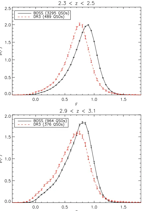
It is interesting to compare the transmission PDF from our
data with that measured by Desjacques et al. (2007) from
[image:10.612.47.295.56.470.2]SDSS DR3. This comparison is shown in Figure8, in which
Figure 8.Comparison between the Lyαforest transmission PDFs measured from our BOSS DR9 sample (solid black lines), and the SDSS DR3 sample from Desjacques et al. (2007; dashed red lines). Only sightlines with S/N>4 were used in evaluating these PDFs. The lower average transmission of the DR3 PDFs is because Desjacques et al. (2007) had directly extrapolated a power law fromλrest > 1216 Å for continuum estimates, which does not take into account a flattening of the quasar continuum that occurs atλrest∼1200 Å; our BOSS spectra, in contrast, have been normalized to mean transmission values in agreement with the latest measurements and takes this effect into account.
the transmission PDFs calculated from SDSS DR3 Lyαforest
spectra with S/N >4 (kindly provided by Dr. V. Desjacques) are shown for two redshift bins, juxtaposed with the BOSS transmission PDFs calculated from spectra with the same redshift and S/N cuts.
While there is some resemblance between the two PDFs, the most immediate difference is that the Desjacques et al. (2007) PDFs are shifted to lower transmission values, i.e., the mean transmission,F, is considerably smaller than that from our BOSS data: F(z = 2.4) = 0.73 and F(z = 3.0) =
0.64 from their measurement, whereas the BOSS PDFs have
F(z=2.4)=0.80 andF(z=3.0)=0.70. This difference arises because the Desjacques et al. (2007) used a power-law continuum (albeit with corrections for the weak emission lines in the quasar continuum) extrapolated fromλrest >1216 Å in
the quasar rest-frame; this does not take into account the power-law break that appears to occur in low-redshift quasar spectra atλrest ≈ 1200 Å (Telfer et al.2002; Suzuki2006). Later in
measurements. Our continua, in contrast, have been constrained
to match existing measurements of F(z), for which there
is good agreement between different authors at z3 (e.g.,
Faucher-Gigu`ere et al.2008; Becker et al.2013).
Another point of interest in Figure8is that the error bars of the BOSS sample are considerably smaller than those of the earlier measurement. This difference is largely due to the significantly larger sample size of BOSS. The proportion of pixels withF0 appears to be smaller in the BOSS PDFs compared with the older data set, but this is because Desjacques et al. (2007) did not remove DLAs from their data.
We next describe the creation of mock Lyαabsorption spectra designed to match the properties of the BOSS data.
4. MODELING OF THE BOSS TRANSMISSION PDF
In this section, we will describe simulated Lyαforest mock spectra designed, through a “forward-modeling” process, to have the same characteristics as the BOSS spectra, for com-parison with the observed transmission PDFs described in the previous section. For each BOSS spectrum that contributed to our transmission PDFs in the previous section, we will take the
Lyα absorption from randomly selected simulation sightlines,
then introduce the characteristics of the observed spectrum using auxiliary information returned by our pipeline.
Starting with simulated spectra from a set of detailed hydro-dynamical IGM simulations, we carry out the following steps, which we will describe in turn in the subsequent subsections:
1. Introduce LLS absorbers.
2. Smooth the spectrum to BOSS resolution.
3. Add metal absorption via an empirical method using
lower-redshift SDSS/BOSS quasars.
4. Add pixel noise, based on the noise properties of the real BOSS spectrum using parameters estimated by our MCMC noise estimation technique.
5. Simulate continuum errors by refitting the noisy mock spectrum.
In the subsequent subsections, we will describe each step in detail. The effect of each step on the observed transmission PDF is illustrated in Figure9.
4.1. Hydrodynamical Simulations
As the basis for our mock spectra, we use hydrodynamic simulations run with a modification of the publicly available GADGET-2 code. This code implements a simplified star formation criterion (Springel et al.2005) that converts all gas particles that have an overdensity above 1000 and a temperature
below 105 K into star particles (see Viel et al. 2004). The
simulations used are described in detail in Becker et al. (2011) and in Viel et al. (2013a).
The reference model that we use is a box of length 20h−1
comoving Mpc with 2 ×5123 gas and cold DM particles
(with a gravitational softening length of 1.3h−1kpc) in a flat
ΛCDM universe with cosmological parametersΩm = 0.274,
Ωb = 0.0457, ns = 0.968, H0 = 70.2 km s−1Mpc−1 and
σ8=0.816, in agreement both with nine-yearWMAP(Komatsu
et al.2011) andPlanckdata (Planck Collaboration et al.2014). The initial condition power spectra are generated with CAMB (Lewis et al.2000). For the boxes considered in this work, we have verified that the transmission PDF has converged in terms of box size and resolution.
We explore the impact of different thermal histories on
[image:11.612.341.552.52.548.2]the Lyαforest by modifying the ultraviolet (UV) background
Figure 9. Cumulative effect of various aspects of our forward model that attempts to reproduce the Lyαforest transmission PDF from BOSS. Starting with the “raw” transmission PDF from the simulations (top), the black curve in each panel shows the PDF from the prior panel, while the red curve shows the effect from (a) the addition of LLS, (b) smoothing from the finite spectrograph resolution, (c) contamination from lower-redshift metals, (d) pixel noise, and (e) continuum fitting errors. The transmission PDF modeled in this figure is from thez =2.3, 8<S/N<10 bin.
photo-heating rates in the simulations as done in, e.g., Bolton et al. (2008). A power-law temperature–density relation,T = T0Δγ−1, arises in the low-density IGM (Δ < 10) as a natu-ral consequence of the interplay between photo-heating and adiabatic cooling (Hui et al.1997; Gnedin & Hui1998). The
value ofγ within a simulation can be modified by varying a
density-dependent heating term (see, e.g., Bolton et al.2008). We consider a range of values for the temperature at mean den-sity, T0, and the power-law index of the temperature–density
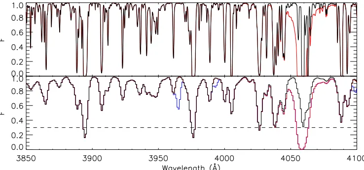
Figure 10.Simulatedz =2.3 Lyαforest skewer from our hydrodynamical simulations, without smoothing (top panel) and smoothed to BOSS resolution (bottom panel). The black curve is the simulated transmission directly extracted from the simulations, while the red curve is the same transmission field but with an LLS added atλ=4057 Å orz=2.337. The blue curve in the bottom panel shows the effect of the metal absorbers added using our empirical method. For illustrative purposes, we have specifically chosen to this simulated sightline to have significant LLS and metal absorption; it is possible for a sightline to have neither. The dashed horizontal line denotesF=0.3, below which our fiducial transmission PDF model disagrees with BOSS (see Section5).
Table 2
Evolution ofT0in Hydrodynamical Simulations
z T_COLD T_REF T_HOT
2.3 13000 K 18000 K 23000 K
2.6 11000 K 16000 K 21500 K
3.0 9000 K 14000 K 19000 K
recently by Becker et al. (2011). These consist of a set of
three different indices for the temperature–density relation,
γ(z=2.5)∼1.0,1.3,1.6, that are kept roughly constant over the redshift rangez=[2–6] and three different temperatures at mean density,T0(z = 2.5)∼[11000,16000,21500] K, which evolve with redshift, yielding a total of nine different thermal
histories. Between z = 2 andz = 3 there is some
tempera-ture evolution and the IGM becomes hotter at low redshift; at
z = 2.3, the models have T0∼[13000,18000,23000] K. We
refer to the intermediate temperature model as our “reference”
model, orT_REF, while the hot and cold models are referred
to asT_HOTandT_COLD, respectively. The values ofT0 of our
simulations at the various redshifts are summarized in Table2. Approximately 4000 core hours were required for each
simulation run to reachz= 2. The physical properties of the
Lyαforest obtained from theTree PM/SPHcodeGADGET-2
are in agreement at the percent level with those inferred from
the moving-mesh codeAREPO(Bird et al.2013) and with the
Eulerian codeENZO(O’Shea et al.2004).
For this study, the simulation outputs were saved at z =
[2.3,2.6,3.0], from which we extract 5000 optical depth sight-lines binned to 2048 pixels each. To convert these to trans-mission spectra, the optical depths were rescaled such that the skewers collectively yielded a desired mean transmission,
FLyα ≡exp(−τLyα). For our fiducial models, we would like
to use the mean transmission values estimated by Becker et al. (2013), which we denote asFLyα,B13 ≡exp(−τLyα,B13).
How-ever, their estimates assume certain corrections from optically thick systems and metal absorption. We therefore add back in the corrections they made (see discussion in Section3.2) to get their “raw” measurement forFthat now includes all optically thick systems and metals, and then remove these contributions
assum-ingourown LLS and metal absorption models (see below).
Later in the paper, we will argue that our PDF analysis in fact places independent constraints onFLyα.
4.2. Lyman-limit Systems
In principle, all optically thick Lyαabsorbers such as LLSs
and DLAs should be discarded from Lyα forest analyses,
since they do not trace the underlying matter density field in the same way as the optically thin forest (Equation (1)), and require radiative transfer simulations to accurately capture their properties (e.g., McQuinn et al.2011; Rahmati et al.2013).
While DLAs are straightforward to identify through their saturated absorption and broad damping wings even in noisy
BOSS data (see, e.g., Noterdaeme et al. 2012), the detection
completeness of optically thick systems through their Lyα ab-sorption drops rapidly atNHi1020 cm−2. Even in high-S/N,
high-resolution spectra, optically thick systems can only be reli-ably detected through their Lyαabsorption atNHi1019cm−2
(“super-LLS”). Below these column densities, optically thick systems can be identified either through their rest-frame 912 Å Lyman-limit (albeit only one per spectrum) or using higher-order Lyman-series lines (e.g., Rudie et al. 2013). Neither of these approaches have been applied in previous Lyαforest trans-mission PDF analyses (McDonald et al.2000; Kim et al.2007; Calura et al.2012; Rollinde et al.2013), so arguably all these analyses are contaminated by LLSs.
Instead of attempting to remove LLSs from our observed spectra, we incorporate them into our mock spectra through the following procedure. For each PDF bin, we evaluate the total redshift pathlength of the contributing BOSS spectra (and
corresponding mocks)—this quantity is summarized in Table1.
This is multiplied bylLLS(z), the number of LLS per unit redshift,
to give the total number of LLS expected within our sample. We used the published estimates of this quantity by Ribaudo et al. (2011)21which is valid over 0.24< z <4.9:
lLLS(z)=lz0(1 +z)γLLS, (10)
wherelz0=0.1157 andγLLS=1.83.
21 Note that the valuel
[image:12.612.72.267.312.365.2]After estimating the total number of LLSs in our mock spectra,lLLS(z)Δz, we add them at random points within our set of simulated optical depth skewers. We also experimented with adding LLSs such that they are correlated with regions that already have high column density (e.g., Font-Ribera & Miralda-Escud´e 2012), but we found little significant changes to the transmission PDF and therefore stick to the less computationally intensive random LLSs.
For each model LLS, we then draw a column density using the published LLS column density distribution,f(NHi), from
Prochaska et al. (2010). This distribution is measured atz≈3.7,
so we make the assumption that f(NHi) does not evolve
with redshift between 2z3.7. For our column densities
of interest, this distribution is represented by the broken power laws:
f(NHi)=
k1NH−0i.8 if 1017.5< N
Hi<1019.0
k2NH−1i.2 if 1019.0< N
Hi<1020.3
. (11)
For the normalizationsk1andk2, we demand that
1019.0
1017.5
k1NH−0i.8dNHi+ 1020.3
1019.0
k2NH−1i.2dNHi=1, (12)
and require both power laws to be continuous at NHi =
1019.0 cm−2. These constraints produce k
1 = 10−4.505 and k2 = 103.095. After drawing a random value for the column
density of each LLS, we add the corresponding Voigt profile to the optical depth in the simulated skewer.
In addition to the LLS with column densities of 1017.5cm−2< N
Hi<1020.3cm−2that are defined to haveτHi
2, there is also a population of partial Lyman-limit systems (pLLSs) that are not well-captured in our hydrodynamical sim-ulations since they have column densities (1016.5cm−2NHi<
1017.5cm−2) at which radiative transfer effects become
signif-icant (τHi 0.1). However, the incidence rates and
column-density distribution of pLLSs are ill-constrained since they are difficult to detect in normal LLS searches. We therefore account for the pLLS by extrapolating the low end of the power-law distribution in Equation (11) down toNHi=1016.5cm−2, i.e.,
f(1016.5cm−2< NHi<1017.5cm−2)=k1NH−i0.8. (13)
This simple extrapolation does not take into account constraints from the mean free path of ionizing photons (e.g., Prochaska
et al. 2010), which predicts a steeper slope for the pLLS
distribution, but we will explore this later in Section5.2. Comparing the integral of this extrapolated pLLS distribution with Equation (12) leads us to conclude that
lpLLS(z)=0.197lLLS(z), (14)
and we proceed to randomly add pLLSs to our mock spectra in the same way as LLSs.
The other free parameter in our LLS model is their effective
b-parameter distribution. However, due to the observational
difficulty in identifyingNHi18.5 cm−2LLSs, theb-parameter
distribution of this distribution has, to our knowledge, never been quantified. Due to this lack of knowledge, it is common to
simply adopt a singleb-value when attempting to model LLSs
(e.g., Font-Ribera & Miralda-Escud´e2012; Becker et al.2013).
We therefore assume that all our pLLSs and LLSs have ab
-parameter of b = 70 km s−1 similar to DLAs (Prochaska &
Wolfe1997), an “effective” value meant to capture the blending
of multiple Lyα components. However, the b-parameter for
this population of absorbers is a highly uncertain quantity and as we shall see, it will need to be modified to provide a satisfactory fit to the data although it will turn out to not strongly affect our conclusions regarding the IGM temperature–density relationship. Figure 10 illustrates the effect of adding a LLS to a mock spectrum, and its subsequent smoothing with the spectrograph resolution kernel (next section).
4.3. Spectral Resolution
The spectral resolution of SDSS/BOSS spectra is R ≡
λ/Δλ ≈ 1500–2500 (Smee et al. 2013). The exact value
varies significantly both as a function of wavelength, and across different fibers and plates depending on observing conditions (Figure1).
For each spectrum, the BOSS pipeline provides an estimate of the 1σ wavelength dispersion at each pixel, σdisp, in units of the co-added wavelength grid size (Δlog10λ= 10−4). The spectral resolution at that pixel can then be obtained from the dispersion, through the following conversion:R ≈(2.35×1× 10−4ln 10σ
disp)−1. Figure1shows the pixel dispersions from
236 randomly selected BOSS quasar as a function of wavelength at the blue end of the spectrograph. Even at fixed wavelength, there is a considerable spread in the dispersion, e.g., ranging from σdisp ≈ 0.9–1.8 at 3700 Å. The value of σdisp typically
decreases with wavelength (i.e., the resolution increases).
In their analysis of the Lyα forest 1D transmission power
spectrum, Palanque-Delabrouille et al. (2013) made their own study of the BOSS spectral resolution by directly analyzing the line profiles of the mercury and cadmium arc lamps used in the wavelength calibration. They found that the pipeline underestimates the spectral resolution as a function of fiber position (i.e., CCD row) and wavelength: the discrepancy is
<1% at blue wavelengths and near the CCD edges, but increases to as much as 10% atλ∼6000 Å near the center of the blue CCD (compare with Figure 4 in Palanque-Delabrouille et al.2013). Our analysis is limited toλ5045 Å, i.e.,z3.15, where the discrepancy is under 4%. Nevertheless, we implement these corrections to the BOSS resolution estimate to ensure that we model the spectral resolution to an accuracy of<1%.
For each BOSS Lyα forest segment that contributes to
the observed transmission PDFs discussed in Section 3, we
concatenate randomly selected transmission skewers from the simulations described in the previous section. This is because the simulation box size ofL=20h−1Mpc (Δv∼2000 km s−1) is significantly shorter than the path length of our redshift bins (Δz = 0.3, orΔv ≈ 27,000 km s−1). This ensures that each BOSS spectrum in our sample has a mock spectrum that is exactly matched in pathlength.
We then directly convolve the simulated skewers by a Gaus-sian kernel with a standard deviation that varies with wave-length, using the estimated resolution from the real spectrum, multiplied by the Palanque-Delabrouille et al. (2013) resolution corrections. The effect of smoothing on the transmission PDF is illustrated by the dashed red curve in Figure9(b). Smooth-ing decreases the proportion of pixels with high transmission
(F ≈1) and with high absorption (F ≈0), and increases the
number of pixels with intermediate transmission values.
4.4. Metal Contamination
Metal absorption along our observed Lyα forest sightlines
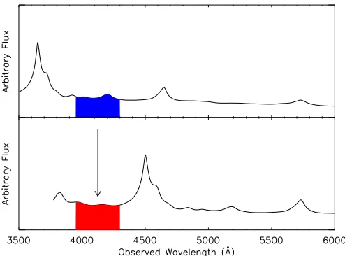
Figure 11.Illustration of our empirical “sideband” model of metal contami-nation in our mock Lyαforest spectra. The lower panel shows thezqso=2.7 quasar along with its Lyαforest region (red) that we wish to model. To its corre-sponding mock spectrum, we add metals observed in theλrest≈1260–1390 Å region of a lower-redshift (zqso=2.0) quasar (blue region in top panel).
statistics of the Lyαforest. In high-resolution data, this contam-ination is usually treated by directly identifying and masking the metal absorbers, although in the presence of line blending it is unclear how thorough this approach can be.
With the lower S/N and moderate resolution of the BOSS
data, direct metal identification and masking is not a viable approach. Furthermore, most of the weak metal absorbers seen in high-resolution spectra are not resolved in the BOSS data.
Rather than removing metals from the BOSS Lyα forest
spectra, we instead add metals as observed in lower-redshift quasar spectra. In other words, we add absorbers observed in the rest-frameλrest≈1260–1390 Å region of lower-redshift quasars
with 1+zqso≈(1216 Å/1300 Å)(1+z), such that the observed
wavelengths are matched to the Lyαforest segment with average
mock spectra, which are not well sampled by the BOSS target
selection (Ross et al.2012). We emphasize that we work with
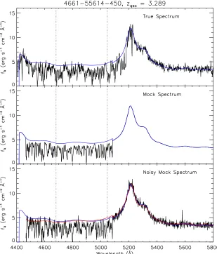
the “raw” absorber catalog, i.e., the individual absorption lines have not been identified in terms of metal species or redshift. For each quasar, the catalog provides a line list with the observed wavelength, EW (Wr), FWHM, and detection S/N,Wr/σWr. To ensure a clean catalog, we use onlyWr/σWr 3.5 absorbers in the catalog that were identified from quasar spectra with S/N >15 per angstrom redward of Lyα. The latter criterion ensures that even relatively weak lines (with EW0.5 Å) are accounted for in our catalog. Figure12shows an example of the lower-redshift quasar spectra that we use for the metal modeling. However, we want to add a smooth model of the metal-line absorption to add to our mock spectra, rather than adding in a noisy spectrum. We therefore use a simple model as follows:
For each Lyα forest segment we wish to model at redshift
z, we select an absorber line-list from a random quasar with 1 +zqso ≈(1216 Å/1300 Å)(1 +z). We next assume that all
resolved metals in the SDSS/BOSS spectra are saturated and
22 Siiiian obvious exception, although we will later account for this omission in our error bars (Section5.3).
[image:14.612.151.465.481.689.2]