Self labeling techniques for semi supervised time series classification: an empirical study

(1)

Systems

Self-labeling techniques for

semi-supervised time series

classification: an empirical study

Mabel Gonz´

alez

1

_{, Christoph Bergmeir}

2

_{, Isaac Triguero}

3

_{, Yanet Rodr´ıguez}

1

_{and Jos´}

_{e M. Ben´ıtez}

4

1_{Department of Computer Science, Universidad Central “Marta Abreu” de Las Villas, Cuba;} 2_{Faculty of Information Technology, Monash University, Melbourne, Australia;}3_{School of Computer}

Science, University of Nottingham, United Kingdom;4_{Department of Computer Science and Artificial}

Intelligence, E.T.S. de Ingenier´ıas Inform´atica y de Telecomunicaci´on, University of Granada, Spain

Abstract. An increasing amount of unlabeled time series data available renders the semi-supervised paradigm a suitable approach to tackle classification problems with a reduced quantity of labeled data. Self-labeled techniques stand out from semi-supervised classification methods due to their simplicity and the lack of strong assumptions about the distribution of the labeled and unlabeled data. This paper addresses the relevance of these techniques in the time series classification context by means of an empirical study that compares successful self-labeled methods in conjunction with various learn-ing schemes and dissimilarity measures. Our experiments involve 35 time series datasets with different ratios of labeled data, aiming to measure the transductive and inductive classification capabilities of the self-labeled methods studied. The results show that the nearest-neighbor rule is a robust choice for the base classifier. In addition, the amend-ing and multi-classifier self-labeled based approaches reveal a promisamend-ing attempt to perform semi-supervised classification in the time series context.

Keywords: supervised classification; Self-labeled; Time series classification; Semi-supervised learning; Self-training

1. Introduction

In the time series field, the semi-supervised learning (SSL, Chapelle et al., 2006) paradigm has received a lot of research attention during the past decade. As cheap sensors of all kinds become more and more available, vast amounts of

(2)

unlabeled time series data are generated. By contrast, the cost related to the labeling process makes it often unfeasible to obtain a fully labeled training set. In this situation, SSL is a good solution to improve the learning accuracy tak-ing advantage of the unlabeled data in conjunction with a small set of labeled data. Specifically, semi-supervised classification (SSC) focuses on training a clas-sifier such that it outperforms a supervised clasclas-sifier trained on the labeled data alone. In the time series domain, SSL has found a wide range of applications such as the classification of flying insects (Batista et al., 2011), web informa-tion extracinforma-tion (Flesca et al., 2007), and failure predicinforma-tion in oil producinforma-tion (Liu et al., 2011), among others. In this work, we tackle SSC problems in the time series classification context.

Time series data is characterized by a high dimensionality and its numeri-cal and continuous nature. Therefore, a special treatment must be considered to deal with time series classification (Fu, 2011). A first category of proposals, called

feature-basedapproach (Carden and Brownjohn, 2008; Behera et al., 2010; Weng

and Shen, 2008; Dash et al., 2008; Fulcher and Jones, 2014), transforms the original time series into a new description space where conventional classifiers can be applied. Signal processing or statistical tools are commonly used to ex-tract features from the original raw data. A second category (Rodr´ıguez et al., 2000; Povinelli et al., 2004; Douzal-Chouakria and Amblard, 2012; Rodr´ıguez and Alonso, 2004; Xi et al., 2006; Kaya and Gunduz-Oguducu, 2015) focuses on customizing or developing classifiers specifically designed for time series data. This category, which includes theinstance-based approach, is mostly based on the selection of an appropriate representation of the time series and a suit-able measure of dissimilarity. Several representations and dissimilarity mea-sures have been proposed to deal with the time series classification problem including: spectral approaches (Faloutsos et al., 1994), autocorrelation function (Bagnall and Janacek, 2004) and elastic measures (Sakoe and Chiba, 1978; Chen et al., 2005; Marteau, 2009), among others. Our paper considers this second approach.

Several SSC approaches have been applied to the time series classification problem. The work of Marussy and Buza (2013) uses the cluster-then-label ap-proach by a constrained hierarchical single link clustering method. The work of Frank et al. (2013) applies a similar approach with a similarity measure called geometric template matching. The applicability of graph-based methods to time series classification is addressed in various works (De Sousa et al., 2014; De Sousa et al., 2015). The classical semi-supervised support vector machines method is extended to tackle time series classification by Kim (2013).

Another family of SSC methods, denoted self-labeled techniques (Triguero et al., 2015), aims to enlarge the original labeled set using the most confident predictions to classify unlabeled data. In contrast to the previous mentioned approaches, self-labeled techniques do not make any special assumptions about the distribution of the input data. Self-training (Yarowsky, 1995) and co-training (Blum and Mitchell, 1998) are the most popular self-labeled techniques. Both approaches have been applied in a time series context.

(3)

conjunction with the self-training, thek-nearest-neighbor (kNN, Aha et al., 1991) is typically used as the base learner as it has shown to be particularly effective for time series classification tasks (Serr`a and Arcos, 2014; Wang et al., 2013).

Co-training is a SSC method that requires two conditionally independent views which are sufficient for learning and classification. For each view, the unla-beled instances with highest confidence are selected and launla-beled to be turned into additional training data for the other view. The multi-view requirement of the co-training technique is typically too strong and difficult to meet in the time series domain where in most cases observations close together are correlated. The work of Meng et al. (2011) applies a variant of co-training (Goldman and Zhou, 2000) which uses the hidden Markov model (Rabiner, 1989) and one-nearest-neighbor (1NN) as two different learners instead of the classical two views of the data.

There are various works in the literature (Begum et al., 2014; Chen et al., 2013; Ratanamahatana and Wanichsan, 2008; Wei and Keogh, 2006; Meng et al., 2011) that focus on the SSC of time series, which involve self-labeled techniques. Self-training and co-training are the only self-labeled techniques that have been applied in a time series context so far, to the best of our knowledge. Our study broadens this approach to other self-labeled techniques, therewith gaining new insights and allowing for more detailed conclusions on this topic. Moreover, de-spite the successful application of 1NN to time series classification tasks, the use of different learning approaches as a base classifiers seems to be an under-explored area. These reasons motivate our paper, which has three main objectives as follows:

– To explore the applicability of classical self-labeled techniques in the time series domain, as well as the use of other classification schemes as base learners in addition to the well-known 1NN.

– To identify the best methods for each base learner under different ratios of labeled data and dissimilarity measures.

– To determine the influence of the geometrical characteristics of time series datasets in the performance of the self-labeled techniques.

The rest of the paper is organized as follows. In Section 2, we provide defini-tions and the notation of SSC in the time series domain. Furthermore, we discuss the main characteristics of the self-labeled techniques and the base learners in-volved in this study. In Section 3, we introduce the experimental framework. In Section 4, we present the results obtained and discuss them. Finally, Section 5 concludes the paper.

2. Semi-supervised time series classification

In this section we define the SSC of time series problem and the principal notation and definitions. Furthermore, we review the self-labeled techniques and the base learner methods involved in this study (Sections 2.1 and 2.2).

In SSC, the source dataset has two parts, L and U. Let L be the set of instances{x1, . . ., xl}for which the labels{y1, . . ., yl}are provided. LetU be the

set of instances{xl+1, . . ., xl+u} for which the labels are not known. We follow

the typical assumption that there is much more unlabeled than labeled data, i.e.,

ul. The whole setL∪U forms the training set.

(4)

uni-variate, real-valued, and evenly spaced time series. In this case, the time series

xi = [p1, p2, . . . , pn] is considered a sequence of1-dimensional data points.

Depending on the goal, we can categorize SSC into two slightly different settings (Chapelle et al., 2006), namely transductive and inductive learning. The former is devoted to predict the labels on the unlabeled instancesU provided during the training phase. The latter aims to predict the labels on unseen testing instances. In this work, we delve into both settings aiming to perform an extensive analysis of the selected methods.

2.1. Self-labeled Techniques

Self-labeled techniques follow a wrapper methodology using one or more su-pervised classifiers to determine the most likely class of the unlabeled instances during an iterative process. The base classifier(s) play(s) a crucial role in the esti-mation of the most confident instances ofU. The main feature that distinguishes self-labeled methods is the way they obtain one or several enlarged labeled sets to efficiently represent the learned hypothesis from the training set. In the liter-ature, there are several proposals that follow this approach which differ mainly in the following aspects:

– Addition mechanism: There is a variety of schemes in which the enlarged

set can be formed. The most used ones areincrementalandamending. The former adds, step-by-step, the most confident instances fromU to the enlarged set. The latter allows rectifications to already labeled instances to avoid the introduction of noisy instances in the enlarged set(s).

– Classification model: Self-labeled techniques can use one or more base clas-sifiers to establish the class of unlabeled instances. Single-classifier models assign to each instance the most likely class considering the used classifier. Multi-classifiermodels combine the hypothesis learned by several classifiers to estimate the class by agreement of classifiers or combination of the proba-bilities obtained by single-classifiers.

– Learning approach: Independently of the number of base classifiers, the

number of learning methods is another important issue. Thesingle-learning approach can be linked with single and multi-classifier models. By contrast, the multi-learning approach is intrinsically related to the multi-classifier model. In a multi-learning method, the different classifiers come from different learning methods.

– Stopping criterion: This is the mechanism used to stop the self-labeling pro-cess preventing the addition of labeled instances inL with a low confidence level. Often, a prefixed number of iterations is used as stopping criterion. An-other criterion used is the occurrence of non-changes in the learned hypotheses during successive iterations of the self-training process.

Since each approach has its own benefits and drawbacks, we include in this study a representative sample of methods. The selection made is based on the results obtained in the extensive overview study of Triguero et al. (Triguero et al., 2015) and it includes the following methods:

(5)

extracted and classified from U, during an iteratively and incremental pro-cess. The stopping criterion consists in a fixed number of iterations that can be adapted to the original size of U. Following a wrapper methodology, the base classifier used by self-training is considered as another parameter of the method.

– Self-training with editing (SETRED, Li and Zhou, 2005): is a self-training variant with a different addition mechanism. SETRED introduces a data edit-ing method to filter the noise examples that has been labeled by the base classifier. For each iteration, the mislabeled examples are identified using the local information provided by the neighborhood graph (Zighed et al., 2002). – Self-training nearest-neighbor rule using cut edges (SNNRCE, Wang et al.,

2010): is a variant of SETRED that includes a first stage where the most confident examples are added toL. In the next stage, the self-training standard is applied in combination with the 1NN rule as a base classifier. The iterative process stops when the expected number of examples in the minority class is reached, according to the distribution observed in L. In the final stage, the mislabeled examples are relabeled attending to the information provided by the neighborhood graph.

– Tri-training (TriT, Zhou and Li, 2005): is a variant of co-training that trains three instead of the traditional two classifiers. These classifiers have in com-mon the same learning scheme. The diversity between the base classifiers is obtained through manipulating the original setL, for example, using Bagging (Breiman, 1996). For each iteration, the selected examples fromU are labeled and added to the training set of a specific classifier only if there is agreement between the remaining classifiers and some conditions are satisfied. The stop-ping criterion is reached when the hypothesis of the three classifiers do not suffer any modification during a complete iteration.

– Democratic co-learning (Democratic, Zhou and Goldman, 2004): is a multi-classifier and multi-learning method. The specific number of multi-classifiers and its learning scheme are established as arguments of the method. Initially, all classifiers are trained using the examples in L. For each iteration, a label for each unlabeled example is proposed via majority vote. If the classification provided by a classifier disagrees with most classifiers, in a particular example, then this example is included in the training set of the classifier. The iteratively process stops when the training sets of the classifiers do not suffer any additions during a complete iteration.

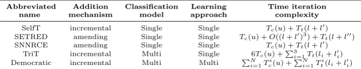
Table 1 summarizes the principal characteristics of the self-labeled methods selected.

The variety of stopping criteria, associated with the self-labeled methods makes difficult to estimate the maximum number of iterations performed by

Abbreviated Addition Classification Learning Time iteration

name mechanism model approach complexity

SelfT incremental Single Single Tc(u) +Tt(l+l0)

SETRED amending Single Single Tc(u) +O((l+l0)3) +Tt(l+l00)

SNNRCE amending Single Single Tc(u) +Tt(l+l0)

TriT incremental Multi Single 6Tc(u) +Pi3=1Tt(li+l0i)

Democratic incremental Multi Multi PN i=1T

i c(u) +

PN i=1T

[image:5.595.96.449.603.671.2]

i t(li+l0i)

(6)

each method. For simplicity, we focus the temporal analysis on the complexity related with the execution of each iteration in the main loop of the method. The algorithmic complexity is based on the current number of unlabeled examples (u) and labeled examples (l) at the beginning of the iteration. Table 1 includes the time analysis of each method. The functionsTt and Tc represent the time cost

associated with an specific learning scheme in the task of training the model and classifying new instances, respectively. l0 is the number of candidate examples selected to increase the setL and l00 is the resulting number of examples after the filtering process. In the case of the SETRED method, the construction of the neighborhood graph has a cubic complexity. For the analysis of the Democratic method we take into account the existence ofN different learning schemes.

2.2. Supervised approaches for time series classification

Different approaches have been used to face the time series classification problem such askNN classifiers, decision trees (DT) or support vector machines (SVMs). ThekNN classifier has been widely applied in the time series context (Petitjean et al., 2016; Geler et al., 2015). This classifier approximates the confidence in terms of dissimilarity between instances. There are several distance measures pre-sented in the literature that have been used for evaluating dissimilarity between time series: lock-step measures (Euclidean), feature-based measures (Fourier co-efficients), model-based measures (autocorrelation functions), and elastic mea-sures.

The construction of DT is another approach applied to time series classifi-cation. Yamada et al. (2003) propose two binary split tests called the standard-example and the cluster-standard-example. The former selects an existing instance as the standard time series and the members of the child nodes are selected depend-ing on their distances to this selected instance. The later split searches for two standard time series to bisect the set of instances. A similar idea is followed by Balakrishnan and Madigan (2006) with a clustering-goodness criterion which searches for the pair of time series that best bisects the set of instances. In both works the dynamic time warping (DTW, Sakoe and Chiba, 1978) distance is used. A new split criterion based on an adaptive metric that covers both be-havior and value proximities is developed in Douzal-Chouakria and Amblard (2012).

On the other hand, SVMs are a popular technique that has been applied to time series classification. The work of Pree et al. (2014) compares several similarity measures used as kernel function in SVM. In contrast to other learning approaches, the performance of the SVM constructed with Euclidean distance significantly outperforms those obtained using DTW distance. The reason of this behavior has been analyzed in multiple works (Zhang et al., 2010; Lei and Sun, 2007). It is caused by the indefiniteness of the kernel constructed with DTW. The use of classical recursive elastic distances to construct recursive edit distance kernels is addressed in Marteau and Gibet (2015). The kernels constructed in this way are positive definite if some sufficient conditions are satisfied. Moreover, the construction of a weighted DTW kernel to classify time series data is proposed in Jeong and Jayaraman (2015).

(7)

3. Experimental framework

This section presents the information related with the datasets involved in the study in Section 3.1. The performance measures and the configuration parame-ters of the algorithms used are addressed in Sections 3.2 and 3.3, respectively.

3.1. Datasets

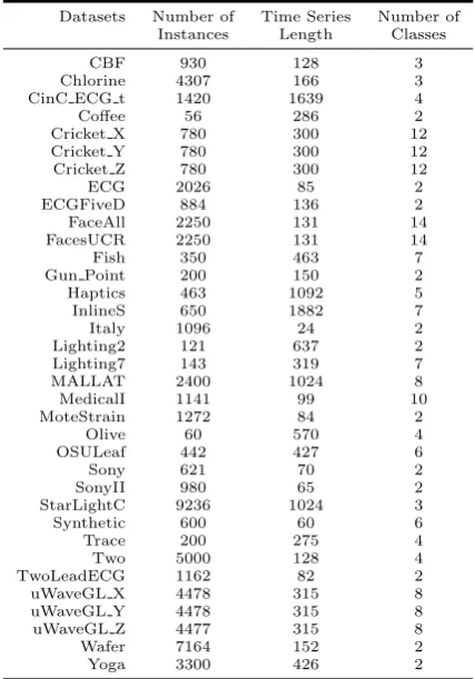
The experimentation is based on 35 standard classification datasets taken from public available repositories (Chen et al., 2015; Wei, 2006). Table 2 summarizes the main properties of the selected datasets. The datasets involved in this study contain between 56 and 9236 instances, the time series length ranges from 24 to 1882, and the number of classes varies between 2 and 14. For each dataset the time series are z-normalized, following the recommendation in Rakthanmanon et al. (2012).

The datasets are randomly divided using a 5-fold cross-validation procedure. Each training partition (4/5 of the total set of examples) is randomly divided into two sets:LandU, of labeled and unlabeled (i.e., the labels are withheld and not available to the algorithm) examples, respectively. Following the approach of Triguero et al. (2015) and Wang et al. (2010), we do not attempt to keep the class proportion in theLandU sets the same as in the whole training set. The class label of the instances selected to form the setU is removed. We make sure that every class has been represented inL.

(8)

Datasets Number of Time Series Number of Instances Length Classes

CBF 930 128 3

Chlorine 4307 166 3

CinC ECG t 1420 1639 4

Coffee 56 286 2

Cricket X 780 300 12

Cricket Y 780 300 12

Cricket Z 780 300 12

ECG 2026 85 2

ECGFiveD 884 136 2

FaceAll 2250 131 14

FacesUCR 2250 131 14

Fish 350 463 7

Gun Point 200 150 2

Haptics 463 1092 5

InlineS 650 1882 7

Italy 1096 24 2

Lighting2 121 637 2

Lighting7 143 319 7

MALLAT 2400 1024 8

MedicalI 1141 99 10

MoteStrain 1272 84 2

Olive 60 570 4

OSULeaf 442 427 6

Sony 621 70 2

SonyII 980 65 2

StarLightC 9236 1024 3

Synthetic 600 60 6

Trace 200 275 4

Two 5000 128 4

TwoLeadECG 1162 82 2

uWaveGL X 4478 315 8

uWaveGL Y 4478 315 8

uWaveGL Z 4477 315 8

Wafer 7164 152 2

[image:8.595.162.376.130.436.2]

Yoga 3300 426 2

Table 2.Summary description of the times series datasets.

3.2. Performance measures

With the aim of measuring the effectiveness of the classification performed by the SSC techniques, we use two classical statistics: accuracy rate (Witten et al., 2011) and Cohen’s kappa rate (Ben-David, 2007). The two measures are briefly explained as follows:

– Accuracy: This measure reflects the agreement between the observed and pre-dicted classes. It is a simple metric commonly employed for assessing the per-formance of classifiers.

– Cohen’s kappa: This measure takes into account the successful hits that would be generated simply by chance. Cohen’s kappa ranges from -1 to 1, where a value of 0 means there is no agreement, a value of 1 indicates total agreement, and a negative value indicates that the prediction is in the opposite direction.

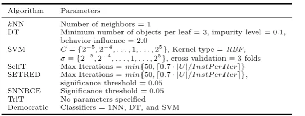
3.3. Algorithms used and parameters

(9)

Algorithm Parameters

kNN Number of neighbors = 1

DT Minimum number of objects per leaf = 3, impurity level = 0.1, behavior influence = 2.0

SVM C={2−5,2−4, . . . ,1, . . . ,25}, Kernel type =RBF,

σ={2−5,2−4, . . . ,1, . . . ,25}, cross validation = 3 folds SelfT Max Iterations =min{50,d0.7· |U|/InstP erItere}

SETRED Max Iterations =min{50,d0.7· |U|/InstP erItere}, significance threshold = 0.05

[image:9.595.126.424.127.240.2]

SNNRCE Significance threshold = 0.05 TriT No parameters specified Democratic Classifiers = 1NN, DT, and SVM

Table 3. Parameter specification for the base learners and self-labeled methods involved in the experimentation.

in previous works. The parameters are not optimized for each specific dataset because the main purpose of this experimental study is to compare the gen-eral performance of the self-labeled techniques. The configuration parameters are shown in Table 3.

Some of the self-labeled methods have their own built-in stopping criteria, which we use accordingly for these methods. For classifiers which have not a predefined stopping criterion we define it as follows. For each dataset, the self-labeled process stops when it satisfies the first of the following stopping criteria: (i) 70% of the unlabeled instances in the initial setU have been removed and inserted into L or (ii) the algorithm has reached a maximum number of 50 iterations. Here,InstPerIter is the number of instances removed fromU for each iteration. The stopping criterion proposed facilitates the exploitation ofU and avoids the extreme output caused by adding in the base learner all the unlabeled instances fromU.

Most of the self-labeled methods include one or more base classifier(s). For those methods that support base classifiers from different approaches (SelfT and TriT), we explore all the possible combinations. In this study, we select as a base classifiers three methods that represent influent approaches of time series classification algorithms:kNN, DT, and SVM.

1NN is a widely used classifier in the time series classification domain. Multi-ple studies (Xing et al., 2012; Kurbalija et al., 2014; Serr`a and Arcos, 2014; Geler et al., 2015) related with time series similarity measures are based on this clas-sifier.

The method proposed in Douzal-Chouakria and Amblard (2012) is selected to construct DT specifically designed to classify time series data. This method obtains competitive results and its split procedure is flexible enough to cover behavior and value proximities. The cost functioncb to evaluate the proximity

between two series is evaluated as cb(r) = 2/(1 + exp(b·Co(r)))·c(r), where

r is a mapping between two series, Co is the behavior-based cost function, c

is the values-based cost function, and the parameter b modulates the influence of the behavior in the overall cost. This parameter has been empirically fixed to 2 (Table 3). As Co function we have used a variant of Pearson correlation involving first-order differences and asc function we have explored several time series measures.

The kernel function selected to construct the SVMs is Gaussian radial basis function (RBF), i.e.Kd(xi, xj) = exp(−d(xi, xj)2/(2σ2)). Most previous studies

(10)

combi-nation with a distance measuredselected from the time series domain. Following the methodology in Marteau and Gibet (2015), we normalize the pairwise dis-tance matrix in the training stage to limit the search space of the parameters. Specifically, we use a predefined set of C and sigma values to select the most appropriate value during a cross-validation process. Additionally, other kernels were evaluated (Shimodaira et al., 2001; Cuturi, 2011) but result of an unfeasible computational cost to be studied in the self-labeled context.

Throughout the experimentation, we evaluate five different measures to com-pute the dissimilarity between instances: Euclidean, DTW, ERP, ACF, and FFT. The Sakoe-Chiba band global constraint (Sakoe and Chiba, 1978) is used to im-prove the performance of the elastic measures. Specifically, we fix the window size to four and nine percent of the time series length for DTW and ERP, re-spectively, following the recommendation in Kurbalija et al. (2014).

4. Results and Discussion

This section presents the results obtained in the experiments and a detailed dis-cussion of those. We evaluate the performance of the methods in two different set-tings: results obtained in transductive learning (Section 4.1) and inductive learn-ing (Section 4.2), under three different ratios of labeled data. Section 4.3 presents an empirical analysis of the run-times obtained by the self-labeled techniques. Section 4.4 addresses the geometrical characteristics of the time series datasets and its influence in the performance of the techniques studied. A comparison between the supervised and semi-supervised learning paradigm is presented in Section 4.5. Finally, the discussion of all results is performed in Section 4.6.

We use non-parametric statistical tests to contrast the results obtained, fol-lowing the methodology proposed in Garc´ıa et al. (2010). Concretely, we use the Aligned Friedman test (Hodges et al., 1962) for multiple comparisons to detect statistically significant differences between the evaluated methods and

thepost-hoc procedure of Hochberg (Hochberg and Rom, 1995) to characterize

those differences. In comparisons with only two algorithms involved, we use the Wilcoxon signed rank test, following the recommendation in Demˇsar (2006).

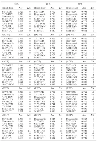
4.1. Transductive results

As stated in Section 2.1, the main goal of transductive classification is to pre-dict the class of the unlabeled data used during the training phase. Table 4 presents the average accuracy (Acc) results of the self-labeled methods involved in this study over the 35 datasets with 10%, 20%, and 30% of labeled data. The methods are presented in descending order of the accuracy. For those methods that support different base classifiers, we have explored all possible combinations specifying the classifier in the method’s name.

(11)

10% 20% 30%

(Euclidean) Acc ∆K (Euclidean) Acc ∆K (Euclidean) Acc ∆K

SETRED 0.720 0 SETRED 0.762 0 SETRED 0.794 0

TriT-1NN 0.718 0 Democratic 0.760 0 Democratic 0.793 0 Democratic 0.715 0 TriT-1NN 0.759 0 TriT-1NN 0.790 0 SelfT-1NN 0.708 0 SelfT-1NN 0.750 0 SNNRCE 0.781 -2 SNNRCE 0.707 0 SNNRCE 0.749 0 TriT-SVM 0.777 +1 TriT-SVM 0.694 0 TriT-SVM 0.734 0 SelfT-1NN 0.776 +1 TriT-DT 0.635 0 SelfT-SVM 0.686 0 SelfT-SVM 0.721 0 SelfT-SVM 0.618 0 TriT-DT 0.671 0 TriT-DT 0.694 0 SelfT-DT 0.598 0 SelfT-DT 0.639 0 SelfT-DT 0.664 0

(DTW) Acc ∆K (DTW) Acc ∆K (DTW) Acc ∆K

TriT-1NN 0.771 0 TriT-1NN 0.815 0 TriT-1NN 0.840 0

Democratic 0.758 0 Democratic 0.802 0 Democratic 0.829 0

SNNRCE 0.757 0 SNNRCE 0.800 0 SNNRCE 0.827 0

SelfT-1NN 0.745 0 SelfT-1NN 0.787 0 SelfT-1NN 0.812 0 TriT-SVM 0.732 0 TriT-SVM 0.782 0 TriT-SVM 0.806 0 TriT-DT 0.679 0 TriT-DT 0.718 -1 SelfT-SVM 0.750 0 SelfT-DT 0.638 -1 SelfT-SVM 0.715 +1 TriT-DT 0.748 0 SelfT-SVM 0.638 +1 SelfT-DT 0.681 0 SelfT-DT 0.710 0

(ACF) Acc ∆K (ACF) Acc ∆K (ACF) Acc ∆K

Democratic 0.677 0 Democratic 0.709 0 Democratic 0.730 0 SelfT-1NN 0.655 0 SelfT-1NN 0.687 0 TriT-DT 0.708 -1 TriT-DT 0.654 0 TriT-DT 0.684 0 SelfT-1NN 0.705 +1 TriT-SVM 0.640 0 TriT-SVM 0.683 0 TriT-SVM 0.699 -1 SelfT-DT 0.627 0 SelfT-DT 0.665 0 SelfT-DT 0.693 +1 SelfT-SVM 0.569 0 SelfT-SVM 0.632 0 SelfT-SVM 0.659 0

(FFT) Acc ∆K (FFT) Acc ∆K (FFT) Acc ∆K

SETRED 0.721 0 SETRED 0.762 0 SETRED 0.794 -1 Democratic 0.715 0 TriT-1NN 0.760 0 Democratic 0.794 +1 TriT-1NN 0.715 0 Democratic 0.759 0 TriT-1NN 0.790 0 SelfT-1NN 0.709 0 SNNRCE 0.750 -1 SNNRCE 0.782 -1 SNNRCE 0.708 0 SelfT-1NN 0.749 +1 SelfT-1NN 0.776 +1 TriT-SVM 0.694 0 TriT-SVM 0.741 0 TriT-SVM 0.768 0 TriT-DT 0.636 0 SelfT-SVM 0.681 0 SelfT-SVM 0.723 0 SelfT-SVM 0.622 0 TriT-DT 0.673 0 TriT-DT 0.696 0 SelfT-DT 0.597 0 SelfT-DT 0.639 0 SelfT-DT 0.663 0

(ERP) Acc ∆K (ERP) Acc ∆K (ERP) Acc ∆K

[image:11.595.107.433.124.596.2]

SETRED 0.783 0 Democratic 0.825 0 Democratic 0.847 0 Democratic 0.780 0 TriT-1NN 0.821 0 TriT-1NN 0.846 0 TriT-1NN 0.779 0 SETRED 0.820 0 SETRED 0.845 0 TriT-SVM 0.772 0 SNNRCE 0.808 0 TriT-SVM 0.836 0 SNNRCE 0.767 -1 TriT-SVM 0.805 -1 SNNRCE 0.832 0 SelfT-1NN 0.760 +1 SelfT-1NN 0.800 +1 SelfT-1NN 0.823 0 SelfT-SVM 0.724 0 TriT-DT 0.736 0 TriT-DT 0.762 -1 TriT-DT 0.696 0 SelfT-SVM 0.722 0 SelfT-SVM 0.756 +1 SelfT-DT 0.689 0 SelfT-DT 0.697 0 SelfT-DT 0.722 0

(12)

0.2

0.4

0.6

0.8

1.0

accur

acy

SelfT−1NN SETRED SNNRCE T

riT−1NN

Democr

atic

SelfT−SVM T

riT−SVM SelfT−DT T

riT−DT

ACF DTW ERP Euc FFT

(a)

0.2

0.4

0.6

0.8

1.0

accur

acy

riT−1NN

Democr

atic

SelfT−SVM T

riT−DT

ACF DTW ERP Euc FFT

(b)

0.2

0.4

0.6

0.8

1.0

accur

acy

riT−1NN

Democr

atic

SelfT−SVM T

riT−DT

ACF DTW ERP Euc FFT

[image:12.595.108.422.147.423.2]

(c)

Figure 1. Box and whisker plots for the accuracy in transductive phase. The bottom and top of a box are the first and third quartiles. The band inside the box is the median. (a) 10% labeled data. (b) 20% labeled data. (c) 30% labeled data.

Figure 1 shows box and whisker plots of the methods under the dissimilarity measures studied. This illustration allows us to visualize in more detail the per-formance of the self-labeled methods. It shows the gain of accuracy caused by the use of DTW and ERP in comparison with the other measures. The superiority of DTW over Euclidean distance has been addressed in previous studies about time series classification problem. For instance, the extensive study performed by Serr`a and Arcos (2014) supports this conclusion. Furthermore, the study of Wang et al. (2013) reveals that DTW and ERP are clearly superior to Eucli-den distance. In this sense, our results confirm the advantage of these elastic measures in the semi-supervised context.

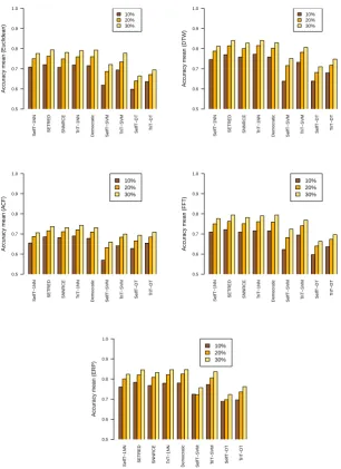
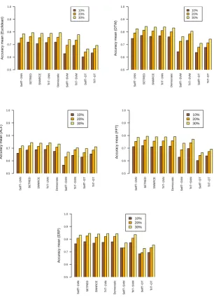
On the other hand, the methods combined with 1NN as a base classifier exhibit the better performance. By contrast, the lowest results are obtained in combination with DT. Moreover, the use of SVM as a base classifier causes a spread behavior of the accuracy values. Figure 2 presents the average results in a bar plot aiming to compare the accuracy values across different labeled ratios. We perform a comparison of the accuracy among all single learning methods grouped by their learning scheme. This comparison allows us to determine the most successful self-labeled methods for each base classifier.

(13)

riT−1NN

Democr

atic

SelfT−SVM T

riT−DT

10% 20% 30%

Accur

acy mean (Euclidean)

0.5 0.6 0.7 0.8 0.9 1.0

riT−1NN

Democr

atic

SelfT−SVM T

riT−DT

10% 20% 30%

Accur

acy mean (DTW)

0.5 0.6 0.7 0.8 0.9 1.0

riT−1NN

Democr

atic

SelfT−SVM T

riT−DT

10% 20% 30%

Accur

acy mean (A

CF)

0.5 0.6 0.7 0.8 0.9 1.0

riT−1NN

Democr

atic

SelfT−SVM T

riT−DT

10% 20% 30%

Accur

acy mean (FFT)

0.5 0.6 0.7 0.8 0.9 1.0

riT−1NN

Democr

atic

SelfT−SVM T

riT−DT

10% 20% 30%

Accur

acy mean (ERP)

[image:13.595.110.417.148.570.2]

0.5 0.6 0.7 0.8 0.9 1.0

Figure 2. Bar plot of the comparison between the average accuracy obtained during the transductive phase.

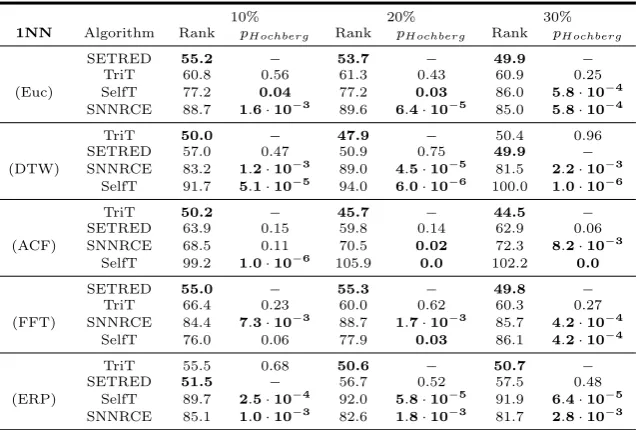
1NN as a base classifier, detects significant differences on a significance level of

(14)

val-10% 20% 30%

1NN Algorithm Rank pHochberg Rank pHochberg Rank pHochberg

SETRED 55.2 − 53.7 − 49.9 −

TriT 60.8 0.56 61.3 0.43 60.9 0.25

(Euc) SelfT 77.2 0.04 77.2 0.03 86.0 5.8·10−4

SNNRCE 88.7 1.6·10−3 89.6 6.4·10−5 85.0 5.8·10−4

TriT 50.0 − 47.9 − 50.4 0.96

SETRED 57.0 0.47 50.9 0.75 49.9 −

(DTW) SNNRCE 83.2 1.2·10−3 _89.0 ₄_.₅_·₁₀−5 _81.5 ₂_.₂_·₁₀−3 SelfT 91.7 5.1·10−5 _94.0 ₆_.₀_·₁₀−6 _100.0 ₁_.₀_·₁₀−6

TriT 50.2 − 45.7 − 44.5 −

SETRED 63.9 0.15 59.8 0.14 62.9 0.06

(ACF) SNNRCE 68.5 0.11 70.5 0.02 72.3 8.2·10−3

SelfT 99.2 1.0·10−6 105.9 0.0 102.2 0.0

SETRED 55.0 − 55.3 − 49.8 −

TriT 66.4 0.23 60.0 0.62 60.3 0.27

(FFT) SNNRCE 84.4 7.3·10−3 _88.7 ₁_.₇_·₁₀−3 _85.7 ₄_.₂_·₁₀−4 SelfT 76.0 0.06 77.9 0.03 86.1 4.2·10−4

TriT 55.5 0.68 50.6 − 50.7 −

SETRED 51.5 − 56.7 0.52 57.5 0.48

(ERP) SelfT 89.7 2.5·10−4 92.0 5.8·10−5 91.9 6.4·10−5

[image:14.595.111.431.129.344.2]

SNNRCE 85.1 1.0·10−3 _82.6 ₁_.₈_·₁₀−3 _81.7 ₂_.₈_·₁₀−3

Table 5.Aligned Friedman ranking of the accuracy using 1NN as a base classifier. Adjusted

p-values for thepost-hocprocedure of Hochberg.

10% 20% 30%

DT Algorithms Neg Pos pvalue Neg Pos pvalue Neg Pos pvalue

(Euc) TriT−SelfT 4 31 4.0·10−6 4 31 1.0·10−5 3 32 1.0·10−6

(DTW) TriT−SelfT 3 32 1.0·10−6 5 30 2.0·10−6 1 34 0.0

(ACF) TriT−SelfT 9 26 8.0·10−3 10 25 7.0·10−3 8 27 6.0·10−3

(FFT) TriT−SelfT 5 30 2.0·10−6 3 32 2.0·10−6 3 32 1.0·10−6

(ERP) TriT−SelfT 16 19 0.53 2 33 1.0·10−6 2 33 0.0

10% 20% 30%

SVM Algorithms Neg Pos pvalue Neg Pos pvalue Neg Pos pvalue

(Euc) TriT−SelfT 5 30 7.0·10−6 12 23 4.0·10−3 8 27 1.0·10−4

(DTW) TriT−SelfT 5 30 3.0·10−6 ₈ ₂₇ ₃_.₂_·₁₀−5 ₇ ₂₈ ₂_.₁_·₁₀−5 (ACF) TriT−SelfT 9 26 2.7·10−4 ₆ ₂₉ ₂_.₂_·₁₀−4 ₁₂ ₂₃ ₃_.₀_·₁₀−3 (FFT) TriT−SelfT 7 28 5.0·10−6 ₈ ₂₇ ₃_.₁_·₁₀−4 ₁₀ ₂₅ ₂_.₈_·₁₀−3 (ERP) TriT−SelfT 16 19 0.09 5 30 2.1·10−5 ₇ ₂₆ ₁_.₄_·₁₀−4

Table 6.Wilcoxon Signed Ranks Test of the accuracy for DT and SVM as a base classifiers. The number of negative and positive ranks is showed in conjunction with thep-value.

ues of accuracy. In the majority of comparisons, these methods are significantly outperformed by the control method, following the Hochbergpost-hocprocedure. Table 6 shows the application of the Wilcoxon Signed Ranks Test to contrast the accuracy of the methods that use DT and SVM as a base classifiers. For all dissimilarity measures and labeled ratios, TriT outperforms SelfT using both base classifiers. The difference obtained results significant on a significance level ofα= 0.05, with the exception of ERP at 10% of labeled data.

(15)

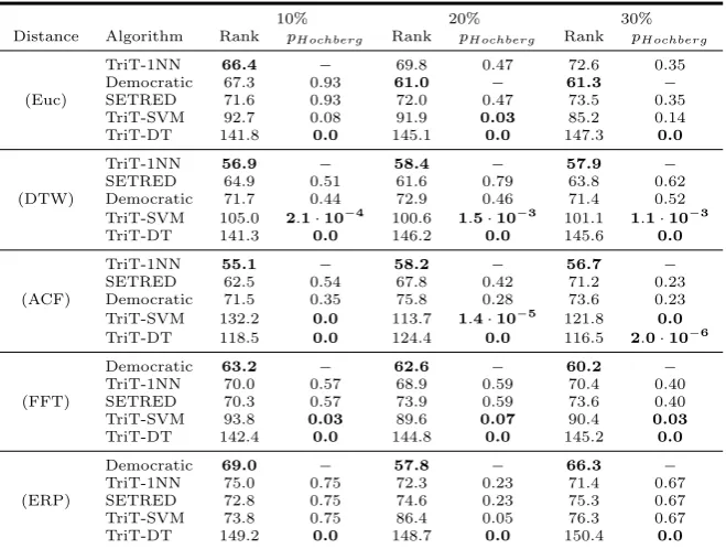
10% 20% 30% Distance Algorithm Rank pHochberg Rank pHochberg Rank pHochberg

TriT-1NN 66.4 − 69.8 0.47 72.6 0.35

Democratic 67.3 0.93 61.0 − 61.3 −

(Euc) SETRED 71.6 0.93 72.0 0.47 73.5 0.35

TriT-SVM 92.7 0.08 91.9 0.03 85.2 0.14

TriT-DT 141.8 0.0 145.1 0.0 147.3 0.0

TriT-1NN 56.9 − 58.4 − 57.9 −

SETRED 64.9 0.51 61.6 0.79 63.8 0.62

(DTW) Democratic 71.7 0.44 72.9 0.46 71.4 0.52 TriT-SVM 105.0 2.1·10−4 100.6 1.5·10−3 101.1 1.1·10−3

TriT-DT 141.3 0.0 146.2 0.0 145.6 0.0

TriT-1NN 55.1 − 58.2 − 56.7 −

SETRED 62.5 0.54 67.8 0.42 71.2 0.23

(ACF) Democratic 71.5 0.35 75.8 0.28 73.6 0.23 TriT-SVM 132.2 0.0 113.7 1.4·10−5 _121.8 _0.0 TriT-DT 118.5 0.0 124.4 0.0 116.5 2.0·10−6

Democratic 63.2 − 62.6 − 60.2 −

TriT-1NN 70.0 0.57 68.9 0.59 70.4 0.40

(FFT) SETRED 70.3 0.57 73.9 0.59 73.6 0.40

TriT-SVM 93.8 0.03 89.6 0.07 90.4 0.03

TriT-DT 142.4 0.0 144.8 0.0 145.2 0.0

Democratic 69.0 − 57.8 − 66.3 −

TriT-1NN 75.0 0.75 72.3 0.23 71.4 0.67

(ERP) SETRED 72.8 0.75 74.6 0.23 75.3 0.67

TriT-SVM 73.8 0.75 86.4 0.05 76.3 0.67

[image:15.595.105.435.129.378.2]

TriT-DT 149.2 0.0 148.7 0.0 150.4 0.0

Table 7.Aligned Friedman ranking of the accuracy of the most competent methods for each learning approach using the dissimilarity measures studied. Adjustedp-values for thepost-hoc

procedure of Hochberg.

three labeled ratios) in Tables 5 and 6. Following this criterion the outstanding methods selected are: SETRED and TriT.

The Aligned Friedman test, applied to accuracy, detects significant differences on a significance level of α = 0.05 for all comparisons performed. For the dis-similarity measures DTW and ACF, the control method selected is TriT-1NN in most cases. For the dissimilarity measures Euclidean, FFT and ERP, Democratic is selected as control method in most of the comparisons. SETRED exhibits a competitive behavior because is not outperformed by the control method in any of comparisons. By contrast, TriT-SVM and TriT-DT are significantly outper-formed by the control method in most of the comparisons peroutper-formed, with the exception of ERP where TriT-SVM exhibits a better behavior.

4.2. Inductive results

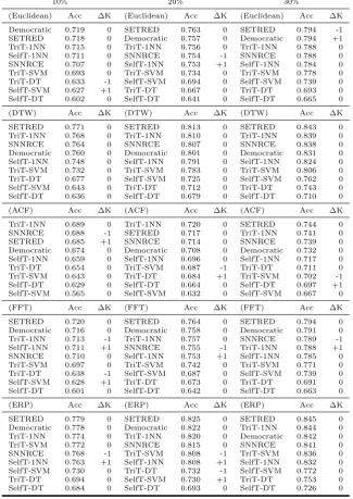
The main target of inductive learning is to classify instances not included in the training phase. This analysis is useful to test the previous learned hypothe-ses and their generalization abilities. Table 8 shows the average obtained using all dissimilarity measures studied. Figure 4 shows box and whisker plots of the same results grouped by ratios. Figure 3 shows a bar plot of the average accu-racy reflecting the improvement obtained by increasing the amount of labeled examples.

(16)

10% 20% 30%

(Euclidean) Acc ∆K (Euclidean) Acc ∆K (Euclidean) Acc ∆K

Democratic 0.719 0 SETRED 0.763 0 SETRED 0.794 -1 SETRED 0.718 0 Democratic 0.757 0 Democratic 0.794 +1 TriT-1NN 0.715 0 TriT-1NN 0.756 0 TriT-1NN 0.788 0 SelfT-1NN 0.711 0 SNNRCE 0.754 -1 SNNRCE 0.788 0 SNNRCE 0.707 0 SelfT-1NN 0.753 +1 SelfT-1NN 0.784 0 TriT-SVM 0.693 0 TriT-SVM 0.734 0 TriT-SVM 0.778 0 TriT-DT 0.633 -1 SelfT-SVM 0.694 0 SelfT-SVM 0.739 0 SelfT-SVM 0.627 +1 TriT-DT 0.667 0 TriT-DT 0.693 0 SelfT-DT 0.602 0 SelfT-DT 0.641 0 SelfT-DT 0.665 0

(DTW) Acc ∆K (DTW) Acc ∆K (DTW) Acc ∆K

Democratic 0.760 0 Democratic 0.801 0 Democratic 0.831 0 SelfT-1NN 0.748 0 SelfT-1NN 0.791 0 SelfT-1NN 0.824 0 TriT-SVM 0.732 0 TriT-SVM 0.783 0 TriT-SVM 0.806 0 TriT-DT 0.677 0 SelfT-SVM 0.725 0 SelfT-SVM 0.762 0 SelfT-SVM 0.643 0 TriT-DT 0.712 0 TriT-DT 0.743 0 SelfT-DT 0.636 0 SelfT-DT 0.679 0 SelfT-DT 0.710 0

(ACF) Acc ∆K (ACF) Acc ∆K (ACF) Acc ∆K

TriT-1NN 0.689 0 TriT-1NN 0.720 0 SETRED 0.744 0 SNNRCE 0.688 -1 SETRED 0.717 0 TriT-1NN 0.741 0 SETRED 0.685 +1 SNNRCE 0.714 0 SNNRCE 0.739 0 Democratic 0.674 0 Democratic 0.708 0 Democratic 0.732 0 SelfT-1NN 0.659 0 SelfT-1NN 0.696 0 SelfT-1NN 0.717 0 TriT-DT 0.654 0 TriT-SVM 0.687 -1 TriT-DT 0.711 0 TriT-SVM 0.643 0 TriT-DT 0.684 +1 TriT-SVM 0.702 -1 SelfT-DT 0.629 0 SelfT-DT 0.664 0 SelfT-DT 0.697 +1 SelfT-SVM 0.565 0 SelfT-SVM 0.632 0 SelfT-SVM 0.667 0

(FFT) Acc ∆K (FFT) Acc ∆K (FFT) Acc ∆K

Democratic 0.716 0 Democratic 0.758 0 Democratic 0.791 0 TriT-1NN 0.713 -1 TriT-1NN 0.757 0 SNNRCE 0.789 -1 SelfT-1NN 0.711 +1 SNNRCE 0.755 -1 TriT-1NN 0.788 +1 SNNRCE 0.710 0 SelfT-1NN 0.753 +1 SelfT-1NN 0.785 0 TriT-SVM 0.697 0 TriT-SVM 0.742 0 TriT-SVM 0.771 0 TriT-DT 0.638 -1 SelfT-SVM 0.687 0 SelfT-SVM 0.739 0 SelfT-SVM 0.628 +1 TriT-DT 0.673 0 TriT-DT 0.691 0 SelfT-DT 0.601 0 SelfT-DT 0.642 0 SelfT-DT 0.663 0

(ERP) Acc ∆K (ERP) Acc ∆K (ERP) Acc ∆K

[image:16.595.107.433.136.596.2]

Democratic 0.778 0 Democratic 0.822 0 TriT-1NN 0.844 0 TriT-1NN 0.774 0 TriT-1NN 0.820 0 Democratic 0.842 0 TriT-SVM 0.772 0 SNNRCE 0.815 0 SNNRCE 0.841 0 SNNRCE 0.768 -1 TriT-SVM 0.808 -1 TriT-SVM 0.836 0 SelfT-1NN 0.763 +1 SelfT-1NN 0.808 +1 SelfT-1NN 0.832 0 SelfT-SVM 0.730 0 TriT-DT 0.732 -1 SelfT-SVM 0.772 0 TriT-DT 0.694 0 SelfT-SVM 0.730 +1 TriT-DT 0.753 0 SelfT-DT 0.684 0 SelfT-DT 0.693 0 SelfT-DT 0.726 0

(17)

riT−1NN

Democr

atic

SelfT−SVM T

riT−DT

10% 20% 30%

Accur

acy mean (Euclidean)

0.5 0.6 0.7 0.8 0.9 1.0

riT−1NN

Democr

atic

SelfT−SVM T

riT−DT

10% 20% 30%

Accur

acy mean (DTW)

0.5 0.6 0.7 0.8 0.9 1.0

riT−1NN

Democr

atic

SelfT−SVM T

riT−DT

10% 20% 30%

Accur

acy mean (A

CF)

0.5 0.6 0.7 0.8 0.9 1.0

riT−1NN

Democr

atic

SelfT−SVM T

riT−DT

10% 20% 30%

Accur

acy mean (FFT)

0.5 0.6 0.7 0.8 0.9 1.0

riT−1NN

Democr

atic

SelfT−SVM T

riT−DT

10% 20% 30%

Accur

acy mean (ERP)

[image:17.595.110.417.146.572.2]

0.5 0.6 0.7 0.8 0.9 1.0

Figure 3. Bar plot of the comparison between the average accuracy obtained during the transductive phase.

(18)

0.2

0.4

0.6

0.8

1.0

accur

acy

riT−1NN

Democr

atic

SelfT−SVM T

riT−DT

ACF DTW ERP Euc FFT

(a)

0.2

0.4

0.6

0.8

1.0

accur

acy

riT−1NN

Democr

atic

SelfT−SVM T

riT−DT

ACF DTW ERP Euc FFT

(b)

0.2

0.4

0.6

0.8

1.0

accur

acy

riT−1NN

Democr

atic

SelfT−SVM T

riT−DT

ACF DTW ERP Euc FFT

[image:18.595.100.458.150.467.2]

(c)

Figure 4. Box and whisker plots for the accuracy in inductive phase. (a) 10% labeled data. (b) 20% labeled data. (c) 30% labeled data.

by the control method in most of the comparisons following the Hochberg post-hoc procedure.

Table 10 shows the application of the Wilcoxon Signed Ranks Test to the accuracy for the methods that use DT and SVM as a base classifiers. For all dissimilarity measures and labeled ratios, TriT outperforms significantly SelfT using both base classifiers, with the exception of SVM under ERP at 10% of labeled data.

(19)

out-10% 20% 30%

1NN Algorithm Rank pHochberg Rank pHochberg Rank pHochberg

SETRED 56.7 − 53.5 − 53.3 −

TriT 67.2 0.27 72.5 0.06 68.4 0.04

(Euc) SelfT 69.4 0.27 76.2 0.04 86.2 0.03

SNNRCE 88.5 3.0·10−3 79.7 0.04 74.0 0.02

TriT 55.7 − 63.1 0.44 63.1 0.29

SETRED 58.5 0.77 55.7 − 52.9 −

(DTW) SNNRCE 72.8 0.15 73.3 0.14 73.5 0.06

SelfT 94.7 1.7·10−4 _89.8 ₁_.₃_·₁₀−3 _92.4 ₁_.₄_·₁₀−4

TriT 52.6 − 51.1 − 58.8 0.40

SETRED 68.5 0.20 61.9 0.26 50.7 −

(ACF) SNNRCE 59.8 0.45 67.9 0.16 70.0 0.09

SelfT 100.9 2.0·10−6 101.0 1.0·10−6 102.3 0.0

SETRED 55.4 − 53.5 − 53.9 −

TriT 72.6 0.09 73.9 0.03 68.9 0.12

(FFT) SNNRCE 82.3 0.01 78.3 0.03 73.3 0.09

SelfT 71.5 0.09 0.03 2.0·10−6 _85.8 ₃_.₀_·₁₀−3

SETRED 55.5 − 51.1 − 61.0 −

TriT 60.6 0.59 64.5 0.16 62.1 0.90

(ERP) SelfT 87.7 2.7·10−3 _89.6 ₂_.₁_·₁₀−4 _87.1 _0.02

[image:19.595.109.431.129.343.2]

SNNRCE 78.1 0.03 76.6 0.01 71.7 0.53

Table 9.Aligned Friedman ranking of the accuracy using 1NN as a base classifier. Adjusted

p-values for thepost-hocprocedure of Hochberg.

10% 20% 30%

DT Algorithms Neg Pos pvalue Neg Pos pvalue Neg Pos pvalue

(Euc) TriT−SelfT 6 28 1.3·10−5 ₆ ₂₉ ₇_.₁_·₁₀−5 ₃ ₃₂ ₅_.₀_·₁₀−6 (DTW) TriT−SelfT 3 32 2.0·10−6 ₆ ₂₉ ₁_.₀_·₁₀−5 ₃ ₃₁ ₅_.₃_·₁₀−5

(ACF) TriT−SelfT 7 27 6.7·10−3 9 26 6.8·10−3 9 26 0.01

(FFT) TriT−SelfT 4 30 1.1·10−5 4 31 3.0·10−6 5 30 6.0·10−6

(ERP) TriT−SelfT 10 24 0.04 4 30 1.0·10−6 7 28 2.0·10−4

10% 20% 30%

SVM Algorithms Neg Pos pvalue Neg Pos pvalue Neg Pos pvalue

(Euc) TriT−SelfT 6 29 2.6·10−5 12 23 8.0·10−3 9 25 1.8·10−3

(DTW) TriT−SelfT 3 32 4.0·10−6 7 27 6.1·10−5 9 26 2.2·10−4

(ACF) TriT−SelfT 6 28 1.8·10−5 7 28 2.8·10−5 10 25 3.7·10−3

(FFT) TriT−SelfT 3 32 1.0·10−6 8 27 4.0·10−4 11 23 0.01

(ERP) TriT−SelfT 15 20 0.12 4 31 6.0·10−6 ₆ ₂₇ ₁_.₀_·₁₀−4

Table 10.Wilcoxon Signed Ranks Test of the accuracy for DT and SVM as a base classifiers. The number of negative and positive ranks is showed in conjunction with thep-value.

[image:19.595.108.434.374.517.2]

(20)

10% 20% 30% Distance Algorithm Rank pHochberg Rank pHochberg Rank pHochberg

Democratic 61.0 − 63.9 − 63.2 −

SETRED 74.0 0.40 66.5 0.82 71.0 0.52

(Euc) TriT-1NN 71.0 0.40 72.5 0.82 75.8 0.52 TriT-SVM 92.3 0.02 91.7 0.02 83.6 0.27

TriT-DT 141.5 0.0 145.2 0.0 146.1 0.0

TriT-1NN 61.5 − 62.7 0.89 63.1 0.66

SETRED 65.4 0.74 61.1 − 57.9 −

(DTW) Democratic 71.5 0.74 70.6 0.86 71.4 0.52 TriT-SVM 101.7 2.7·10−3 97.5 8.0·10−3 99.6 1.7·10−3

TriT-DT 139.8 0.0 148.0 0.0 147.8 0.0

TriT-1NN 57.9 − 63.1 − 70.3 0.30

SETRED 62.3 0.71 63.3 0.98 57.8 −

(ACF) Democratic 79.5 0.14 82.4 0.22 80.4 0.12 TriT-SVM 125.4 0.0 108.3 5.6·10−4 _116.8 ₄_.₀_·₁₀−6 TriT-DT 114.7 8.0·10−6 _148.0 ₄_.₀_·₁₀−6 _147.8 ₉_.₀_·₁₀−6

Democratic 64.5 − 64.4 − 61.9 −

TriT-1NN 71.9 0.54 74.8 0.67 73.9 0.55

(FFT) SETRED 72.9 0.54 69.5 0.67 69.0 0.55

TriT-SVM 90.3 0.09 86.5 0.20 87.2 0.10

TriT-DT 140.1 0.0 144.6 0.0 147.8 0.0

Democratic 68.7 − 65.4 − 71.4 −

TriT-1NN 79.4 0.71 72.0 0.83 72.3 0.98

(ERP) SETRED 73.1 0.71 68.0 0.83 71.6 0.98

TriT-SVM 73.6 0.71 84.9 0.32 76.8 0.98

[image:20.595.107.435.129.380.2]

TriT-DT 145.0 0.0 149.5 0.0 147.7 0.0

Table 11. Aligned Friedman ranking of the accuracy of the competent methods for each learning approach using the dissimilarity measures studied. Adjustedp-values for thepost-hoc

procedure of Hochberg.

4.3. Experimental run-times

From the temporal analysis performed in Section 2.1, it is clear that the main source of temporal complexity is related with the successive operations of training the model(s) and classifying instances. The cost associated with this operations directly depends on the learning scheme(s) used. In this section, we present an empirical analysis of the run-times based on a sample of 20 datasets included in the experimentation. All experiments were performed in a cluster conformed by 46 nodes, each one equipped with an IntelrCoreTM i7-930 processor at 2.8 GHz and 24 GB of RAM memory. Under GNU/Linux we ran the experiments using R version 3.3.1 (R Core Team, 2016).

During the training and classification process, we provide the time series datasets to the self-labeled techniques using a distance matrix form. This avoids the repetitions of distance calculations and therefore it reduces the running time. For that reason the time consumption associated with the distance matrices computation are not considered in the current analysis.

(21)

Labeled %

SelfT-1NNSETRED SNNR CE

TriT-1NNDemo cratic

SelfT-SVM TriT-SVM SelfT-DT TriT-DT

[image:21.595.99.445.131.198.2]

10% 539.45 970.99 2144.17 8.67 68805.49 95584.17 16749.58 8549.26 3421.73 20% 783.28 1342.92 2139.18 8.87 90215.12 109860.63 36770.91 14051.83 3226.10 30% 960.12 1449.49 2141.10 9.17 115380.58 98829.78 54327.15 7477.80 5273.51

Table 12.Run-time means (seconds) associated with the training and testing process of the self-labeled techniques for each labeled percent evaluated.

because it trains a classifier for each learning scheme. SETRED and SNNRCE obtain competitive results as the base classifier trained is 1NN.

4.4. Impact of the geometrical characteristics of datasets

The geometrical characteristics of the datasets affect the performance of the self-labeled methods. The overlapping of samples is a common source of difficulty in the classification process. In addition, the reduced labeled sample in the SSC framework and the high dimensionality of time series data introduces another layer of complexity. In Wang et al. (2010), the overlapping of samples from different classes is investigated in order to offer an explanation of the decreasing performance experimented by the SSC algorithms in datasets that suffer this problem.

We follow a similar idea by computing the neighbors of each training instance (from U) in a neighborhood graph constructed from L∪U. The proportion of neighbors (from L) with a different class with respect to the training instance analyzed, is used as an overlapping measure. Table 13 includes this overlapping measured averaged for all training examples of each dataset. The neighborhood graph was computed for each dissimilarity measure and proportion of labeled data. The datasets with high proportions of neighbors with different class are related with high levels of overlap between classes.

In order to investigate the impact of the overlapping in the classification performance, we correlate the values of Table 13 with the accuracy obtained with the self-labeled techniques. Figure 5 shows the correlations obtained between the two variables studied (accuracy and overlapping). For all dissimilarity measures and proportions of labeled data studied, both variables present an strong inverse correlation. This means that the presence of overlapping in datasets affects, in a significant manner, the performance of the self-labeled techniques.

Considering the impact of overlapping in the techniques performance, we present a study about the tunning of some parameters based on the level of overlapping in the datasets. Specifically, we study the parameter significance threshold that controls the addition mechanism in the methods SETRED and SNNRCE. In the case of SETRED, this parameter controls the hypothesis used to decide if an specific example must be added or not to the labeled set L. The smaller this value, the more restrictive the selection of examples that are considered good is. In the case of SNNRCE, the significance threshold is related with the hypothesis used to determine if an example is considered as a “doubt example”. The greater this value, the more examples will be considered as doubt and accordingly to the SNNRCE method they will be relabeled.

(22)

Datasets _10% _20%Euc _30% _10% DTW_20% _30% _10% ACF_20% _30% _10% FFT_20% _30% _10% ERP_20% _30%

CBF 0.18 0.14 0.11 0.12 0.08 0.06 0.26 0.22 0.20 0.18 0.14 0.11 0.08 0.05 0.04 Chlorine 0.49 0.43 0.38 0.50 0.45 0.40 0.51 0.46 0.41 0.49 0.43 0.38 0.50 0.45 0.39 CinC ECG t 0.18 0.12 0.08 0.17 0.11 0.09 0.20 0.15 0.12 0.18 0.12 0.08 0.23 0.14 0.12 Coffee 0.21 0.18 0.13 0.28 0.16 0.19 0.31 0.28 0.16 0.21 0.18 0.13 0.26 0.19 0.17 Cricket X 0.77 0.71 0.66 0.70 0.63 0.58 0.71 0.64 0.61 0.77 0.71 0.66 0.66 0.57 0.52

Cricket Y 0.75 0.69 0.66 0.69 0.61 0.57 0.71 0.66 0.63 0.75 0.69 0.66 0.63 0.54 0.50

Cricket Z 0.77 0.69 0.66 0.71 0.62 0.59 0.69 0.63 0.60 0.77 0.69 0.66 0.67 0.56 0.52

ECG 0.06 0.04 0.03 0.06 0.05 0.04 0.08 0.05 0.04 0.06 0.04 0.03 0.05 0.04 0.03 ECGFiveD 0.18 0.14 0.12 0.20 0.16 0.14 0.07 0.05 0.03 0.18 0.14 0.12 0.19 0.14 0.11 FaceAll 0.46 0.36 0.33 0.31 0.24 0.22 0.43 0.35 0.32 0.46 0.36 0.33 0.28 0.22 0.20 FacesUCR 0.47 0.37 0.33 0.32 0.25 0.22 0.43 0.35 0.31 0.47 0.37 0.33 0.28 0.22 0.20 Fish 0.53 0.46 0.40 0.52 0.44 0.40 0.55 0.49 0.46 0.53 0.46 0.40 0.49 0.41 0.35 Gun Point 0.35 0.27 0.21 0.25 0.19 0.14 0.28 0.23 0.19 0.35 0.27 0.21 0.26 0.19 0.15 Haptics 0.67 0.67 0.65 0.68 0.67 0.64 0.68 0.68 0.67 0.67 0.67 0.65 0.66 0.63 0.62

InlineS 0.78 0.74 0.70 0.76 0.70 0.65 0.79 0.75 0.73 0.78 0.74 0.70 0.71 0.64 0.59

Italy 0.06 0.05 0.05 0.09 0.08 0.08 0.12 0.09 0.09 0.06 0.05 0.05 0.11 0.08 0.08 Lighting2 0.41 0.39 0.42 0.35 0.34 0.30 0.35 0.34 0.33 0.41 0.39 0.42 0.37 0.32 0.29 Lighting7 0.66 0.60 0.58 0.60 0.48 0.45 0.55 0.53 0.49 0.66 0.60 0.58 0.57 0.46 0.41 MALLAT 0.10 0.08 0.07 0.11 0.08 0.07 0.12 0.09 0.08 0.10 0.08 0.07 0.15 0.12 0.10 MedicalI 0.51 0.45 0.41 0.52 0.44 0.40 0.56 0.48 0.44 0.51 0.45 0.41 0.49 0.41 0.39 MoteStrain 0.14 0.14 0.14 0.13 0.11 0.10 0.25 0.23 0.22 0.14 0.14 0.14 0.13 0.11 0.11 Olive 0.34 0.33 0.25 0.34 0.32 0.27 0.40 0.37 0.30 0.34 0.33 0.25 0.38 0.33 0.27 OSULeaf 0.67 0.62 0.59 0.67 0.61 0.58 0.51 0.46 0.45 0.67 0.62 0.59 0.65 0.59 0.55

[image:22.595.103.437.127.362.2]

Sony 0.16 0.12 0.09 0.16 0.13 0.11 0.15 0.12 0.11 0.16 0.12 0.09 0.13 0.11 0.09 SonyII 0.16 0.13 0.10 0.18 0.14 0.13 0.17 0.13 0.11 0.16 0.13 0.10 0.16 0.13 0.12 StarLightC 0.17 0.15 0.14 0.13 0.11 0.10 0.11 0.10 0.09 0.17 0.15 0.14 0.14 0.13 0.12 Synthetic 0.41 0.35 0.31 0.32 0.24 0.22 0.41 0.39 0.37 0.41 0.35 0.32 0.20 0.16 0.14 Trace 0.49 0.50 0.48 0.39 0.33 0.26 0.36 0.31 0.26 0.49 0.50 0.48 0.35 0.34 0.32 Two 0.53 0.48 0.45 0.40 0.34 0.31 0.55 0.53 0.52 0.53 0.48 0.45 0.25 0.20 0.17 TwoLeadECG 0.19 0.13 0.10 0.12 0.09 0.08 0.11 0.09 0.09 0.19 0.13 0.10 0.07 0.05 0.05 uWaveGL X 0.40 0.36 0.34 0.39 0.36 0.33 0.56 0.55 0.53 0.40 0.36 0.34 0.37 0.34 0.32 uWaveGL Y 0.44 0.41 0.39 0.44 0.41 0.39 0.66 0.64 0.63 0.44 0.41 0.39 0.44 0.42 0.40 uWaveGL Z 0.45 0.41 0.40 0.44 0.40 0.38 0.55 0.53 0.52 0.45 0.41 0.40 0.42 0.38 0.37 Wafer 0.02 0.01 0.01 0.02 0.02 0.01 0.02 0.02 0.01 0.02 0.01 0.01 0.03 0.02 0.01 Yoga 0.26 0.21 0.17 0.24 0.19 0.16 0.27 0.22 0.21 0.26 0.21 0.17 0.24 0.19 0.16

Table 13.The proportions of neighbors with different class computed for each training in-stance, using the information provided by a neighborhood graph. The values highest than 0.5 were highlighted.

throughout different levels of overlap. The significance threshold selected is the value, between three possible values (0.05, 0.10, and 0.15), that maximizes the accuracy of SETRED. In general, the most appropriated threshold for datasets seems to be the most restrictive value 0.05. This value benefits datasets with low overlapping. For other datasets, including those with medium or high degree of overlap are more flexible values of significance threshold preferred. This behavior is more noticeable at 30% of labeled data.

(23)

−0.92 −0.9 −0.9 −0.94 −0.94 −0.93 −0.93 −0.93 −0.95 −0.91 −0.9 −0.9 −0.9 −0.88 −0.9 −0.92 −0.92 −0.92 −0.9 −0.91 −0.91 −0.87 −0.86 −0.86 −0.87 −0.87 −0.85 −0.89 −0.94 −0.94 −0.87 −0.86 −0.85 −0.88 −0.88 −0.86 −0.9 −0.91 −0.91 −0.87 −0.86 −0.86 −0.87 −0.87 −0.85

Euc DTW ACF FFT ERP

SelfT−1NN SelfT−DT SelfT−SVM SETRED SNNRCE TriT−1NN TriT−DT TriT−SVM Democratic

(a) 10% labeled

−0.93 −0.91 −0.91 −0.94 −0.95 −0.94 −0.94 −0.94 −0.95 −0.88 −0.9 −0.9 −0.88 −0.88 −0.87 −0.89 −0.89 −0.89 −0.98 −0.95 −0.95 −0.98 −0.96 −0.96 −0.95 −0.95 −0.96 −0.93 −0.91 −0.91 −0.94 −0.95 −0.94 −0.95 −0.95 −0.96 −0.89 −0.9 −0.9 −0.88 −0.89 −0.88 −0.89 −0.89 −0.9

Euc DTW ACF FFT ERP

(b) 20% labeled

−0.92 −0.93 −0.93 −0.92 −0.94 −0.93 −0.95 −0.95 −0.95 −0.84 −0.9 −0.9 −0.85 −0.85 −0.85 −0.88 −0.88 −0.88 −0.96 −0.96 −0.96 −0.97 −0.97 −0.97 −0.96 −0.96 −0.96 −0.92 −0.91 −0.91 −0.92 −0.94 −0.93 −0.94 −0.94 −0.94 −0.89 −0.9 −0.9 −0.89 −0.86 −0.89 −0.88 −0.88 −0.91

Euc DTW ACF FFT ERP

[image:23.595.127.434.127.505.2]

(c) 30% labeled

(24)

0.0 0.2 0.4 0.6 0.8

Overlapping degree

Significance threshold

5

10

15

(a) Euclidean 10%

0.0 0.2 0.4 0.6 0.8

Overlapping degree

5

10

15

(b) Euclidean 20%

0.0 0.2 0.4 0.6 0.8

Overlapping degree

5

10

15

(c) Euclidean 30%

0.0 0.2 0.4 0.6 0.8

Overlapping degree

5

10

15

(d) DTW 10%

0.0 0.2 0.4 0.6 0.8

Overlapping degree

5

10

15

(e) DTW 20%

0.0 0.2 0.4 0.6 0.8

Overlapping degree

5

10

15

(f) DTW 30%

0.0 0.2 0.4 0.6 0.8

Overlapping degree

5

10

15

(g) ACF 10%

0.0 0.2 0.4 0.6 0.8

Overlapping degree

5

10

15

(h) ACF 20%

0.0 0.2 0.4 0.6 0.8

Overlapping degree

5

10

15

[image:24.595.102.427.143.538.2]

(i) ACF 30%

(25)

0.0 0.2 0.4 0.6 0.8

Overlapping degree

5

10

15

(a) FFT 10%

0.0 0.2 0.4 0.6 0.8

Overlapping degree

5

10

15

(b) FFT 20%

0.0 0.2 0.4 0.6 0.8

Overlapping degree

5

10

15

(c) FFT 30%

0.0 0.2 0.4 0.6 0.8

Overlapping degree

5

10

15

(d) ERP 10%

0.0 0.2 0.4 0.6 0.8

Overlapping degree

5

10

15

(e) ERP 20%

0.0 0.2 0.4 0.6 0.8

Overlapping degree

5

10

15

[image:25.595.105.426.150.401.2]

(f) ERP 30%

(26)

0.0 0.2 0.4 0.6 0.8

Overlapping degree

5

10

15

(a) Euclidean 10%

0.0 0.2 0.4 0.6 0.8

Overlapping degree

5

10

15

(b) Euclidean 20%

0.0 0.2 0.4 0.6 0.8

Overlapping degree

5

10

15

(c) Euclidean 30%

0.0 0.2 0.4 0.6 0.8

Overlapping degree

5

10

15

(d) DTW 10%

0.0 0.2 0.4 0.6 0.8

Overlapping degree

5

10

15

(e) DTW 20%

0.0 0.2 0.4 0.6 0.8

Overlapping degree

5

10

15

(f) DTW 30%

0.0 0.2 0.4 0.6 0.8

Overlapping degree

5

10

15

(g) ACF 10%

0.0 0.2 0.4 0.6 0.8

Overlapping degree

5

10

15

(h) ACF 20%

0.0 0.2 0.4 0.6 0.8

Overlapping degree

5

10

15

[image:26.595.103.429.146.538.2]

(i) ACF 30%

(27)

0.0 0.2 0.4 0.6 0.8

Overlapping degree

5

10

15

(a) FFT 10%

0.0 0.2 0.4 0.6 0.8

Overlapping degree

5

10

15

(b) FFT 20%

0.0 0.2 0.4 0.6 0.8

Overlapping degree

5

10

15

(c) FFT 30%

0.0 0.2 0.4 0.6 0.8

Overlapping degree

5

10

15

(d) ERP 10%

0.0 0.2 0.4 0.6 0.8

Overlapping degree

5

10

15

(e) ERP 20%

0.0 0.2 0.4 0.6 0.8

Overlapping degree

5

10

15

[image:27.595.105.426.151.400.2]

(f) ERP 30%

(28)

4.5. Can semi-supervised learning improve classification

performance?

A recommendable procedure (Chapelle et al., 2006) in presence of labeled and unlabeled data is to start by learning a supervised classifier from the labeled data, named “baseline classifier”. A comparison with this classifier allows us to identify situations where the addition of unlabeled data causes performance degradation of the classifier obtained. In this section we perform such analysis measuring the accuracy gain obtained with the addition of unlabeled data during the training phase. We estimate the accuracy gain subtracting the accuracy obtained with supervised classification from the accuracy obtained with SSC. In both cases, the classifier performance is evaluated on the testing set, using the same 5-fold cross-validation scheme. We select as the baseline method the 1NN classifier because it offers the most accurate results.

We expect that the best-performing self-labeled methods selected from pre-vious sections will obtain the highest accuracy gain. For this reason, we focus this analysis on those methods. Figure 10 shows the accuracy gain obtained for each dataset using three semi-supervised methods. A negative gain means per-formance degradation of the classifier. We can observe a very diverse behavior of the gains under the different labeled ratios and methods. There are datasets that do not benefit from SSL, for instance ECG (Wei, 2006) and Wafer. The size of these datasets already causes that the hypothesis learned by the super-vised baseline is perfectly capable to obtain accurate classification results in the inductive phase. On other datasets, such as MedicalI, classification performance deteriorates with the addition of unlabeled data for 10% and 20% labeled ratio. This is the case as the initial labeled data provided are insufficient for training a correct model where unlabeled data will be truly beneficial. It is noticeable that MedicalI is a multi-class dataset (10 classes) with high overlapping. This adverse situation starts to reverse at 30% labeled ratio where Democratic obtains a positive accuracy difference gain.

Though there are unfavorable situations for SSL in some datasets, Figure 11 shows the gains obtained with SETRED, in decreasing order. In general, at 20% labeled data a significant positive gain can be observed. We also see that it depends heavily on the ratio of labeled instances if there is benefit and how big it is. Summarizing, the circumstances that make SSL a suitable approach for a particular dataset depend on the modeling assumptions adopted for the classifier, as well as the characteristics of the time series data.

(29)

CBF Chlor ine CinCECGt Coff ee Cr ick etX Cr ick etY Cr ick etZ _ECG ECGFiv eD F aceAll F acesUCR Fish GunP oint HapticsInlineS Italy

Lighting2 Lighting7MALLA

T MedicalI MoteStr ain Oliv e OSULeaf Son y Son yII StarLightC Synthetic T

raceTwo

T w oLeadE uW a v eGLX uW a v eGL Y uW a v

eGLZ Waf

er Y oga SETRED Tri−(1NN) Democratic Accur

acy gain (10%)

−0.06 −0.04 −0.02 0.00 0.02 0.04 0.06 0.08 (a) CBF Chlor ine CinCECGt Coff ee Cr ick etX Cr ick etY Cr ick etZ _ECG ECGFiv eD F aceAll F acesUCR Fish GunP oint HapticsInlineS Italy

raceTwo

eGLZ Waf

acy gain (20%)

−0.04 −0.02 0.00 0.02 0.04 0.06 0.08 (b) CBF Chlor ine CinCECGt Coff ee Cr ick etX Cr ick etY Cr ick etZ ECG ECGFiv eD F aceAll F acesUCR Fish GunP oint HapticsInlineS Italy

Lighting2 Lighting7 MALLA

raceTw

o T w oLeadE uW a v eGLX uW a v eGL Y uW a v

eGLZ Waf

acy gain (30%)

[image:29.595.96.443.149.443.2]

−0.04 −0.02 0.00 0.02 0.04 0.06 0.08 (c)

(30)

F acesUCR F aceAll Fish SyntheticHaptics T race Lighting7 Oliv e Cr ick etX Cr ick etZ

Lighting2_TwoLeadE

CBF CinCECGtChlor ine Y oga W af er Italy Son yII T w o ECG MoteStr ain OSULeaf InlineS Son y StarLightC Cr ick etY ECGFiv eD GunP oint MALLA T uW a v eGLX uW a v eGL Y uW a v eGLZCoff ee MedicalI Accur acy gain −0.06 −0.04 −0.02 0.00 0.02 0.04 0.06 (a) F acesUCRCr ick etZ Oliv e Lighting2F aceAll Synthetic Haptics T race Cr ick etX Lighting7 GunP ointFish Cr ick etY Son yII Chlor ine ECGFiv eD MoteStr ain CBF Coff ee

ECGItaly Son

y W af er T w o Y oga CinCECGtuW a v eGL Y

[image:30.595.100.445.138.466.2]

StarLightC Tw oLeadE MALLA T uW a v eGLX _InlineS uW a v eGLZ OSULeaf MedicalI Accur acy gain −0.02 −0.01 0.00 0.01 0.02 0.03 0.04 0.05 (b) Cr ick etZ Synthetic Lighting2 Fish Cr ick etY F aceAll Lighting7 F acesUCR OSULeaf T race Son y Cr ick etX _CBF Chlor ine uW a v eGL Y T w oLeadE T w o CinCECGt Coff ee ECG ECGFiv eD _Italy Oliv e Y oga W af er Son yII MedicalI StarLightC MoteStr ain MALLA T GunP oint uW a v eGLX uW a v eGLZ Haptics InlineS Accur acy gain −0.01 0.00 0.01 0.02 0.03 0.04 (c)

(31)

CBF Chlor ine CinCECGt Coff ee Cr ick etX Cr ick etY Cr ick etZ _ECG ECGFiv eD F aceAll F acesUCR Fish GunP oint HapticsInlineS Italy

raceTwo

eGLZ Waf

er Y oga Accur acy mean 0.0 0.2 0.4 0.6 0.8 1.0 10% 20% 30% (a) CBF Chlor ine CinCECGt Coff ee Cr ick etX Cr ick etY Cr ick etZ _ECG ECGFiv eD F aceAll F acesUCR Fish GunP oint HapticsInlineS Italy

raceTwo

eGLZ Waf

er Y oga Accur acy mean 0.0 0.2 0.4 0.6 0.8 1.0 10% 20% 30% (b) CBF Chlor ine CinCECGt Coff ee Cr ick etX Cr ick etY Cr ick etZ ECG ECGFiv eD F aceAll F acesUCR Fish GunP oint HapticsInlineS Italy

Lighting2 Lighting7 MALLA

raceTw

o T w oLeadE uW a v eGLX uW a v eGL Y uW a v

eGLZ Waf

[image:31.595.100.437.151.446.2]

er Y oga Accur acy mean 0.0 0.2 0.4 0.6 0.8 1.0 10% 20% 30% (c)