SELF ADAPTATION IN EVOLUTIONARY ALGORITHMS
JAMES EDWARD SMITH
A thesis submitted in partial fulfilment of the requirements of the University of the West of England, Bristol
for the degree of Doctor of Philosophy
Faculty of Computer Studies and Mathematics University of the West of England, Bristol
Abstract
Evolutionary Algorithms are search algorithms based on the Darwinian metaphor
of “Natural Selection”. Typically these algorithms maintain a population of individual solutions, each of which has a fitness attached to it, which in some way reflects the quality of the solution. The search proceeds via the iterative generation, evaluation and possible
incorporation of new individuals based on the current population, using a number of parameterised genetic operators. In this thesis the phenomenon of Self Adaptation of the genetic operators is investigated.
A new framework for classifying adaptive algorithms is proposed, based on the scope of the adaptation, and on the nature of the transition function guiding the search through the space of possible configurations of the algorithm.
Mechanisms are investigated for achieving the self adaptation of recombination and mutation operators within a genetic algorithm, and means of combining them are investigated. These are shown to produce significantly better results than any of the combinations of fixed operators tested, across a range of problem types. These new operators reduce the need for the designer of an algorithm to select appropriate choices of operators and parameters, thus aiding the implementation of genetic algorithms.
The nature of the evolving search strategies are investigated and explained in terms of the known properties of the landscapes used, and it is suggested how observations of evolving strategies on unknown landscapes may be used to categorise them, and guide further changes in other facets of the genetic algorithm.
This work provides a contribution towards the study of adaptation in Evolutionary Algorithms, and towards the design of robust search algorithms for “real world” problems.
1 1 1
SELF ADAPTATION IN EVOLUTIONARY ALGORITHMS 1 Abstract 2
Self-Adaptation in Evolutionary Algorithms 7
Chapter OneOperator and Parameter Adaptation in Genetic Algorithms 9 A Background to Genetic Algorithms 9
Some Definitions 9
Building Blocks and the The Schema Theorem 11 Operator and Parameter Choice 11
A Framework for Classifying Adaptation in Genetic Algorithms 13 What is being Adapted? 13
What is the Scope of the Adaptation? 15 Population-Level Adaptation. 15
Individual Level Adaptation 16 Component-Level Adaptation 18 What is the Basis for Adaptation? 18 Discussion 20
Chapter Two Recombination and Gene Linkage 22 Introduction 22
The Importance of Recombination 22 Recombination Biases 23
Multi-Parent and Co-evolutionary Approaches 24 Gene Linkage 25
A Model for Gene Linkage 26 Static Recombination Operators 27 N-Point Crossover 27
The Uniform Crossover Family of Operators 28 Other Static Reproduction Operators 28
Adaptive Recombination Operators 29 Linkage Evolving Genetic Operator 30 Conclusions 33
Chapter ThreeImplementation of the Lego Operator. 34 Introduction 34
Representation 34 Testing the Operator 36 Experimental Conditions 36 The Test Suite 37
Results 37
Comparison with other operators. 37
Analysis of Operation - Sensitivity to Parameters. 40 Analysis of Operation - Strategy Adaptation 42 Summary of Generational Results 44
Steady State vs. Generational Performance 44 Population Analysis - Steady State 48
Varying the Population Size 50 Conclusions 51
Chapter FourAnalysis of Evolution of Linkage Strategies 52 Introduction 52
The NK Landscape Model 52
Population Analysis 53 Adjacent Epistasis 53 Random Epistasis 56
The Effects of Convergence 60
Performance Comparison with Fixed Operators 61 Conclusions & Discussion 62
Chapter Five Self Adaptation of Mutation Rates 64 Introduction 64
Background. 64 The Algorithm 64
Implementation Details 66 Results 67
Selection/Deletion policies 67 Recombination Policy 69 Mutation Encoding 71 Size of the Inner GA 72
Comparison with Standard Fixed Mutation Rates 74 Conditional Replacement 74
Elitist Replacement 77
Conditional Replacement and Local Search 79 Elitist Replacement and Local Search 81 Summary of Comparison Results 83 Analysis of Evolved Mutation Rates 83 Conclusions 87
Chapter Six:Combining Self-Adaptation of Recombination and Mutation 89 Introduction 89
Description 89
Single Mutation Rate: Individual Level Adaption 89 Multiple Mutation Rates: Component Level Adaption 89 Representation and Definition 90
Experimental Details 91 Comparison Results 91
Analysis of Evolved Behaviour 94 Adapt1 Algorithm 94
AdaptM Algorithm 94 Conclusions 97
Conclusions and Discussion 98 Appendices 103
Model of Linkage Evolution 103 Notation 103
Proportions after Recombination. 103 Proportions after Mutation 103
Taxonomy of Adaptive Genetic Algorithms 21
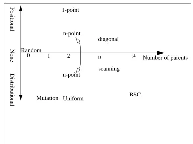
Representation of Space of Reproduction Operators 25 Block Conflict with Non-Adjacent Linkage 32
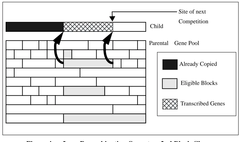
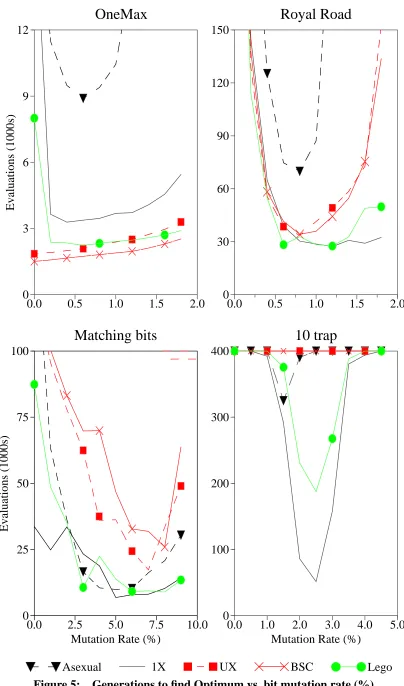
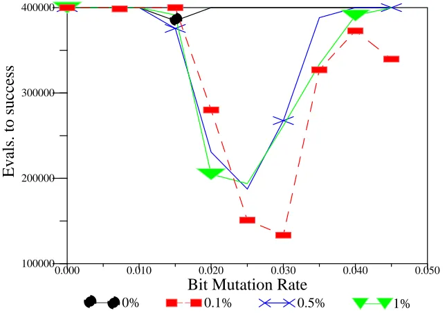
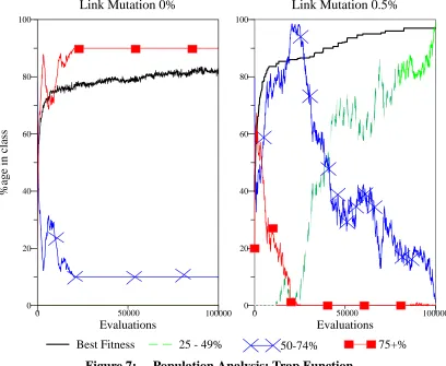
Lego Recombination Operator: 2nd Block Chosen 36 Generations to find Optimum vs. bit mutation rate (%) 39 Effect of varying link mutation rate: 10 trap function 40 Population Analysis: Trap Function 41
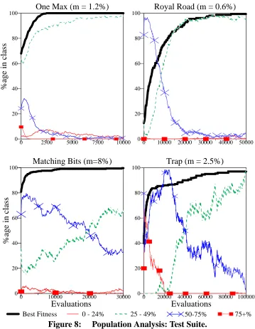
Population Analysis: Test Suite. 43
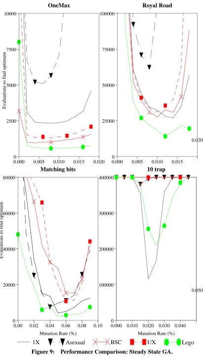
Performance Comparison: Steady State GA. 45
Performance Comparison SSGA vs. GGA, Lego Operator 47 Population Analysis: SSGA 0.5% Link Mutation 48
Population Analysis: SSGA 0.1% Link Mutation 49
Population Analysis: Size 500, Fifo deletion, Link Mutation 0.1% 50 Linkage Evolution with Adjacent Epistasis: N = 16 54
Linkage Evolution with Adjacent Epistasis: N = 32 55
Linkage Evolution with Varying Random Epistasis: N = 16 57 Linkage Evolution: Random vs. Adjacent Epistasis 59
Mean Number of Parents per Offspring 60 Replacement Policy Comparison 68
Evolved Mutation Rates with Different Recombination Operators 70 Comparison of Different Values ofλ 73
Adaptive vs. Standard GAs: Conditional Replacement 76 Adaptive vs. Standard GAs: Elitist Replacement 78 Adaptive vs. Hybrid GA’s: Conditional Replacement 80 Comparison of Adaptive GA with Hybrid GAs: Elitist 82 Evolved Mutation Rates vs. Number of Evaluations,λ = 5 84 Evolution of Mutation Rate: Varying Lambda, K = 4 86 Survival Rates under Mutation 87
Evolved Behaviour: Adapt1 Algorithm 95 Evolved Behaviour AdaptM Algorithm 96
Generations to find optimum at optimal mutation rate 38 Recombination Comparison: Mean of Best Values Found 62 Recombination Policy Comparison 69
Mutation Encoding Comparisons 71
Effect of Changing Maximum Decoded Mutation Rate 71 Final Fitness Comparison: Varyingλ 74
Best Value Found: Conditional Replacement, Standard GAs 75 Best Value Found: Elitist Replacement, Standard GAs 77 Best Value Found: Conditional Replacement, Hybrid GAs 79 Best Value Found: Elitist Replacement, Hybrid GAs 81 Best Algorithm for each Problem Class 83
Self-Adaptation in Evolutionary Algorithms
Introduction
Evolutionary Algorithms are search algorithms based on the Darwinian metaphor of “Natural Selection”. Typically these algorithms maintain a finite memory, or “population” of individual solutions (points on the search landscape), each of which has a scalar value, or “fitness” attached to it, which in some way reflects the quality of the solution. The search proceeds via the iterative generation, evaluation and possible incorporation of new individuals based on the current population.
A number of classes of Evolutionary Algorithms can (broadly speaking) be distinguished by the nature of the alphabet used to represent the search space and the specialisation of the various operators used, e.g. Genetic Algorithms ([Holland, 1975]: binary or finite discrete representations), Evolution Strategies ([Rechenberg, 1973, Schwefel, 1981]: real numbers) Evolutionary Programming ([Fogel et al., 1966]: real numbers), and Genetic Programming ([Cramer, 1985, Koza, 1989]: tree based representation of computer programs). This thesis is primarily concerned with Genetic Algorithms (GAs) based on a binary problem representation, since these can be used to represent a wide range of problems (ultimately, any problem that can be represented in a computer).
Although not originally designed for function optimisation, Genetic Algorithms have been shown to demonstrate an impressive ability to locate optima in large, complex and noisy search spaces. One claim frequently made is that the GA is a robust algorithm, i.e. that is it is relatively insensitive to the presence of noise in the evaluation signal. However it is recognised that the performance is greatly affected by the choice of representation, size of population, selection method and genetic operators (i.e. the particular forms of recombination and mutation and the rate at which they are applied). It is easily shown that poor choices can lead to reduced performance, and there is a further complication in the fact that both empirical (e.g. [Fogarty, 1989]) and theoretical (e.g.[Back, 1992a]) studies have shown that the optimal choice is dependant not only on the nature of the landscape being searched but of the state of the search itself relative to that landscape.
In this thesis a number of mechanisms are proposed and investigated within which the parameters governing search are encoded with the individuals and are able to adapt subject to the same evolutionary pressures and mechanisms as the candidate solutions. This is known as Self Adaptation of the search strategies.
These mechanisms allow the problem and parameter spaces to be searched in parallel, and by the choice of a suitable representation the range of strategies accessible is extended beyond those available to “standard” genetic algorithms.
Using the metric of the best value found in a given number of evaluations, it is shown that these algorithms exhibit superior performance on a variety of problem types when compared to a range of “standard” GAs. Furthermore, analysis of the reproduction strategies which evolve in the adaptive algorithms shows that the behaviours displayed correspond well to what is known about the nature of the search landscapes. Finally methods are suggested for utilising this correspondence to obtain on-line estimates of the nature of an unknown landscape, and to apply them to facets such as population sizing.
Organisation
This thesis is organised as follows:
In Chapter One the basic genetic algorithm is introduced and the various operators described. A review of previous work on optimisation of control parameters is given, followed by a discussion of a number of schemes that have been proposed for adapting operators and parameters during the course of evolution. A framework is presented within which these adaptive algorithms can be classified.
Building on this, in Chapter Three a Self-Adaptive mechanism is introduced based on the principles developed. Performance comparisons against a range of widely used crossover operators are presented, and the effect of changing other search parameters is investigated.
In Chapter Four, Kauffman’s NK-family of search landscapes are introduced [Kauffman, 1993]. These are a set of tunable landscapes with well known statistical characteristics. An analysis is then given of the recombination strategies which evolve on different types of landscapes, in the light of their known properties. Results are also presented from performance comparisons with other recombination operators. Finally it is suggested that in addition to being effective in an optimisation setting, observations of the strategies evolving may be used to characterise the landscape being searched.
In Chapter Five the focus is turned to mutation, and the application of some ideas from Evolutionary Strategies to Steady State GAs is investigated. The effect of changing other search parameters and incorporating an element of local search is investigated and the performance compared with a variety of widely used and recommended fixed mutation rates. An analysis is made of the mutation rates evolved on different classes of landscapes, and with differing amounts of local search. Following this reasons are given for the empirically observed superior performance of the local search mechanism.
In Chapter Six two possible ways of merging the methods described above are considered. Both of these produce a single reproduction operator within which both the units of heredity (which determine recombination strategy) and the mutation rate(s) applied are allowed to evolve. Performance comparisons and a range of analysis tools are used to investigate the synergistic effects of co-evolving the recombination and mutation strategies.
Finally, in Chapter Seven, conclusions and a number of suggestions for future work are presented.
Some of the work contained in this thesis has previously been published elsewhere, specifically: parts of Chapter One have been published in [Smith and Fogarty, 1997a],
parts of Chapters Two and Three have been published in [Smith and Fogarty, 1995], parts of Chapter Four have been published as [Smith and Fogarty, 1996b],
parts of Chapter Five have been published as [Smith and Fogarty, 1996c] and parts of Chapter Six are based on work published as [Smith and Fogarty 1996a].
Acknowledgements
Chapter One
Operator and Parameter Adaptation in Genetic Algorithms
1. A Background to Genetic Algorithms
Genetic Algorithms [Holland, 1975] are a class of population based randomised search techniques which are increasingly widely used in a number of practical applications. Typically these algorithms maintain a number of potential solutions to the problem being tackled, which can be seen as a form of working memory - this is known as the population. Iteratively new points in the search space are generated for evaluation and are optionally incorporated into the population.
Attached to each point in the search space will be a unique fitness value, and so the space can usefully be envisaged as a “fitness landscape”. It is the population which provides the algorithm with a means of defining a non-uniform probability distribution function (p.d.f.) governing the generation of new points on the landscape. This p.d.f. reflects possible interactions between points in the population, arising from the “recombination” of partial solutions from two (or more) members of the population (parents). This contrasts with the globally uniform distribution of blind random search, or the locally uniform distribution used by many other stochastic algorithms such as simulated annealing and various hill-climbing algorithms.
The genetic search may be seen as the iterated application of two processes. Firstly Generating a new set of candidate points, the offspring. This is done probabalistically according to the p.d.f. defined by the action of the chosen reproductive operators (recombination and mutation) on the original population, the parents. Secondly Updating the population. This usually done by evaluating each new point, then applying a selection algorithm to the union of the offspring and the parents.
1.1. Some Definitions
The Genetic Algorithm can be formalised as:
(D1) where
P0= (a10,..., aµ0) ∈ Iµ Initial Population
I = {0,1}l Binary Problem Representation
δ0 ⊆ ℜ Initial Operator Parameter set
µ ∈ Ν Population Size
λ ∈ Ν Number of Offspring
l ∈ Ν Length of Representation
F : I → ℜ+ Evaluation Function G : Iµ →Iλ Generating function U : Iµ x Iλ →Iµ Updating function
For the purposes of this discussion it has been assumed that the aim is to maximise the evaluation function, which is restricted to returning positive values. Although the fitness function is usually seen as a “black box”, this restriction will always be possible by scaling etc.
A broad distinction can be drawn between the two types of reproductive operators, according to the number of individuals that are taken as input. In this thesis the term Mutation operators is used for those that act on a single individual, producing one individual as the outcome, and Recombination operators for those that act on more than one individual to produce a single offspring. Typically, recombination operators have used two parents, and the term “crossover” (derived from evolutionary biology) is often used as a synonym for two-parent recombination.
Since all recombination operators involve the interaction of one individual with one or more others, the general form of these functions is:
R : Iµ x δ → I Recombination Operator (D2)
where the individuals taking part are drawn from {1...µ} according to some probability distribution pr, as opposed to the general form:
M : I x δ → I Mutation Operator (D3)
Using O∈Iλ to denote the set of offspring, an iteration of the algorithm becomes:
Oit= M R (Pt,δt) ∀i∈ {1...λ} (D4)
Pt+1=U (Ot ∪Pt) (D5)
The “canonical GA” as proposed by Holland is referred to as a Generational GA (GGA). It uses a selection scheme in which all of the population from a given generation is replaced by its offspring, i.e.λ = µ , and U is defined by the p.d.f. pu (ait) where
(D6) Parents for the next round of recombination are chosen with a probability proportional to their relative fitness, R drawing individuals from {1...µ} with a probability distribution function prgiven by:
(D7)
Holland, and later DeJong also considered the effect of replacing a smaller proportion of the population in any given iteration (known as generations). At the opposite end of the spectrum to generational GAs lie “steady state” genetic algorithms (SSGAs) such as the GENITOR algorithm [Whitley and Kauth, 1988]. These replace only a single member of the population at any given time (λ = 1).
It can be shown that under the right conditions, the two algorithms display the same behaviour. In an empirical comparison [Syswerda, 1991] the two variants, were shown to exhibit near identical growth curves, provided that a suitable form of puwas used to define U for the SSGA. In this case random deletion was used i.e.
(D8)
These results are well supported by a theoretical analysis [DeJong and Sarma, 1992] using deterministic growth equations (in the absence of crossover and mutation).This showed that the principal difference is that algorithms displaying a low ratio ofλ:µ(SSGAs) display higher variance in their behaviour than those with higher ratios (e.g. 1 for GGAs). This variance decreases with larger populations, but was the basis behind early recommendations for generational algorithms (e.g. Holland’s original work and the empirical studies in [DeJong, 1975]) where small populations were used. It was also found that the use of strategies such as “delete-oldest” (a.k.a. FIFO) reduced the observed variance in behaviour whilst not affecting the theoretical performance.
However in practice, it is usual to employ techniques such as “delete-worst” in steady state algorithms. This can be seen as effectively increasing the selection pressure towards more highly fit individuals, and it has been argued that it is this factor rather than any other which accounts for differences in behaviour [Goldberg and Deb, 1991].
In fact since the algorithm is iterative, the two selection distributions are applied consecutively, and so they can be treated as a single operator U with a p.d.f. given by
ps(ait) = pr (ait) * pu (ait-1) (D9) pu( )ait 0 i P
t
∈
1 i∈Ot
=
pr( )ait
F at i ( )
F a tj( ) j=1
µ
∑
---=
pu( )ait
n–1 n
--- i∈Pt 1 i∈Ot
1.1. Building Blocks and the The Schema Theorem
Since Holland’s initial analysis, two related concepts have dominated much of the theoretical analysis and thinking about GAs. These are the concepts of Schemata and Building Blocks. A schema is simply a hyper-plane in the search space, and the common representation of these for binary alphabets uses a third symbol- # the “don’t care” symbol. Thus for a five-bit problem, the schema 11### is the hyperplane defined by having ones in its first two positions. All strings meeting this criterion are examples of this schema (in this case there are 23 = 8 of them). Holland’s initial work showed that the analysis of GA behaviour was far simpler if carried out in terms of schemata. He showed that a string of length l is an example of 2lschemata, although there will not in general be as many asµ* 2ldistinct schemata in a population of sizeµ. He was able to demonstrate the result that such a population will usefully process O(µ3) schemata. This result, known as Implicit Parallelism is widely quoted as being one of the main factors in the success of GAs.
Two features are used to describe schemata, the order (the number of positions in the schema which do not have the # sign) and the defining length (the distance between the outermost defined positions). Thus the schema H = 1##0#1#0 has order o(H) = 4 and defining length d(H) = 8.
For one point crossover, the schema may be disrupted if the crossover point falls between the ends, which happens with probability d(H) / (l -1). Similarly uniform random mutation will disrupt the schema with a probability proportional to the order of the schema.
The probability of a schema being selected will depend on the fitness of the individuals in which it appears. Using f(H) to represent the mean fitness of individuals which are examples of schema H, and fitness proportional selection as per (D7), the proportion m(H) of individuals representing schema H at subsequent time-steps will be given by:
m(H, T+1) = m(H,t) * probability of selection * (1 - probability of disruption).
In fact this should be an inequality, since examples of the schema may also be created by the genetic operators. Taking this into account and using the results above gives
(1) This is the Schema Theorem.
A related concept is the Building Block Hypothesis (see [Goldberg, 1989 pp 41-45] for a good description). Simply put, this is the idea that Genetic Algorithms work by discovering low order schemata of high fitness (building blocks) and combining them via recombination to form new potentially fit schemata of increasing higher orders. This process of recombining building blocks is frequently referred to as mixing.
1.2. Operator and Parameter Choice
The efficiency of the Genetic Algorithm can be seen to depend on two factors, namely the maintenance of a suitable working memory, and quality of the match between the p.d.f. generated and the landscape being searched. The first of these factors will depend on the choices of population size
µ, and selection algorithm U. The second will depend on the action of the reproductive operators (R and M) and the set of associated parametersδ, on the current population.
Naturally, a lot of work has been done on trying to find suitable choices of operators and their parameters which will work over a wide range of problem types. The first major study [DeJong, 1975] identified a suite of test functions and proposed a set of parameters which it was hoped would work well across a variety of problem types. However later studies using a “meta-ga” to learn suitable values [Grefenstette, 1986] or using exhaustive testing [Schaffer et al., 1989] arrived at different conclusions. Meanwhile theoretical analysis on optimal population sizes [Goldberg, 1985] started to formalise the (obvious?) point that the value ofµ on the basis of which decisions could be reliably made depends on the size of the search space.
The next few years of research saw a variety of new operators proposed, some of which (e.g. Uniform Crossover [Syswerda, 1989]) forced a reappraisal of the Schema Theory and led to the
m H t( , +1) m H t( , ) f H( ) f
--- 1 pc d H( ) l–1
---⋅
– – pm⋅o H( )
⋅ ⋅
focusing on two important concepts.
The first of these, Crossover Bias [Eshelman et al., 1989], refers to the differing ways in which the p.d.f.’s arising from various crossover operators maintain hyperplanes of high estimated fitness during recombination, as a function of their order and defining length. This is a function of the suitability of the p.d.f. induced by the recombination operator to the landscape induced by the problem encoding. These findings have been confirmed by more formal analysis on the relative merits of various recombination mechanisms [DeJong and Spears, 1990, 1992, Spears and DeJong, 1991].
The second concept was that of Safety Ratios [Schaffer and Eshelman, 1991] i.e. of the ratio of probability that a new point generated by the application of reproductive operators would be fitter than its parent(s) to the probability that it is worse. These ratios were shown empirically to be different for the various reproductive operators, and also to change over time. Again these reflect the match between the p.d.f.s induced by given operators on the current population to the fitness contours of the landscape.
This can be demonstrated by a thought experiment using the simplest case of the OneMax function:
(D10) In a random initial population, an average of half of the genes will have the non-optimal value, and so on average half of all mutations will be successful. However, as the search progresses, and the mean fitness of the population increases, the proportion of genes with the optimal value increases, and so the chance that a randomly distributed mutation will be beneficial is decreased. This was formalised in [Bäck, 1992a, 1993] where an exact form for the Safety Ratio was derived for a mutation probability p. This could not be solved analytically, but was optimised numerically and found to be well fitted by a curve of the form:
As can be seen, this is obviously time-dependant in the presence of any fitness-related selection pressure.
These considerations, when coupled with interactions with other Evolutionary Algorithm communities who were already using adaptive operators (e.g. the (1+1) [Rechenberg, 1973] and (µ λ) [Schwefel, 1977, 1981] Evolutionary Strategies), has led to an ever increasing interest in the possibilities of developing algorithms which are able to adapt one or more of their operators or parameters in order to match the p.d.f. induced by the algorithm to the fitness landscape.
In terms of the formalisation above, this equates to potentially allowing for time variance in the functions R,M and U, the parameter setδ, and the variables µ,and λ.It is also necessary to provide some set of update rules or functions to specify the form of the transitions Xt→Xt+1(where X is the facet of the algorithm being adapted).
As soon as adaptive capabilities are allowed, the size of the task faced by the algorithm is increased, since it is now not only traversing the problem space but also the space of all variants of the basic algorithm. This traversal may be constrained, and may take several forms, depending on the scope of change allowed and the nature of the learning algorithm. It may vary from the simple time-dependant decrease in the value of a single parameter according to some fixed rule (e.g [Fogarty, 1989]) to a complex path which potentially occupies any position in the hyper space defined by variations in R, M andδ, and which is wholly governed by self-adaptation and the updating process (e.g. [Smith and Fogarty, 1996a]).
If the exact nature of the search landscape is known, then it may be possible to follow the optimal trajectory through algorithmic space for a given problem. Unfortunately this will not generally be the case, and in practice it is necessary to provide some kind of learning mechanism to guide the trajectory. Inevitably there will be an overhead incurred in this learning, but the hope is that even allowing for this, the search will be more efficient than one maintaining a fixed set of operators and parameters.
f a( ) ai i=0
l
∑
=popt 1
2 f a( ( )–1)–l
In fact, the “No Free Lunch” theory [Wolpert and Macready,1995] tells us that averaged over all problem classes, all non-revisiting algorithms will display identical performance. Since for fixed operator/parameter sets there will be problems for which they are optimal, it follows that there must be other classes of problems for which the performance is very poor. The intention behind the use of adaptive operators and parameters within GAs is to create algorithms which display good “all-round” performance and are thus reliable for use as optimisers on new problems.
1.3. A Framework for Classifying Adaptation in Genetic Algorithms
The various methods proposed for incorporating adaptation into Genetic Algorithms, may be categorised according to three principles, namely What is being adapted (operators, parameters etc.), the Scope of the adaption (i.e. does it apply to all the population, individual members or just sub-components) and the Basis for change (e.g. externally imposed schedule, fuzzy logic etc.). In the following sections these principles are described in more depth, along with some examples of each type of adaptation.
1.3.1. What is being Adapted?
As has been described above, the genetic algorithm may be viewed as the iterated application of two processes: Generating new points in the landscape (via probabalistic application of recombination and/or mutation operators to the previous population), and Updating (via selection and resizing) to produce a new population based on the new set of points created and (possibly) the previous population.
The majority of the proposed variants of the simple genetic algorithm only act on a single operator, and furthermore it is true to say that most work has concentrated on the reproductive operators i.e. recombination and mutation. Whilst considerable effort has been expended on the question of what proportion of the population should be replaced at any given iteration, the function U, used to update the population, once chosen, tends to be static.
Much theoretical analysis of GA’s has focused on the twin goals of exploration of new regions of the search space and exploitation of previously learned good regions (or hyperplanes) of the search space. The two terms may be explained by considering how the p.d.f.s governing generation of new points change over algorithmic time, remembering that the p.d.f.s are governed jointly by the actions of the reproduction and selection operators. An explorative algorithm is one in which a relatively high probability is assigned to regions as yet unvisited by the algorithm, whereas an exploitative algorithm is one in which the p.d.f. represents rather accumulated information about relatively fitter regions and hyperplanes of the search space. Thus the p.d.f. of an explorative algorithm will change more rapidly than that of an exploitative one.
Broadly speaking most adaptive algorithms work with the settings of either a Generational GA (GGA) or a “Steady State” GA (SSGA) which represent the two extremes of i) generating an entirely new population (through multiple reproductive events) and ignoring the previous population in the selection process or ii) generating and replacing a small number (usually one) of individuals (via a single reproductive event) at each iteration.
If the reproductive operators which are applied produce offspring that are unlike their parents, then the updating mechanisms of GGAs and SSGAs may be seen as favouring exploration and exploitation respectively. (Note that the equivalence of the growth curves for SSGAs and GGAs described earlier on page 10 was only in the absence of crossover or mutation).
However the extent to which offspring differ from their parents is governed not simply by the type of operator applied, but by the probability of its application as opposed to simply reproducing the parents. Thus for a given population and reproductive operator, it is possible to tune the shape of the induced p.d.f. between the extremes of exploration and exploitation by altering the probability of applying the reproductive operator, regardless of the updating mechanism.
of the population which is replaced at each iteration, whilst using simple and efficient selection mechanisms. This allows the tuning of the updating mechanism to particular application characteristics e.g. the possibility of parallel evaluations etc.
A number of different strands of research can be distinguished on the basis of what the algorithms adapt, e.g. operator parameters, probabilities of application or definitions.
In some ways the simplest class are those algorithms which use a fixed set of operators and adapt the probability of application of those operators. Perhaps the two best known early examples of work of this type are the use of a time-dependant probability of mutation [Fogarty, 1989] and the use of varying probabilities of application for a few simple operators (uniform crossover, averaging crossover, mutation, “big creep” and “little creep”) depending on their performance over the last few generations [Davis, 1989]. Many later authors have proposed variants on this approach, using a number of different learning methods as will be seem later. A similar approach which changes the population updating mechanism by changing the selection pressure over time can be seen in the Grand Deluge Evolutionary Algorithm [Rudolph and Sprave, 1995].
An extension of this approach can be seen in algorithms which maintain distinct sub-populations, each using different sets of operators and parameters. A common approach is to use this approach with a “meta-ga” specifying the parameters for each sub-population- e.g. [Grefenstette, 1986, Kakuza et al., 1992, Friesleben and Hartfelder,1993] to name but three. Although the searches in different (sub)populations may utilise different operators, each can be considered to have the full set available, but with zero probability of applying most, hence these are grouped in the first category. A similar approach is taken to population sizing in [Hinterding et al., 1996]. All of this class of algorithms are defined by the set:
(D11) whereΓ:δ → δis the transition function such thatδt=Γ(δt-1). As has been described, the function
Γ will often take as parameters some “history” of relative performance, and the number of generations iterated. Note that hereλ andµare subsumed intoδ.
A second class of adaptive GA’s can be distinguished as changing the actual action of the operator(s) over time. An early example of this was the “Punctuated Crossover” mechanism [Schaffer and Morishima, 1987] which added extra bits to the representation to encode for crossover points. These were allowed to evolve over time to provide a 2 parent N-point recombination mechanism, where N was allowed to vary between zero and the length of the string. The Lego and related Apes mechanisms [Smith and Fogarty,1995, 1996a, 1996b] evolve the “units of heredity” which determine recombination and mutation mechanisms, through the use of genetic encoded “links” between loci on the representation.
In both of these cases, the form of the reproductive operators are constant but their expression is dependant the particular individuals to which they are applied. The definition of the population thus changes to Pt∈Iµ x Xµwhere the form of X will depend on the algorithm: for example in Schaffer and Morishima’s work X = {0,1}l-1with a 1 in position j denoting that crossover should take place after locus j. The information governing the crossover operator is genetically encoded, and subject to mutation and recombination along with the problem encoding. The transition function here is simply the genetic algorithm itself i.e.Γ = UMR.
Algorithms which encode their operators and/or parameters in the genotype and use transition functions of this form are generally referred to as Self-Adaptive.
Within the category of algorithms which change the form of their operators rather than simply the probability of application fall those algorithms which alter the mechanisms governing the updating of the working memory by continuously changing its size (e.g.[Smith R., 1993, Smith R. and Smuda, 1995, Arabas et al., 1994,). In the first two examples, the form of pu is determined by comparing pairs of individuals as matched during crossover. In the work of Arabas et al., each individual is given a “lifespan”, g, at the time of its creation, according to its relative fitness. The p.d.f. governing the creation of a new population thus changes according to the current state of the
population
i.e. P = (a1,..., aµ, g1,...gµ) and (D12)
This can be contrasted to the SSGA with FIFO deletion where the lifespan of every individual is µ evaluations.
An alternative approach is to alter the representation of the problem itself: this can be viewed as an attempt to make the landscape suit the p.d.f.s induced by the operators rather than vice-versa. Work on “Messy GA’s” ([Goldberg et al., 1989] and many subsequent publications) is based on finding appropriate linkages between genes, using a floating representation where the order of the variables is not fixed. Since the “cut and splice” recombination operator tends to keep together adjacent genes, this can be seen as moulding the landscape to suit the operators. Similarly the ARGOT strategy [Schaefer, 1987] adaptively resizes the representation according to global measures of the algorithm’s success in searching the landscape, and more recently work on co-evolving representations [Paredis, 1995] can be seen in this restructuring light, as can the Adaptive Penalty Functions of [Eiben and van der Hauw, 1997, Eiben et al. 1998].
1.3.2. What is the Scope of the Adaptation?
The terminology of [Angeline, 1995] defines three distinct levels at which adaptation can occur in evolutionary algorithms. Population-level adaptations make changes which affect the p.d.f. contribution from each member of the current population in the same way. Individual-level adaptations make changes which affect the p.d.f. contribution from each member of the population separately, but apply uniformly to each of the components of the individuals’ representation. At the finest level of granularity are Component-level adaptations, where the p.d.f. contributions from each component of each member may be changed individually.
Inevitably, the scope of the adaptation is partly determined by what facet of the algorithm is being adapted, and the nature of the transition function. Changes in population size [Smith, R. and Smuda 1995], or problem restructuring (e.g. [Schaefer, 1987, Eiben and van der Hauw, 1997, Eiben et al. 1998]) for example can only be population level adaptations. However changes in some operators can occur at any of the three levels (for example mutation rates in Evolutionary Strategies), and so the notion of Scope forms a useful way of distinguishing between algorithms.
The forms of Γ defined by different adaptive algorithms are all attempts to tune the p.d.f.s arising from the action of genetic operators on the population to the topography of the problem landscape. Earlier an algorithmic space was described encompassing any given variant of the GA, and adaptation was defined as a traversal of this algorithmic space. For population level changes the trajectory will be a single path, as all members of the algorithm’s population at any given time will share a common set of operators and parameters. For individual and component level adaptations, the path will be that of a cloud, as each member follows a slightly different course. This cloud is composed of a number of traces which may appear and disappear under the influence of selection. 1.3.2.1. Population-Level Adaptation.
Recall from above that Genetic Algorithms can be viewed as the iterated probabalistic application of a set of operators on a population, and that in most cases these operators are static - that is to say that their forms and parameters are fixed and apply uniformly to the whole population i.e. they are global. Population-level adaptation algorithms can be typified as using a fixed set of global operators, but allowing their parameters to vary over time. The most important parameter is of course the probability of application. The various “meta-ga” algorithms mentioned above, and the competing sub-populations of the breeder GA e.g. [Schlierkamp-Voosen and Mühlenbein, 1994] belong firmly to this level. In general algorithms using adaptation at the population level will take the form of (D11). They may differ in the set of operators used, but are principally distinguished by the transition functionΓ.
pu( )ait
0 gi≥t 1 gi<t
There are a number of theoretical results which provide support for this kind of approach, e.g. regarding the time-variance of the optimal mutation rate [Mühlenbein, 1992, Hesser and Manner, 1991] (see also the discussions Bäck’s results, and of Schaffer & Eshelman’s experimental results regarding the time dependencies of Safety Ratios for mutation and crossover, on page 12).
In [Fogarty, 1989] an externally defined form is used to reduce the mutation rate over time, in a similar fashion to the cooling schedules used in Simulated Annealing. However a more common approach is to adjust one or more parameters dynamically in accordance with the performance of the algorithm or some measured quantity of the population.
A well known, and popular approach (e.g. [Davis, 1989, Corne et al., 1994, Julstrom, 1995]) is to keep statistics on the performance of offspring generated by various reproductive operators relative to their parents. Periodically “successful” operators are rewarded by increasing their probability of application relative to less successful operators. This approach does require extra memory, since it is usually found necessary to maintain family trees of the operators which led to a given individual, in order to escape from credit allocation problems.
Other authors have proposed control strategies based on simpler measures. Eshelman and Schaffer use the convergence of the population to alter the thresholds governing incest prevention, and the time spent without improvement to govern the probability of restarting the GA using vigorous mutation [Eshelman and Schaffer, 1991]. This latter is similar to many strategies for tracking changing environments, where a drop in the performance of the best member of the current generation is used to trigger a higher rate of mutation e.g. [Cobb and Grefenstette, 1993].
In [Lee and Takagi, 1993] fuzzy rules are learned and used to control various parameters based on the relative performance of the best, worst and mean of the current population. This concept of observing the fitness distribution of the population and then altering parameters according to a set of rules is also used in [Lis, 1996] where the mutation rate is altered continuously in order to keep a fitness distribution metric - the “population dispersion rate” within a desired range.
A more complex approach, and one which at first appears to belong to the component level is that of [Sebag and Schoenauer, 1994] who maintain a library of “crossover masks” which they label as good or bad. Inductive learning is used to control application of crossover and the periodic updating of mask strengths. However the rules learnt to control crossover are applied uniformly and so this belongs firmly in the category of population-level adaptation.
Perhaps the most obvious method of achieving population-level adaptation is to dynamically adjust the size of the population itself by creating or removing members according to some global measurement. Two approaches have been recently reported. In [Smith R., 1993, Smith R.and Smuda, 1995] the size is adjusted according to estimated schema fitness variance, whereas in [Hinterding et al., 1996] three populations of different sizes are maintained, with periodic resizing according to their relative successes.
Finally many of the proposed methods of adapting representations mentioned above plainly fall into this category.
1.3.2.2. Individual Level Adaptation
An alternative approach to adaptation is centred on consideration of the individual members of the population rather than the ensemble as a whole. Thus as a simple example, a global level adaptation may vary the probability of mutation for the whole population, whereas an individual level algorithm might hold a separate mutation probability for each member of the population. Considering the p.d.f. governing generation as the sum of the contributions from each member, then population level changes affect the way in which the contributions are determined uniformly, whereas individual level adaptations affect the p.d.f. contributions for each member separately.
A frequently claimed justification for this approach is that it allows for the learning of different search strategies in different parts of the search space. This is based on the not unreasonable assumption that in general search space will not be homogeneous, and that different strategies will be better suited to different kinds of sub-landscape.
on the earth and trying to reach the highest point it can. If on a large flat region, it would be better employed using a wider search (more uniform p.d.f. i.e. exploration), whereas if dropped by chance in the Himalayas such a search might rapidly lead it out of the mountain range. In the latter case a more localised search (i.e. exploitation) would be far preferable.
Algorithms at this level have been proposed which fall into a number of different categories in terms of the basis and scope of adaptation.
Perhaps the most popular class are algorithms which encode some parameters for an operator into the individual and allow these to evolve, using the updating process itself as the basis for learning. An early example of this was the “Punctuated Crossover” mechanism of [Schaffer and Morishima, 1987]. This added a mask to the representation which was used to determine crossover points between two parents during recombination, and which was evolved along with the solutions (as described on page 14 above). The results reported were encouraging, but this may have been due to the high number of crossover points evolved (compared to the algorithm used for comparison). In [Levenick, 1995] a similar mechanism is investigated, but with the added bits coding for changes in crossover probability at those points rather than deterministic crossing.
A more complex version of these, which uses discrete automata to encode for the crossover probabilities at each locus, is discussed in [White and Oppacher, 1994]. In this algorithm the representation is extended to store the state of the automata at each locus i.e. ai= {0,1}lx {0,... n}l-1. Unlike the two algorithms just mentioned, the transition function Γ, which maps ait → ai’ t is not simply the combination of recombination and mutation acting on the genotypes prior to the action of selection. Rather a set of rules are applied based on the relative fitness of offspring and parents, which update the state of each automata.
An alternative method for controlling recombination strategies was used in [Spears, 1995] where a single bit was added to the genotype and used to decide whether two-point or uniform crossover would be used when an individual reproduced. Again self-adaptation was used for the transition. This control method differed from the above mechanisms in that they allow the form of the operator itself to change, whereas this algorithm effectively associates two operators with each individual and associates probabilities of 0 or 100% of application with each.
It is noticable that this was compared with a population level mechanism where the relative proportion of bits encoding for the two operators was used to make a global decision about operator probabilities. Although these two alternatives should provide the same ratio of usage of the two operators, the latter mechanism was found to work far less well, suggesting that there is indeed a merit in attaching reproductive strategies to particular individuals. Certainly the two methods can yield different p.d.f.s for the next generation of points.
Perhaps more common has been the adoption of the idea of self adaptive mutation rates from Evolutionary Strategies. The addition of extra bits to the genome to code for the mutation rate for that individual was first investigated for GGAs in [Bäck, 1992b]. It was found that the rates evolved were close to the theoretical optimum for a simple problem, providing that a sufficiently rigorous selection mechanism was used. The second level of adaptation in [Hinterding et al., 1996] uses a similar encoding to control the standard deviation of the Gaussian distributed random function used to mutate genes. In [Smith and Fogarty, 1996c] self adaptive mutation was translated into a Steady State algorithm, with the addition of a (λ,1) “inner GA”. This was found to be necessary to provide the selection pressure for self adaptation, but also provided a kind of local search.
However not all algorithms using adaptation at the individual level rely on endogenous control and self-adaptation. As with population level adaptations, a number of other algorithms can be used to control the behaviour of individuals.
p.d.f.s with the less fit members. Another approach based on relative local fitness in a structured population uses a pattern of rules to control the reproduction strategy (replication, crossover or mutation) based on metaphors of social behaviour [Mattfeld et al., 1994]. Similarly the Grand Deluge Evolutionary Algorithm of [Rudolph and Sprave, 1995] adapts the “acceptance” threshold governing the updating process separately for each point, based on relative local fitness over a period of time. Effectively all of these exogenously controlled algorithms take the form:
(D13) where there is now a vector of sets of parameters
Similarly measures of relative fitness and convergence are used to determine the “lifespan” given to a newly created individual in [Arabas et al., 1994]. This novel approach controls the contents and size of the working memory by assigning a fixed lifetime to each individual after which it is removed from the memory (see page 14). This is one of the very few algorithms reported providing dynamic population sizing, and the results reported suggest that this is a promising line of research. 1.3.2.3. Component-Level Adaptation
This is the finest level of granularity for adaptation: here algorithms allow different reproduction strategies for different parts of the problem representation. Again these ideas originate from Evolutionary Strategies research, which has progressed over the years from a single parameter controlling the mutation step size for the population, through individual step-sizes for each member, to having a separate mutation step size encoded for each component being optimised.
This can be considered as a means of allowing the focus of search to be directed, and the principal advantage is that it allows for a much finer degree of tuning of the p.d.f. contribution associated with each individual. All of the work done at this level has used self-adaptation as the method of learning parameters.
This approach was tried in the self-adaptive mutation mechanism of [Bäck, 1992b] and compared with individual level adaptation. Essentially a real-valued mutation rate was added for each locus i.e. ai = {0,1}l x ℜl. The results suggested that in certain circumstances the results were advantageous, but that on other landscapes the learning overheads associated with all the extra mutation parameters slowed the search down. The conclusions seemed to be that such a mechanism could be very effective if the components were properly defined i.e. the level of granularity was chosen suitably.
An attempt to solve some of these problems can be seen in the Lego mechanisms [Smith and Fogarty, 1995, 1996b]. These are somewhat similar to the “Punctuated Crossover” algorithms of Schaffer and Morishima in adding extra bits to the representation to determine whether two adjacent genes may be broken by crossover. However the emphasis is different, in concentrating on finding blocks of co-evolved linked genes. The recombination mechanism also differs in that blocks of genes may be chosen from the whole population (rather than just two parents) when a new individual is formed. This evolution of linkage has to be seen therefore as an adaptation of recombination strategy at the component level, since individuals have no meaning in the context of parents other than as contributing to a “genepool” from which new individuals are assembled. This emphasis on evolving successful components rather than individuals was taken further in the Apes algorithm [Smith and Fogarty, 1996a]. This included component level adaptation of mutation rates by attaching a mutation rate to each block, which is also self-adapted.
1.3.3. What is the Basis for Adaptation?
The final distinction between classes of adaptive genetic algorithms is perhaps the most important, namely the basis on which adaptation is carried out. This in turn hinges on two factors, firstly the evidence upon which adaptation is carried out, and secondly the rules or algorithm which define how changes are effected. In terms of our notation this second factor is the definition of the transition functionΓ, and the evidence translates to the choice of parameters or inputs for that function.
GA = (P0, ,δ0 l,F G U, , ,Γ)
The first distinction between kinds of adaptive algorithms is drawn on the basis of the evidence that they consider.
In one camp are all those algorithms which take as their evidence differences in the relative performance of strategies. These include Self-Adaptive and meta-GAs. Those algorithms which adjust operator probabilities based on records of performance, such as those of [Davis 1989, Corne et al. 1994, Julstrom 1995] fall into this category as their probabalistic nature allows the concurrent testing of multiple strategies (the difference being that they use predefined rules to adjust the strategies). Also into this category fall those algorithms which draw conclusions based on observations of strategy performance such as Sebag and Schoenauer’s Inductively Learned Crossover Masks, and White and Oppacher’s Automata Controlled Crossover.
Into the other camp fall those algorithms which adapt strategies based on empirical evidence which is not directly related to the strategy followed. This might be convergence statistics (in terms of the population fitness, or the allele distribution), observed relative schema fitnesses etc. Although some use simple rules e.g. previously learned Fuzzy Rule-Sets [Lee and Takagi, 1993] or predefined schedules [Fogarty, 1989], most base the derived trajectory on an attempt to fulfil some criterion or maintain a population statistic. Examples of this latter are the “Population Dispersal” metric of [Lis, 1996], and “Schema Fitness Variance” [Smith, R. and Smuda, 1995].
Consideration of the nature of the transition function itself suggests another important distinction that can be drawn between two types of algorithm. These have been labelled as “Uncoupled vs. Tightly Coupled” [Spears, 1995], or “Empirical vs. Absolute” update rules [Angeline 1995]. Essentially in the first type of algorithm, the transition function Γ is externally defined -previously referred to as exogenous algorithms. In the second type (endogenous algorithms) the operator parameters (and possible definitions) are encoded within individuals, andΓis itself defined by the genetic operators U, M and R, i.e.the GA itself is used to determine the trajectory. This latter approach is more commonly known as Self-Adaptation.
To clarify this point, in all algorithms a set of evidence is considered, on the basis of which the trajectory of the algorithm is decided. If the evidence is not relative strategy performance, then the control mechanism is necessarily uncoupled from the generation-updating mechanisms of the evolutionary algorithm itself. If the evidence is relative strategy performance, then the control mechanism may be externally provided (as in, for example, Davis’ work) or may be a function of the genetic operators of the algorithm itself i.e. Self Adaption.
In most uncoupled adaptive algorithms the evidence takes the form of statistics about the performance of the algorithm, such as the fitness distribution of the population, “family trees”, or simply the amount of evolutionary time elapsed. The important factor is that the mechanism used to generate the new strategies based on this evidence is externally provided in the form of a learning algorithm or a set of fixed rules.
A number of Self-Adaptive algorithms have been described above, and their reported success is perhaps not surprising in the light of the considerable research into these topics in the fields of Evolution Strategies and Evolutionary Programming. The rationale is essentially two-fold, firstly that if strategies are forced to compete through selection, then what better proof of the value of a strategy than its continued existence in the population. Secondly, and perhaps less tritely, the algorithmic space being searched has an unknown topography, but is certainly extremely large, very complex and highly epistatic, since there is a high degree of dependency between operators. Evolutionary Algorithms have repeatedly been shown to be good at searching such spaces...
operators and parameters will also be different.
1.4. Discussion
The framework proposed above categorises algorithms according to three principles. The first two of these are what features of the algorithm are susceptible to adaptation, and the granularity at which this is done. Separate from these, a further important distinction was drawn according to the basis for change. This took two forms, namely the type of evidence used as input to the strategy-deciding algorithm, and that algorithm itself.
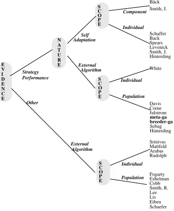
There are a number of possible ways of representing this categorisation, in Figure 1, a simplified taxonomic tree is shown to illustrate the main branches of Adaptive Genetic Algorithms (algorithms are referred to by their first authors).
The first branch of the tree is evidence for change (or more formally the inputs to the transition function). If this is the relative performance of different strategies then there is a further subdivision according to whether the transition function is tightly coupled (Self Adaptation) or uncoupled. If the input to the transition function is some feedback other than relative strategy performance, then the nature of the transition function is necessarily uncoupled from the evolutionary algorithm, so the second branch point does not apply. Below all these branches are leaves corresponding to the scope of the adaptation.
The nature of the field, and the absence of a standard test suite of problems make it impossible to compare algorithms on the basis of reported results and declare a universal winner. Indeed the very considerations that drive research into adaptive algorithms make such statements meaningless. It is however possible to draw a few conclusions.
Firstly, those algorithms based on observing the relative performance of different strategies appear to be most effective. This seems to follow naturally from the fact that GA theory is currently not sufficiently advanced either to permit the specification of suitable goals in terms of other metrics, or (more importantly) how to achieve them. It is ironic that perhaps the most widely quoted paper on adaptive strategies, the externally defined time-decreasing mutation rate of [Fogarty, 1989] is also one of the most widely misquoted works in the field, since this was concerned specifically with initially converged populations.
Secondly, there appears to be a distinct need for the maintenance of sufficient diversity with the population(s). It is the experience of several authors working with adaptive recombination mechanisms that convergence makes the relative assessment of different strategies impossible. Variety within the population is vital as the driving force of selective pressure in all Evolutionary Algorithms, and will be doubly so in Self-Adaptive algorithms. This is less of a problem for algorithms manipulating mutation rates as mutation is generally a force for increased diversity.
Thirdly, there are powerful arguments and empirical results for pitching the adaptation at an appropriate level. The success of individual level adaptive reproduction schemes appears convincing, and there is promise in the various methods proposed for identifying suitable components via linkage analysis which would allow adaptation at an appropriate level. However as Angeline points out, and Hinterding demonstrates, there is scope for adaptation to occur at a variety of levels with the GA
Chapter Two
Recombination and Gene Linkage
2. Introduction
Having previously discussed the rationale behind adaptive genetic algorithms, and provided a basis for the choice of self-adaption as the preferred method, this chapter concentrates on the recombination operator. It is this operator which principally distinguishes genetic algorithms from other algorithms, as it provides a means by which members of the population can interact with each other in defining the p.d.f. which governs the generation of new points in the search space.
2.1. The Importance of Recombination
Since Holland's original formulation of the GA there has been considerable discussion of, and research into, the merits of crossover as a search mechanism. Much of this work has been concentrated on contrasting the behaviour of algorithms employing recombination as one of the reproductive operators as opposed to those using only mutation-based operators. Into this second class fall algorithms such as Evolutionary Strategies (either (1+1)[Rechenberg, 1973] or (1,λ) [Schwefel, 1977]), Evolutionary Programming (Fogel et al. 1966), various Iterated Hillclimbing algorithms and other neighbourhood search mechanisms such as Simulated Annealing [Kirkpatrick et al.,1983].
The conditions have been studied in which sub-populations using crossover would “invade” populations using mutation alone by the use of a gene for crossover [Schaffer and Eshelman, 1991]. It was found that providing there was a small amount of mutation present then crossover would always take over the population. This was not always beneficial to the search, depending on the amount and “locality” of epistasis in the problem encoding.
They also confirmed empirically that the safety ratio of mutation decreased as the search continued, whereas the safety ratio of crossover (especially for the more disruptive uniform crossover) increased as the search progressed. For both algorithms the ratio was never above unity, i.e. offspring are more likely to be worse than better when compared to their parents.
Some reasons why mutation is decreasingly likely to produce offspring which are fitter than their parents were discussed earlier (see page 12). The probability that crossover will display an increasing safety ratio on a given problem representation depends on a number of factors. Although the state of GA theory is not sufficiently advanced to be prescriptive, two closely related factors which have been widely recognised and investigated are:
1. Crossover is much less effective than mutation at resisting the tendency of selection pressure towards population convergence - once all of the population has converged to the same allele value at a locus, crossover is unable to reintroduce the lost allele value[s], (unlike mutation). As a result of this, as the population converges and identical parents are paired with increasing frequency, crossover has less and less effect, sending the safety ratio towards unity. This was demonstrated in experiments using the adaptive “Punctuated Crossover” mechanism [Schaffer and Morishima, 1987] which allowed a traditional G.A. to learn binary decisions about effective crossover points at different stages of the search. It was found that as the search continued the number of encoded crossover points increased rapidly, although the number of productive crossover operations did not.
2. Until the population is almost entirely converged, crossover has a greater ability to construct higher order schemata from good lower order ones (the Building Block hypothesis). This ability is modelled theoretically in [Spears, 1992] where it is shown that crossover has a higher potential than mutation. The nature (in terms of order and defining length) of lower order schema that will be combined depends on the form of the crossover operator (this is discussed further in section 2.2), and so the quality of the higher order building blocks constructed will depend in part on a suitable match between the epistasis patterns in the representation and the operator.
high probability, then the Safety Ratio is likely to rise initially as these schema fitness estimates improve.
As the size of the building blocks increases over time there is a secondary effect that population convergence biasses the sampling which can have deleterious effects. However as noted, (and unlike mutation) the probability of constructing new high order hyperplanes depends on the degree of convergence of the population. Therefore whether the combination of relatively fit low order hyperplanes is beneficial or not, the effect on the Safety Ratio will diminish over time as the population converges.
Although Safety Ratios are a useful tool for understanding the differences between operators, they can also be misleading as they consider relative rather than absolute differences in fitness between offspring and parents. As an example on their “trap” function, Schaffer and Eshelman found that the ratio diminished over time for mutation and increased over time for Uniform Crossover, but the former had a far better mean best performance in terms of discovering optima.
The Royal Road landscapes [Mitchell et al., 1992, Forrest and Mitchell, 1992] were created with building blocks specifically designed to suit the constructive powers of crossover. Mitchell et al. compared results from algorithms using both crossover and mutation with those from iterated hillclimbing techniques. It was found that contrary to the authors' expectations, Random Mutation Hill Climbing outperformed algorithms using crossover on these “Royal Road” functions. Analysis showed that this was due to the tendency of crossover based algorithms (especially those using a low number of crossover points) to suffer from “genetic hitch-hiking” whereby the discovery of a particularly fit schema can lead to a catastrophic loss of diversity in other positions.
These issues have in fact been studied for many decades prior to the invention of genetic algorithms, or even modern computers. The origins of sexual recombination, and what benefits it confers, have long been studied by Evolutionary Biologists (see [Maynard-Smith, and Szathmary, 1995 chapter 9] for a good overview).
From the point of view of the “selfish gene” [Dawkins, 1976], it would initially appear that “parthenogenesis” (asexual reproduction) would appear to confer an advantage, since all of an organism’s genes are guaranteed (saving mutation) to survive into the next generation. It might be expected that a gene for parthenogenesis that arose by mutation in a sexually reproducing population would soon dominate. However, when a finite population is considered, the effects of Muller’s Ratchet [Muller, 1964] come into play. Simply stated, this is the effect that deleterious mutations will tend to accumulate in a population of fixed size. In practice this tendency is counteracted by selection, so that an equilibrium is reached. The point (i.e. the mean population fitness) at which this occurs is a function of the selection pressure and the mutation rate. By contrast, if recombination is allowed, then Muller’s ratchet can be avoided, and this has led to one view of the evolution of recombination as a repair mechanism - “It is now widely accepted that the genes responsible for recombination evolved in the first place because of their role in DNA repair” [Maynard-Smith, 1978, p36].
A second strand of reasoning used by biologists is similar to the Building Block hypothesis, and shows that in changing environments populations using recombination are able to accumulate and combine successful mutations faster than those without [Fisher, 1930]- this is sometimes known as “hybrid vigour”.
2.2. Recombination Biases
Considerable effort has been put into deriving expressions which describe the amount and type of schema disruption caused by various crossover operators and how this is expected to affect the discovery and exploitation of “good” building blocks. This has been explored in terms of positional and distributional biases, experimentally [Eshelman et al., 1989, Eshelman and Schaffer, 1994] and theoretically [Booker, 1992, Spears and DeJong, 1990, 1991].
falling between the ends of a schema H of order o will be directly proportional to d(H) according to d(H) / (l-1) as was seen earlier (page 11). In fact the probability of disrupting a schema is purely a function of d(H), and since all genes between the end of the representation and the crossover point are transmitted together, is independent of the value of o(H).
Distributional Bias is demonstrated by operators in which the probability of transmitting a schema is a function of its order. For example, Syswerda defines Uniform Crossover [Syswerda, 1989] as picking a random binary mask of length l, then taking the allele in the ith locus from the first parent if the corresponding value in the mask is 0, and from the second if it is 1. Since each bit in the mask is set independently, the probability of picking all o genes from a schema in the first parent is purely a function of the value of o and is independent of d(H): p(survival) = po(H), where p = 0.5. This can be generalised by considering masks which have a probability p (0 < p < 1.0) of having the value 0 in any locus, and so the amount of bias exhibited can be tuned by changing p.
Positional bias, the tendency to keep together genes in nearby loci, is responsible for the phenomenon of genetic hitch-hiking, whereby the genes in loci adjacent to or “inside” highly fit schemata tend to be transmitted by recombination along with them. This assigns to the hitch-hiking schemata an artificially high mean fitness since they will tend to be evaluated in the context of highly fit individuals. This is known as “spurious correlation” and can lead to a loss of diversity, and premature convergence to a sub-optimal solution, as the proportions of the hitch-hiking schema increase according to (1).
2.3. Multi-Parent and Co-evolutionary Approaches
Recently the investigation of multi-parent crossover mechanisms, such as Bit Simulated Crossover (BSC) [Syswerda, 1993], has led to more discussion on the role of pair-wise mating and the conditions under which it will have an advantage over population based reproduction. Empirical comparisons [Eshelman and Schaffer,1993] showed that for carefully designed “trap” functions pair-wise mating will outperform BSC. This was attributed to the high amount of mixing occurring in the BSC algorithm, compared to the delayed commitment shown by the pair-wise operators which enables the testing of complementary middle order building blocks. However it was concluded that “the unique niche for pair-wise mating is much smaller than most GA researchers believe, and that the niche for 2X (sic) is even smaller”
Work on multi-parent recombination techniques (with fixed numbers of parents) [Eiben et al.,1994, 1995] showed that for many standard test bed functions n-parental inheritance (with n greater than 2 but less than the size of the population) can be advantageous, although they identified problems with epistasis and multi-modal problems. Two of the operators they introduced for non-order based problems are “scanning crossover” and “diagonal crossover”. The former is similar to BSC in performing a new selection process from the pool of n potential parents at each locus, thus effectively co-evolving each position. In the absence of any selective pressure pr(this form is known as “uniform scanning”) this will introduce a distributional bias whose strength will depend on the number of parents in the pool (Eiben et al. refer to this number as the “arity” of the operator). Diagonal crossover is a (n-1)-point generalisation of traditional one-point crossover, where sections are read from the n parents successively. This will exhibit positional bias to a degree dependant on the arity.
The idea of co-evolving separate populations of sub-components was used in [Potter and DeJong, 1994] as an approach to function optimisation, with similar findings that the efficiency of the approach is lessened as the amount of epistasis increases, but that if the problem decomposition is suitable then improvements over the “standard” operators are attainable. However the system reported relies on user-specified problem decomposition, and each of the sub-species is optimised sequentially. This leads to questions as to which of the candidates fro