Flow prediction in brain aneurysms using OpenFOAM

(1)

Flow prediction in brain aneurysms using OpenFOAM

M. de Groot

(2)

(3)

Abstract

Methods to detect aneurysms in the brain have existed for some decades. A relatively new method, 3D rotational angiography (3DRA), has received a lot of attention in the last decade, because with it additional smaller aneurysms can be detected more easily in comparison to more conventional methods. The voxel data of 3DRA allows for reconstruction of the blood vessel geometry with relative ease, which makes it of particular interest in the study of computational fluid dynamics (CFD). Predictions made based on a CFD analysis are believed to become more and more important and may have consequences for the type of treatment a particular patient receives.

The immersed boundary (IB) method is one of many CFD methods available to perform nu-merical simulations. The strength of the IB method is that no complex or time consuming grid generation is required. Instead, it uses a Cartesian grid in which the geometry is immersed, and is only concerned with determining whether a grid cell is part of the geometry or not. Its simplicity makes the IB method an excellent combination with 3DRA. A disadvantage of the IB method is that often only a small portion of the grid cells is part of the geometry, especially for complex geometries, making it a rather expensive method in terms of computation time. In this thesis an effort is made to utilise the simplicity of the IB method to perform numerical simulations of blood flow in the human brain without having to rely on grid cells which are not part of the geometry. Simulations are performed with an open source CFD software package, called OpenFOAM, which requires a number of input files to specify the grid. The challenge is to find an efficient way to remove the cells which are not part of the geometry from the grid and to generate the input files accordingly.

(4)

(5)

Introduction

A description is given of how the equations which govern fluid flow are solved using the open source CFD software package OpenFOAM and how these computations can be done in parallel. First, the governing equations for fluid flow, the Navier-Stokes equations, are presented. Subse-quently, an explanation of the adopted numerical method in OpenFOAM is given. Finally, it is shown how parallel computation can be done in OpenFOAM.

Starting from a masking function, the key element in a volume-penalising immersed boundary method which represents the geometry by taking either values ’0’ or ’1’ depending on whether a cell is in the fluid part or in the solid part of the domain, a geometry is constructed in OpenFOAM which only consists of cells which are in the fluid part of the domain. The method is validated with Poiseuille flow through a cylindrical pipe. Several measures are defined which are used to check how sensitive the solution is to refinement of the grid. Finally, the computational domain of the cylindrical pipe is decomposed in different ways, which is then used to see how the speedup of the computation is affected by different decompositions.

Another convergence study is done for Poiseuille flow through curved pipes, which have a sinusoidal shape. For these type of flows no analytical solution exists. Therefore, the previously mentioned measures are slightly altered such that they can still be used to investigate how sensi-tive the solution is to grid refinement. Finally, a realistic geometry is taken under consideration. A comparison is done between Poiseuille flow and physiologically relevant flow. Significant differ-ences in flow behavior are observed and an attempt is made to test the sensitivity of the solution to refinement of the grid.

The thesis is organised as follows. In Chapter 2 the adopted numerical method in OpenFOAM is described, followed by an explanation of parallel computation in OpenFOAM. The construction of geometries from the masking function of a volume-penalising immersed boundary method is explained in Chapter 3, after which it is validated with Poiseuille flow through a cylindrical pipe. The speedup of computation is tested by decomposing the cylindrical pipe in several ways. In Chapter 4 also Poiseuille flow through curved pipes is considered, which then bridges the gap to Poiseuille flow through realistic geometries. The chapter is concluded with physiologically relevant flow through through a realistic geometry.

(8)

(9)

Chapter 2

Computational model

This chapter is devoted to the Navier-Stokes equations and their respresentation in OpenFOAM. The process of solving these equations in OpenFOAM is explained in detail through an example of an initial-boundary value problem for the diffusion equation.

2.1 Navier-Stokes equations

The motion of incompressible Newtonian fluids in Cartesian coordinates is governed by the continuity equation

∇ ·u= 0, (2.1)

which reflects the conservation of mass, and the equations describing conservation of momentum, which are known as the Navier-Stokes equations,

∂tu+∇ ·(uuT) =−∇P+∇ ·(ν∇u), (2.2)

with fluid velocityu(x, t), kinematic pressureP(x, t) and kinematic viscosityν.

Boundary conditions are u = 0 at solid boundaries and the domain is periodic in the x

-direction. Because pressure is relative in a closed incompressible system, the absolute value of

pressure is not important. Hence, the initial conditions for velocity are chosen asu=0and for

pressure asP = 0.

The volumetric flow rateQis fixed and a pressure drop is imposed to force the flow. To be

able to impose periodic boundary conditions on the pressure and to have a pressure drop, the pressure term has to be modified. This can be achieved by splitting the pressure gradient in a gradient of the periodic component of the pressure and a term which gives the desired pressure drop as follows

∇P(x, t) =∇p˜(x, t) +∇p(t). (2.3)

2.2 Numerical method and OpenFOAM

Consider the diffusion equation

∂tT− ∇ ·(DT∇T) = 0, (2.4)

with temperature T = T(x, t) and diffusion coefficient DT. This equation is represented in

OpenFOAM as

(10)

Chapter 2. Computational model 4

s o l v e (

fvm :: ddt ( T ) - fvm :: l a p l a c i a n ( DT , T ) );

which is very intuitive; it looks similar to (2.4). Terms starting withfvm::are implicit terms and

explicit terms start withfvc::.

Now consider the following one-dimensional initial-boundary value problem for the diffusion equation     

∂tT −∂x(DT∂xT) = 0 for 0< x < Lxandt >0,

T(x,0) =f(x), for 0< x < Lx,

T(0, t) =T(Lx, t) = 0, fort >0,

(2.5)

with constant diffusion coefficientDT.

By introducing the scaling

ˆ

x= x

X, tˆ= t τ,

ˆ

T = T

T, fˆ=

f

T, (2.6)

the problem can be transformed to the dimensionless initial-boundary value problem



 

 

∂tT−∂x(1∂xT) = 0 for 0< x <1 andt >0,

T(x,0) =f(x), for 0< x <1,

T(0, t) =T(1, t) = 0, fort >0,

(2.7)

where hats have been dropped.

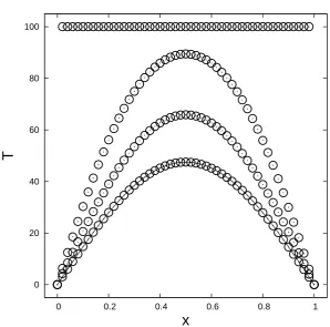
In the following an example case in OpenFOAM will be worked out. The problem given above will be represented as a rectangular copper rod with 1 meter length with initial temperature

distribution f(x) = T0 = 100. OpenFOAM uses physical quantities to be able to perform

dimension checks in its calculations. An analytical solution from the dimensionless problem will be used later, after rescaling, to validate the numerical solution which is obtained with OpenFOAM.

Setting up a case consists of several steps:

• Construct the mesh in the OpenFOAM mesh format, polyMesh

• Set parameters related to the problem

• Define initial and boundary conditions for each of the variables

• Select numerical schemes for each of the terms in the differential equation

• Specify solving algorithm and stop criteria per variable

• Set time control parameters and output settings

For a simple case like this, the geometry can easily be constructed using the mesh generation utility blockMesh, which is supplied with OpenFOAM. Geometries in OpenFOAM are always three-dimensional, even for a one-dimensional problem like in this example. In a dictionary file called blockMeshDict, which is located in the ‘constant/polyMesh’ directory for a given case, settings denoted by keywords are specified which are used by blockMesh to generate mesh files according to the polyMesh format. Below is the relevant part of the blockMeshDict file for this

(11)

5 2.2. Numerical method and OpenFOAM

this case. With the keyword vertices the (unscaled) coordinates of the corners of the rod are

defined. The position of each coordinate in the list determines its label (0,1, . . .). On the line

labeled with the keywordblocksthree characteristics of the mesh are defined. First the geometry

is defined by giving the coordinate labels in a specific order, followed by the number of cells in each direction and finally the expansion ratios of the cells in each direction. These expansion ratios are defined as the ratio between the width of the last cell to the width of the first cell.

The boundaries are specified in the last part denoted by the keywordboundary.

c o n v e r t T o M e t e r s 1; v e r t i c e s

(

(0 0 0) (1 0 0) (1 0.1 0) (0 0.1 0) (0 0 0 . 1 ) (1 0 0 . 1 ) (1 0.1 0 . 1 ) (0 0.1 0. l ) );

b l o c k s (

hex (0 1 2 3 4 5 6 7) ( 1 0 0 0 1 1) s i m p l e G r a d i n g (1 1 1) );

b o u n d a r y (

p a t c h 1 {

t y p e p a t c h ; f a c e s (

(0 4 7 3) );

} p a t c h 2 {

t y p e p a t c h ; f a c e s (

(1 2 6 5) );

} p a t c h 3 {

t y p e e m p t y ; f a c e s (

(0 3 2 1) (4 5 6 7) (0 1 5 4) (2 3 7 6) );

} );

The keywords patch1 andpatch2 correspond to the boundaries at x= 0 and x= 1 respectively

(12)

which causes OpenFOAM to interpret the problem as a one-dimensional problem. After running blockMesh a number of files will be generated in the ‘constant/polyMesh’ directory. The file

points containing coordinates of vertices of the cells, the file faces defining faces of the cells,

the files owner and neighbour defining connectivity of the mesh and the file boundary giving

information about boundaries of the mesh.

The only parameter in this problem is the diffusion coefficient, which for copper is DT =

1.11·10−4, and it is specified in the dictionary file transportProperties, which can be found in

the ‘constant’ directory, as follows

DT DT [ 0 2 -1 0 0 0 0 ] 1 . 1 1 e - 0 4 ;

The seven scalars delimited by square brackets correspond to the powers of the SI base units,

which are defining the units of measurement (m2/s) for the specified quantity.

Initial and boundary conditions are specified in the fileT in the ‘0’ directory. For this example

the file is shown below. First, the dimensions of the variableT (K) are defined. Of course, for

this particular example one would rather think in degrees Celcius (◦C), but a transformation

from degrees Celcius to Kelvin does not change the nature of the problem. On the next line,

denoted byinternalField, the initial value (100) is assigned to all cells. More specificly, the values

are defined at the centres of the cells. The last part, with the keywordboundaryField, specifies

boundary conditions;T = 0 at x= 0 andx= 1, and anemptyboundary on the remaining sides

of the rod, as before.

d i m e n s i o n s [0 0 0 1 0 0 0]; i n t e r n a l F i e l d u n i f o r m 1 0 0 ; b o u n d a r y F i e l d

{

p a t c h 1 {

t y p e f i x e d V a l u e ; v a l u e u n i f o r m 0; }

p a t c h 2 {

t y p e f i x e d V a l u e ; v a l u e u n i f o r m 0; }

p a t c h 3 {

t y p e e m p t y ; }

}

Integration of (2.4) over a control volumeV with boundary S gives

∂t

Z

V

T dV − Z

S

(DT∇T)·dS= 0. (2.8)

IfTi is defined as

T_in:=Ti(t=tn) =

1

Vi

Z

Vi

T(x, t=tn)dV , (2.9)

then (2.8) becomes

(∂tTi)n+1−

1

Vi

X

fi

(13)

The numerical schemes used for the discretisation in (2.10) can be found in the dictionary file

fvSchemes, which is located in the ‘system’ directory. Several entries which are typically found

in thefvSchemes file are shown below. The time derivative is discretised using a backward Euler

method. The value of (∇T)fi is computed by using the values ofTi in the adjoining cells, thus

assuming a linear change over the face.

d d t S c h e m e s {

d e f a u l t E u l e r ; }

g r a d S c h e m e s {

d e f a u l t n o n e ;

g r a d ( T ) G a u s s l i n e a r ; }

d i v S c h e m e s {

d e f a u l t n o n e ; }

l a p l a c i a n S c h e m e s {

d e f a u l t n o n e ;

l a p l a c i a n ( DT , T ) G a u s s l i n e a r c o r r e c t e d ; }

i n t e r p o l a t i o n S c h e m e s {

s n G r a d S c h e m e s {

f l u x R e q u i r e d {

d e f a u l t no ; }

Hence, the worked out discretisation looks like

T_in+1−Tn i

∆t ∆xi−DT

T_in₋+1₁ −2T_in+1+T_in₊₁+1

∆xi

= 0. (2.11)

The solving algorithm is specified in the dictionary file fvSolution, which can be found in the

‘system’ directory. For this case a conjugate gradient method (PCG) is used, which is

precondi-tioned with an incomplete Cholesky factorization (DIC), as can be seen below. The algorithm

(14)

s o l v e r s {

T {

s o l v e r PCG ; p r e c o n d i t i o n e r DIC ; t o l e r a n c e 1 e - 0 6 ; r e l T o l 0; }

} S I M P L E {

n N o n O r t h o g o n a l C o r r e c t o r s 0; }

The most relevant parts of the dictionary file controlDict located in the ‘system’ directory, in which time and output control are specified are shown below. The keywords are very intuitive.

The simulated time is fromt = 0 to t = 900 (s) with time steps ∆t = 1. Every 60 seconds of

simulated time the solution is written to a file in a directory named after the corresponding time (60,120, . . .), with six significant figures.

s t a r t F r o m s t a r t T i m e ; s t a r t T i m e 0;

s t o p A t e n d T i m e ; e n d T i m e 9 0 0 ; d e l t a T 1; w r i t e C o n t r o l r u n T i m e ; w r i t e I n t e r v a l 60; w r i t e F o r m a t a s c i i ; w r i t e P r e c i s i o n 6;

An analytical solution to (2.7) is

T(x, t)≈4T0

π sin(πx)e

−π2t_, _for_t_≥ 1

π2 (2.12)

Figure 2.1 shows the numerical solution to (2.5) for the copper rod at several times and the

analytical solution in (2.12) att= 9.99·10−2, which is slightly less than _π12 and corresponds to

t= 900 in physical quantities. The numerical solution clearly agrees very well to the analytical

solution.

(15)

0 20 40 60 80 100

0 0.2 0.4 0.6 0.8 1

T

[image:15.595.124.423.223.518.2]

x

Figure 2.1: Numerical solution to the diffusion problem in a copper rod with an initial constant

temperature at different times. Time ranges from t= 0 to t = 900 with increment ∆t = 300.

(16)

f v V e c t o r M a t r i x U E q n (

fvm :: ddt ( U ) + fvm :: div ( phi , U )

+ s g s M o d e l - > d i v D e v B e f f ( U ) ==

f l o w D i r e c t i o n * g r a d P );

if ( m o m e n t u m P r e d i c t o r ) {

s o l v e ( U E q n == - fvc :: g r a d ( p )); }

v o l S c a l a r F i e l d rAU ( 1 . 0 / U E q n . A ( ) ) ; for ( int c o r r =0; corr < n C o r r ; c o r r ++) {

U = rAU * U E q n . H ();

phi = ( fvc :: i n t e r p o l a t e ( U ) & m e s h . Sf ()) + fvc :: d d t P h i C o r r ( rAU , U , phi ); f v S c a l a r M a t r i x p E q n

(

fvm :: l a p l a c i a n ( rAU , p ) == fvc :: div ( phi ) );

p E q n . s e t R e f e r e n c e ( p R e f C e l l , p R e f V a l u e ); if ( c o r r == nCorr -1)

{

p E q n . s o l v e ( m e s h . s o l v e r ( p . n a m e () + ‘ ‘ F i n a l ’ ’ )); }

e l s e {

p E q n . s o l v e ( m e s h . s o l v e r ( p . n a m e ( ) ) ) ; }

phi -= p E q n . f l u x (); U -= rAU * fvc : g r a d ( p );

U . c o r r e c t B o u n d a r y C o n d i t i o n s (); }

The Navier-Stokes equations can be easily recognised.

Integration of the Navier-Stokes equations over a control volume V with boundary S and

simplifying the diffusion term, as was done in the implementation in OpenFOAM, gives after applying the divergence theorem,

∂t

Z

V

udV +

Z

S

(uuT)dS=−

Z

S

˜

p dS− ∇p

Z

V

dV +

Z

S

(ν∇u)dS. (2.13)

IfUi andpi are defined as

Uni :=Ui(t=tn) =

1

Vi

Z

Vi

u(x, t=tn)dV , (2.14)

pn_i :=pi(t=tn) =

1

Vi

Z

Vi

˜

(17)

then (2.13) becomes

∂tUi+ 1

Vi

X

fi

(Uf_iUT_f_i)Sf_i =−1

Vi

X

fi

pfiSfi− ∇p+

1

Vi

X

fi

(ν(∇U)fi)Sfi (2.16)

on a Cartesian grid, whereSfi is the outward pointing normal vector of facefi of control volume

(18)

(19)

Chapter 3

Immersed boundary

representation

In this chapter the problem of defining a flow problem suitable for simulation within OpenFOAM is looked into, starting from an alternative respresentation of the problem in terms of a masking function. In Section 3.1 these steps are specified for a cylindrical geometry and Section 3.2 is devoted to a computational analysis of Poiseuille flow.

3.1 From masking function to OpenFOAM

In this section the problem of creating a mesh from a masking function of a circle is considered. First, the requirements of OpenFOAM on the generated files is discussed. Second, the procedure is illustrated with an example.

Requirements of OpenFOAM on mesh

The OpenFOAM mesh format, polyMesh, supports arbitrary polyhedral cells with arbitrary polygonal faces, provided a set of conditions is satisfied [3].

• The position of each point is specified by three Cartesian coordinates, even when, for

example, a two-dimensional problem is considered.

• The computational domain is completely covered by cells and cells do not overlap.

• Cells are convex and the cell centre is inside the cell.

• When all face area vectors of a cell point outwards, their sum should equal the zero vector

up to machine precision. Additionally, edges of a cell are used by exactly two of its faces.

• Faces connect no more than two cells.

• For internal faces the face normal vector points into the cell with the larger label, and for

boundary faces the face normal vector points outwards.

(20)

Chapter 3. Immersed boundary representation 14

Masking function of a circle

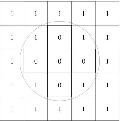
In the volume-penalising immersed boundary method adopted by Mikhal [2] geometries are respresented by immersing it in a Cartesian grid. A forcing term in the Navier-Stokes equations, which can be either switched ‘off’ and ‘on’ depending on whether the grid cell is in the ‘fluid’ or ‘solid’ part of the domain, ensures that there is no flow outside the geometry. Consider an example of a masking function of a circle on a grid with five cells in both the horizontal and the vertical direction, as seen in Figure 3.1. If a cell is entirely within the circle, it is treated as part of the fluid domain. Otherwise, it is labeled as part of the solid domain. In the fluid domain the masking function attains the value 0 and in the solid domain the value 1. Because this is a fairly simple case, it is readily checked whether a cell is entirely within the geometry. For other cases later on in this thesis, the only condition on whether a cell is ‘fluid’ or ‘solid’ is whether the cell centre is inside the geometry.

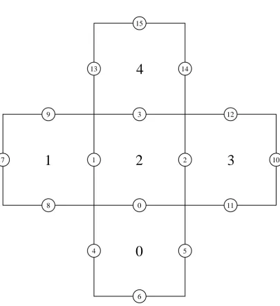
By removing the cells that are part of the solid domain, the number of cells is reduced in this example by 80%. For more complex geometries, which are quite slender and possibly highly 3D contorted, the reduction in the number of cells can amount to 95%, which could result in a significant reduction of the amount of time needed to compute velocity and pressure fields, especially for large cases. The ‘fluid’ cells are labeled, starting from 0. The labeling as shown in Figure 3.2 is just one way to do it. In principle, other choices can be accepted as well. The labeling of the faces is restricted by one of the conditions mentioned above. Internal faces are labeled first and the labeling finishes with boundary faces. For each cell the faces are checked and the faces without label are given a label. If a cell has two or more faces without a label, the face which connects to the cell with the lower label is labeled first.

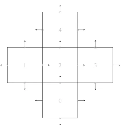
The face normal vectors are such that they point into the cell with the larger label for internal faces and outwards for boundary faces, as in Figure 3.3. The cell with the lower label is called

theowner of the face and the cell with the larger label is called theneighbour of the face.

Figure 3.4 shows the masking function as the grid is refined twice, where the number of cells is doubled in each direction with each refinement. ‘Solid’ cells are shown in black and ‘fluid’ cells are shown in white. Clearly, with only two refinements, already a quite acceptable approximation to the circle is achieved, which obviously improves further with increasing resolution.

3.2 Poiseuille flow

In this section Poiseuille flow through a pipe is considered. First, the setting and several flow parameters are presented. Second, velocity profiles for different resolutions are compared to the analytical solution. Third, the observed convergence is quantified with several mathematical measures.

Setting and control parameters

Flow through a pipe with radius R= 1 (m) and length Lx = 3 (m) with volumetric flow rate

Q= π₂ (m3_{/s), thus with average streamwise velocity ¯}_u₌ 1

2, and kinematic viscosity ν =

1

2 is

considered. This flow corresponds to a Reynolds number Re = 1. The analytical solution to the Navier-Stokes equation for this flow is

u(x, y, z) =R(1−y2−z2), v(x, y, z) =w(x, y, z) = 0. (3.1)

In order to simulate the flow the immersed boundary method is used as a starting point and

the pipe is considered to be immersed in a box of dimensions 3×3×3 (m), and a uniform grid is

(21)

15 3.2. Poiseuille flow

1

0

1

0

1

[image:21.595.72.490.159.581.2]

1

0

1

(22)

0

2

4

1

3

0 1

8 7

9

2 3

5 4

6

10

11 12

13 14

[image:22.595.113.519.146.590.2]

15

(23)

1

2

4

3

0

2

4 5

6

11

10 12

14 15

13

9

7

8

1

3

[image:23.595.73.489.155.583.2]

0

(24)

(a) (b) (c)

Figure 3.4: Illustration of the masking function as the grid is refined.

analytical, of the streamwise velocity uare shown. For k≥5 the numerical solution is already

visually close to the analytical solution and the approximation gets better askis increased. In

order to quantify the apparent convergence different ways to measure the distance between the numerical and analytical solution are introduced.

To check convergence the distance between the numerical solutions and the analytical solution

is measured with two different norms, i.e. thel2-norm

||uNz−u||2=

v u u t Nz X n=1

(uNz(0,0, zn)−u(0,0, zn))

2_, _(3.2)

wherezn is a grid point, which depends onNz, and thel∞-norm

||uNz −u||∞= max

n=1...Nz

|uNz(0,0, zn)−u(0,0, zn)|. (3.3)

In Figure 3.6 these distances are compared as a function ofNz. Clearly, both distances converge

with first order.

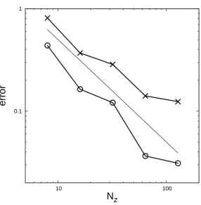
Being able to compare a numerical solution to an analytical solution is convenient but is often not possible for more complex geometries. For that reason, one might want to measure distances between a numerical solution and the analytical solution differently. Figure 3.7 shows how three different quantities converge to the exact value. Two lines, one showing the difference

in the diameter of the pipe, measured as the difference between z1 and zNz, and one showing

the difference between the integrals over the streamwise velocityu from z1 to zNz, where the

integral over the numerical solution is found with a trapezoidal rule, marked with crosses and circles respectively, indicate first order convergence. The difference in the maximum streamwise velocity, which is shown as a line with triangle markers, appears to converge faster with second order.

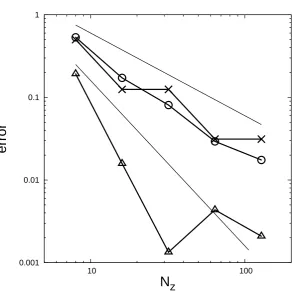
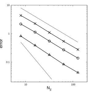
Instead of measuring distances over a line one could compare quantities related to the entire volume of the pipe. Figure 3.8 shows the differences in the volume of the pipe (crosses), the

volume integral over the streamwise velocityu(circles) and the volume integral over the kinetic

energyE= 1₂(u2+v2+w2) (triangles). The straight lines without markers have slope−1 and

(25)

-1 -0.5 0 0.5 1

0 0.5 1 1.5 2

z

[image:25.595.135.429.213.513.2]

u

Figure 3.5: Velocity profiles for Poiseuille flow through a pipe of radius R = 1 for several

resolutions. The number of grid points in thez-direction isNz = 2k, wherek= 3. . .7, marked

with pluses, crosses, stars, open and filled squares respectively. The solid line corresponds to the

(26)

0.1 1

10 100

error

[image:26.595.174.461.223.515.2]

N

_z

Figure 3.6: Convergence of the streamwise velocity for Poiseuille flow through a pipe of radius

R= 1 towards the analytical solution u(x,0, z) =R(1−z2_{) in both the}_l2_{-norm (crosses) and}

(27)

0.001 0.01 0.1 1

10 100

error

[image:27.595.135.432.209.503.2]

N

_z

Figure 3.7: Convergence of several quantities with respect to the exact value for Poiseuille flow

through a pipe of radius R= 1. The crosses correspond to the length of the line from bottom

to top of the pipe in thez-direction, the circles to the integral of the streamwise velocityuover

this line and triangles to the maximum streamwise velocity along this line. The straight lines

(28)

0.1 1 10

10 100

error

[image:28.595.174.461.207.504.2]

N

_z

Figure 3.8: Convergence of several quantities with respect to the exact value for Poiseuille flow

through a pipe of radiusR= 1. The crosses correspond to the volume of the pipe, the circles to

the streamwise velocityuintegrated over the volume of the pipe and the triangles to the kinetic

energyE integrated over the volume of the pipe, whereE=1₂(u2₊_v2₊_w2_{). The straight lines}

(29)

Chapter 4

Applications

In this chapter flow through more realistic geometries is considered. First laminar flow through curved vessels is considered in Section 4.1 and this section is concluded with flow through a real-istic geometry. In Section 4.2 flow with realreal-istic flow parameters is examined and a comparison is made with laminar flow.

4.1 Curved and realistic vessels

In this section laminar flow through several curved vessels is considered and is concluded with laminar flow through a realistic geometry which is constructed from a masking function obtained after manipulation of a 3DRA scan.

The centerline of the curved vessels in this section is described by the curve (xc(s), yc(s), zc(s))

xc= 12s, yc= 2, zc= 4 + 2sin(2π(s−

1

4)) + 2(1−) sin(2π(s

3₋1

4)), (4.1)

with skewness-parameter∈[0,1]. The reference case with = 1 is considered first. Two

addi-tional cases, with= 0.5 and= 0.25 respectively, are considered to try to explain unexpected

behavior of the solution in the reference case.

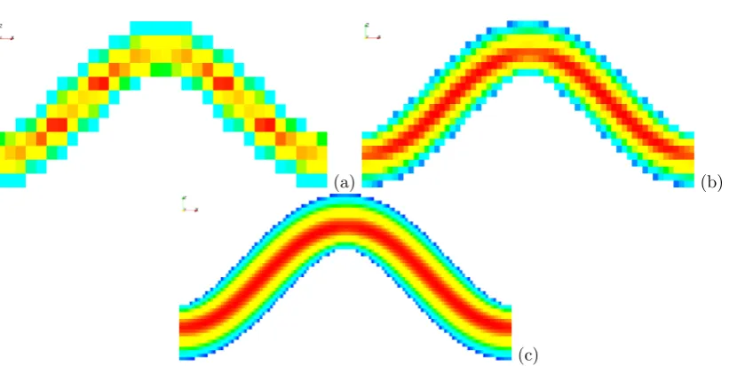
Figure 4.1 shows slices of the velocity field through the center of the vessel for three different

resolutions. At a coarse grid with resolution 32×8×16 the solution respresents the flow rather

poorly, but with one refinement to a resolution of 64×16×32 the solution shows qualitatively

agreement with the next refinement to a resolution of 128×32×64.

In Figure 4.2 an illustration of the masking function on a plane through the center of the vessel is given together with profiles of the streamwise velocity at different streamwise locations

at resolution 64×16×32. These velocity profiles look similar to what was found in [2].

For different resolutions profiles of the streamwise velocity at several equidistant streamwise locations are shown in Figure 4.3. Note that grids with different resolution do not have coinciding grid points, because OpenFOAM uses a collocated grid, which results in slightly different

stream-wise locations as the resolution is increased. As the resolution is increased from 32×8×16,

the profiles clearly converge when viewed graphically. To quantify the convergence, measures similar to those introduced in Chapter 3 are used. An analytical solution is not available for this case, so each value is compared to the value obtained on the grid with the highest resolution

of 512×128×256 instead. Convergence of the geometrical representation, as measured by the

length of lines from bottom to top of the vessel at different x can be seen in Figure 4.4. For

(30)

Chapter 4. Applications 24

(a) (b)

(c)

Figure 4.1: Slices of the velocity field through the center of a curved vessel with= 1. Resolutions

are (a) 32×8×16 (b) 64×16×32 (c) 128×32×64. Colors correspond to the magnitude of the

velocity vector, where blue corresponds to zero and red corresponds to the maximum velocity.

0 1 2 3 4 5 6 7 8

0 2 4 6 8 10 12

z

x (a)

0 1 2 3 4 5 6 7 8

0 2 4 6 8 10 12

z

[image:30.595.113.524.119.325.2]

x (b)

Figure 4.2: (a) Masking function on a plane through the center of a curved vessel with = 1.

(31)

25 4.1. Curved and realistic vessels

two locations this length does not change as the resolution is increased from 32×8×16, since

at these locations the outermost edges of the geometry coincide with grid points at the coarsest grid. At the other locations the length converges slightly faster than first order.

0 1 2 3 4 5 6 7 8

4 6 8 10 12

z

[image:31.595.141.425.154.441.2]

x

Figure 4.3: Velocity profiles on a plane through the center of a curved vessel with = 1.

Resolutions are ranging from 32×8×16 to 512×128×256, where the number of grid cells

is doubled in every direction with each refinement, indicated by dots, dash-dot-dot, dash-dot, dashed and solid lines respectively.

Figure 4.5 shows the error of the integral of the streamwise velocity over lines from bottom to top of the vessel with respect to the value of the integral for a solution found on a grid

with resolution 512×128×256. The error clearly shows second order convergence and at some

locations even higher order convergence is achieved.

The maximum streamwise velocity along lines from bottom to top of the vessel converges with second or even higher order, as can be seen in Figure 4.6. At two locations this maximum

value gets very close to the maximum value found on a grid with resolution 512×128×256.

Integrals over the entire volume of the vessel are also considered. In Figure 4.7 the error with

respect to the value at resolution 512×128×256 of the volume of the vessel, the volume integral

of the streamwise velocity and the volume integral over the kinetic energyE can be seen. These

three quantities show convergence which is close to second order.

By chosing = 0.5 the vessel becomes slightly skewed. This skewness presents a problem.

Although the centerline of the vessel is nicely periodic, the currently generated boundary is not. Extension of the geometry with a mirrored geometry solves this problem and a new geometry

(32)

0.1

10

error

[image:32.595.174.462.211.503.2]

N

_z

Figure 4.4: Error with respect to the numerical solution of the flow through the curved vessel

with = 1 at resolution 512×128×256 of the length of the line from bottom to top in the

z-direction at different streamwise locations xk = (kN₄x − 1₂)_NLx_x, k = 1. . .4, where Lx = 12.

The straight lines without markers have slope−1 and−2 respectively. Fork= 1,3 (crosses and

(33)

0.0001 0.001 0.01 0.1

10

error

[image:33.595.130.438.200.503.2]

N

_z

with= 1 at resolution 512×128×256 of the streamwise velocityuintegrated over the line from

bottom to top in thez-direction at different streamwise locationsxk= (kN₄x−1₂)L_Nx

x,k= 1. . .4,

marked with crosses, circles, triangles and diamonds respectively, whereLx = 12. The straight

(34)

1e-05 0.0001 0.001 0.01 0.1

10

error

[image:34.595.166.469.210.503.2]

N

_z

with= 1 at resolution 512×128×256 of the maximum value of the streamwise velocity along

the line from bottom to top at different streamwise locations xk = (kN₄x −1₂)L_Nx

x, k = 1. . .4,

marked with crosses, circles, triangles and diamonds respectively, whereLx= 12. The straight

(35)

0.01 0.1 1

100

error

[image:35.595.125.423.170.504.2]

N

_x

with = 1 at resolution 512×128×256 of the integralR

V1dV (crosses), the integral

R

V u dV

(circles) and the integral R_V E dV (triangles), where E = 1₂(u2+v2+w2). The straight lines

(36)

[image:36.595.110.527.162.431.2]

Figure 4.8, which clearly shows how the new geometry is formed from the original geometry and

a mirrored geometry. Similar to the case with= 1, the solution is poor at a coarse grid, but

after refining the grid once good agreement can be seen with the solution which is found when the grid is refined even further.

(a)

(b)

(c)

Figure 4.8: Slices of the velocity field through the center of a curved vessel with = 0.5.

Resolutions are (a) 32×8×16 (b) 64×16×32 (c) 128×32×64. Colors correspond to the

magnitude of the velocity vector, where blue corresponds to zero and red corresponds to the maximum velocity.

Figure 4.9 shows the masking function and profiles of the streamwise velocity at several streamwise locations on a plane through the center of the vessel. These profiles look similar to

the profiles which were found for the case with= 1.

In Figure 4.10 profiles of the streamwise velocity for different resolutions, ranging from 32×

8×16 to 512×128×256, at several equidistant streamwise locations are shown. At each location

the profiles appear to converge.

Figure 4.11 shows the error of the integral of the streamwise velocity over the lines from

bottom to top of the vessel with respect to the value of the integral at resolution 512×128×256.

This integral clearly converges with second order, where convergence seems to be somewhat faster at locations where the profiles are more symmetrical.

The maximum value of the streamwise velocity along the lines from bottom to top of the vessel seems to behave in a similar way. As can be seen in Figure 4.12 these values also converge

with second order with respect to the value at resolution 512×128×256.

(37)

31 4.1. Curved and realistic vessels 0 1 2 3 4 5 6 7 8

0 2 4 6 8 10 12

z x (a) 0 1 2 3 4 5 6 7 8

0 2 4 6 8 10 12

z

[image:37.595.133.419.345.628.2]

x (b)

Figure 4.9: Velocity profiles on a plane through the center of a curved vessel with= 0.5. The

resolution shown here is 64×16×32.

1 2 3 4 5 6

4 6 8 10 12

z

x

Figure 4.10: Velocity profiles on a plane through the center of a curved vessel with = 0.5.

Resulotions are ranging from 32×8×16 to 512×128×256, where the number of grid cells

(38)

0.0001 0.001 0.01 0.1 1

10

error

[image:38.595.166.468.209.509.2]

N

_z

Figure 4.11: Error with respect to the numerical solution of the flow through the curved pipe

with = 0.5 at resolution 512×128×256 of the integral R

IN(xk)u dz for xk = (

kNx

4 −

1

2)

Lx

Nx,

k = 1. . .4, marked with crosses, circles, triangles and diamonds respectively, where Lx = 12.

(39)

0.0001 0.001 0.01 0.1 1

10

error

[image:39.595.128.435.208.503.2]

N

_z

with= 0.5 at resolution 512×128×256 of the maximum value of the streamwise velocity along

the line from bottom to top of the vessel for different streamwise locations xk = (kN₄x −1₂)_NLx

x,

k = 1. . .4, marked with crosses, circles, triangles and diamonds respectively, where Lx = 12.

(40)

observed for the case with= 1.

0.01 0.1 1

100

error

[image:40.595.173.463.127.413.2]

N

_x

with= 0.5 at resolution 512×128×256 of the integralR

V 1dV (crosses), the integral

R

V u dV

(circles) and the integralR_V E dV (triangles), where E = 1₂(u2+v2+w2). The straight lines

without markers have slope−1 and−2 respectively.

With= 0.25 the vessel becomes even more skewed. Also with this case a mirrored geometry

is used as extension to the original geometry to obtain periodicity in thex-direction. Figure 4.14

shows slices of the velocity field through the center of the vessel. Typical behavior is observed,

where starting from a coarse grid with resolution 32×8×16 the solution obtained after one

refinement shows qualitative agreement with the solution at even finer grids.

In Figure 4.15 the masking function and profiles of the streamwise velocity on a plane through the centre of the vessel are shown. The increased skewness creates a fairly sharp transition in the geometry, as can be seen from the masking function, but this does not seem to affect the solution in a dramatic way at the selected flow conditions.

Profiles of the streamwise velocity at equidistant streamwise locations are shown in Fig-ure 4.16. The profiles clearly converge. Even at locations where the geometry changes rapidly, convergence seems to be fairly good.

Convergence of the integral of the streamwise velocity over the line from top to bottom for several streamwise locations is clearly second order, as can be seen in Figure 4.17. The rate of

convergence of the error with respect to the value of the integral at resolution 512×128×256

seems to depend less on the location than for the previous two cases.

(41)

(a)

(b)

(c)

Figure 4.14: Slices of the velocity field through the center of a curved vessel with= 0.25 with

= 0.25. Resolutions are (a) 32×8×16 (b) 64×16×32 (c) 128×32×64. Colors correspond

to the magnitude of the velocity vector, where blue corresponds to zero and red corresponds to the maximum velocity.

0 1 2 3 4 5 6 7 8

0 2 4 6 8 10 12

z

x (a)

0 1 2 3 4 5 6 7 8

0 2 4 6 8 10 12

z

[image:41.595.74.491.100.395.2]

x (b)

Figure 4.15: Velocity profiles on a plane through the centre of a curved vessel with= 0.25. The

(42)

1 2 3 4 5 6

4 6 8 10 12

z

[image:42.595.175.461.224.517.2]

x

Figure 4.16: Velocity profiles on a plane through the center of a curved pipe with = 0.25.

Resolutions are ranging from 32×8×16 to 512×128×256, where the number of grid cells are

(43)

0.001 0.01 0.1

10

error

[image:43.595.132.433.216.502.2]

N

_z

with = 0.25 at resolution 512×128×256 of the integral R

IN(xk)u dz for xk = (

kNx

4 −

1

2)

Lx

Nx,

k= 1. . .4, marked with crosses, circles, triangles and diamonds respectively, whereLx= 12. All

lines seem to indicate second order convergence. The straight lines without markers have slope

(44)

512×128×256 seems to give the same conclusion as the error of the integral of the streamwise

velocity. As can be seen in Figure 4.18, the maximum streamwise velocity converges with second order, and at one location even with higher order.

0.0001 0.001 0.01 0.1 1

10

error

[image:44.595.167.467.157.436.2]

N

_z

with = 0.25 at resolution 512×128×256 of the maximum value of the streamwise velocity

along a line from bottom to top for streamwise locationsxk = (kN₄x −1₂)_NLx_x,k= 1. . .4, marked

with crosses, circles, triangles and diamonds respectively, where Lx = 12. The straight lines

The errors of the integrals over the entire volume of the vessel with respect to the value at

resolution 512×128×256, which are presented in Figure 4.19, very clearly show second order

convergence.

With these three cases it was shown that it is possible to simulate laminar flow in curved vessels, even if they are skewed. Results in terms of profiles and convergence of different quantities are convincing enough to assume that it is possible to simulate laminar flow in realistic geometries as well.

4.2 Realistic geometry and flow conditions

(45)

39 4.2. Realistic geometry and flow conditions

0.01 0.1 1 10

100

error

[image:45.595.135.429.208.509.2]

N

_x

with= 0.25 at resolution 512×128×256 of the integralR

V 1dV (solid), the integral

R

V u dV

(dashed) and the integral R_V E dV (dotted), where E = 1₂(u2+v2+w2). The bold lines have

(46)

by looking at streamlines and contour plots of the streamwise velocity, a convergence study is done for the laminar flow. It will become clear that convergence is much harder to achieve for the realistic flow.

The vessel under consideration has radius R = 1.94·10−3_{(m), a typical value for a vessel}

in the circle of Willis, the mayor system supplying blood to the brain. The kinematic viscosity

of blood isν = 3.01·10−6 (m2/s). Figure 4.20 shows streamlines of laminar flow with average

streamwise velocity ¯u= 1.55·10−3(m/s) through the vessel, corresponding to a Reynolds number

[image:46.595.108.523.237.470.2]

Re = 1. The streamlines indicate that the main flow does not enter the cavity of the aneurysm at the selected flow condition.

Figure 4.20: Streamlines of laminar flow through a geometry constructed from a masking

func-tion, which was obtained after manipulation of a 3DRA scan, at resolution 256×128×256.

In Figure 4.21 the streamlines of realistic flow with average streamwise velocity ¯u= 0.388

(m/s) is shown, corresponding to Re = 250. The behavior of the flow changes drastically,

compared to Re = 1. Streamlines now do enter the cavity of the aneurysm and the flow appears to become somewhat unsteady, even in parts of the domain where the geometry changes smoothly. Contour lines of the streamwise velocity of laminar flow at two different locations, one being in the part of the domain where the geometry changes smoothly and one near the opening of the cavity of the aneurysm, are shown in Figure 4.22. Both in Figure 4.22(a) and the lower part of Figure 4.22(b) a flow reminiscent of Poiseuille flow can be recognised. Figure 4.22(b) also confirms that the main flow does not enter the cavity of the aneurysm. The solutions seems to

converge relatively fast, the contour lines at resolution 128×64×128 look a lot like the contour

lines at resolution 256×128×256.

(47)

[image:47.595.75.486.99.337.2]

Figure 4.21: Streamlines of flow at Re = 250 through a geometry constructed from a masking

function, which was obtained after manipulation of a 3DRA scan, at resolution 256×128×256.

streamwise direction and small areas of backflow appear at the top of the vessel. In Figure 4.23-(b) a large area of backflow can be recognised at the top of the vessel, while areas of flow in the streamwise direction are mainly at the bottom and at the right side of the vessel.

In Figure 4.24 profiles of the streamwise velocity of laminar flow through the vessel are shown. The convergence of the solution, which dominates especially in the smooth part of the domain, can be very clearly seen in this figure.

When looking at profiles of the streamwise velocity in the developing phase of realistic flow through the vessel, as can be seen in Figure 4.25, it is clear that the solution indeed converges rather poorly. However, certain features of the flow can be recognised over different resolutions. The locations of extreme values are approximately the same for different resolutions.

The convergence of the profiles of the streamwise velocity that was observed for laminar flow also becomes apparent in Figure 4.26, which shows that the integral over the streamwise velocity and the maximum streamwise velocity converge with second or higher order.

The volume of the vessel and the integrals of the streamwise velocity and kinetic energy over the volume of the vessel very clearly converge with second order, as can be seen in Figure 4.27.

Although the profiles of the streamwise velocity of realistic flow showed very little convergence, the integral of the streamwise velocity over a line in the smooth part of the domain still converges with second order, as can be seen in Figure 4.28. The integral of the streamwise velocity over a line near the opening of the cavity of the aneurysm and the maximum streamwise velocity along these lines converge with an order which is much closer to first order.

(48)

(a)

[image:48.595.119.516.218.504.2]

(b)

Figure 4.22: Contour lines of the streamwise velocity of laminar flow on cross sections in the

y−zplane at 1/16th (a) and half (b) of the domain in thex-direction. The values of the contour

lines in (a) are uniformly distributed on the interval [0,6.30·10−3] and in (b) on the interval

[−7.53·10−6,4.58·10−3]. From left to right the resolutions are 64×32×64, 128×64×128 and

(49)

(a)

(b)

Figure 4.23: Contour lines of the streamwise velocity of realistic flow with Re = 250 on cross

sections in they−zplane at 1/16th (a) and half (b) of the domain in thex-direction at resolution

256×128×256. The values of the contour lines in (a) are uniformly distributed on the interval

[−0.292,2.16] and in (b) on the interval [−0.909,1.42]. From left to right time increases from

0.01 to 0.4 with increment ∆t= 0.13.

2 2.5 3 3.5 4

0 0.5 1 1.5 2 2.5 3 3.5 4

z

u (a)

5.5 6 6.5 7 7.5 8 8.5

0 0.5 1 1.5 2 2.5

z

[image:49.595.76.485.118.335.2]

u (b)

Figure 4.24: Profiles of the streamwise velocity in dimensionless quantities of laminar flow at

1/16th of the domain in thex-direction and 13/16th of the domain in they-direction (a), and at

half of the domain in both thex-direction and they-direction (b). Resolutions are 32×16×32

(50)

Chapter 4. Applications 44 2 2.5 3 3.5 4

0 1 2 3 4

z u (a) 5.5 6 6.5 7 7.5 8 8.5

-2 -1 0 1 2 3 4

z

u (b)

Figure 4.25: Profiles of the streamwise velocity in dimensionless quantities in the developing

phase, att= 0.01, of realistic flow with Re = 250 at 1/16th of the domain in thex-direction and

13/16th of the domain in the y-direction (a), and at half of the domain in both thex-direction

and they-direction (b). Resolutions are 32×16×32 (dots), 64×32×64 (dash-dot), 128×64×128

(dash) and 256×128×256 (solid).

1e-08 1e-07 1e-06 1e-05 10 error N_z (a) 1e-05 0.0001 0.001 10 error N_z (b)

Figure 4.26: Error with respect to the numerical solution of laminar flow through the vessel at

resolution 256×128×256 on lines from bottom to top of the vessel at 1/16th of the domain in

thex-direction and 13/16th of the domain in they-direction (crosses), and at half of the domain

in both the x-direction and the y-direction (circles). In (a) the error of the integral of the

streamwise velocity over the lines is shown and (b) shows the error of the maximum streamwise

(51)

1e-13 1e-12 1e-11 1e-10 1e-09 1e-08 1e-07

100

error

[image:51.595.132.432.208.509.2]

N

_x

Figure 4.27: Error with respect to the numerical solution of laminar flow through the vessel at

resolution 256×128×256 of the integral R

R

V u dV (circles) and

the integralR_V E dV (triangles), whereE=1₂(u2+v2+w2). The straight lines without markers

(52)

0.0001 0.001

10

error

N_z

(a)

0.1 1

10

error

N_z

(b)

Figure 4.28: Error with respect to the numerical solution of realistic flow at Re = 250 through

the vessel at resolution 256×128×256 on lines from bottom to top of the vessel at 1/16th

of the domain in the x-direction and 13/16th of the domain in the y-direction (crosses), and

at half of the domain in both thex-direction and the y-direction (circles). In (a) the error of

the integral of the streamwise velocity over the lines is shown and (b) shows the error of the

maximum streamwise velocity along the lines. The straight lines without markers have slope−1

and−2 respectively.

When comparing the average pressure drop over the vessel for laminar and realistic flow in Figure 4.30, a significant difference in temporal behavior can be seen. After a short period of highly oscillatory behavior associated with the transient following the unrealistic initial condition of zero flow, the global pressure gradient stabilises and remains constant for laminar flow, whereas the global pressure gradient for realistic flow continues with a lower amplitude oscillation.

The initial errors for each of the components of the fluid velocity in the iterative method to solve the momentum equations are shown in Figure 4.31. The termination criterion for the

iterative method requires that this error is lower than 10−5_{. Even after this criterion is met by}

(53)

1e-08 1e-07

100

error

N

_x

Figure 4.29: Error with respect to the numerical solution of realistic flow at Re = 250 through

the vessel at resolution 256×128×256 of the integral R

R

V u dV

(circles) and the integral R_V E dV (triangles), where E = 1₂(u2+v2+w2). The straight lines

34 34.5 35 35.5 36 36.5 37 37.5 38

0.1 1

pressure gradient

t (a)

0 0.5 1 1.5 2

0.0001 0.001 0.01 0.1

pressure gradient

[image:53.595.132.432.106.390.2]

t (b)

Figure 4.30: Evolution of the global pressure gradient in the streamwise direction, shown in dimensionless quantities, at different resolutions for both laminar flow (a) and realistic flow (b).

(54)

1e-09 1e-08 1e-07 1e-06 1e-05 0.0001 0.001 0.01 0.1 1

1 10 100 1000

residual

iteration (a)

1e-05 0.0001 0.001 0.01 0.1 1

1 10 100 1000 10000 100000 1e+06

residual

iteration (b) Figure 4.31: Initial errors in the iterative method to solve the momentum equations for each

time step of the velocity in thex-direction (solid), y-direction (dashed),z-direction (dash-dot)

(55)

Chapter 5

Discussion and outlook

The main goal of this project was to simulate blood flow in the human brain with OpenFOAM. The immersed boundary (IB) method has proven to be a suitable method for these type of simulations. With the IB method, a geometry is simply immersed in a Cartesian grid and is respresented by means of a masking function. This masking function is a binary function which equals zero if a grid cell is part of the geometry and one otherwise. While complex and time consuming grid generation is prevented, the simplicity of the IB method is in itself a disadvantage. Namely, often only a small portion of the grid cells are part of the geometry, which makes the IB method a rather inefficient method in terms of computation time. In this project an effort was made to construct a grid in OpenFOAM from the masking function, including only grid cells which are part of the geometry. To construct the grid, OpenFOAM requires a number of input files. The challenge was to extract the grid cells which are part of the geometry from the masking function in an efficient way and generate the input files accordingly. This was done succesfully and the most important requirements posed by OpenFOAM on the input files were presented in this thesis.

To validate the approach in this thesis, Poiseuille flow through a cylindrical pipe was con-sidered. As expected, a first-order convergence of the numerical solution was observed. This corresponds to what was found by Mikhal [2]. When laminar flow through a curved pipe was also examined, the numerical solution showed an unexpected second-order convergence. In the study by Mikhal this superconvergence, which was attributed to the symmetry of the domain in this thesis, was not observed. Attempts to recover first-order convergence by increasing the skewness of the curved pipe, thus breaking symmetry, did not succeed. The superconvergence of the numerical solutions for curved pipes deserves further attention. Results from simulations of flow through these model geometries were convincing enough to assume that simulations of laminar flow through a realistic geometry, which was extracted from 3D rotational angiography (3DRA) data, would give reliable results as well. Indeed, the resulting numerical solutions be-haved as expected and showed no abnormalities. Velocity profiles at different locations in the blood vessel even suggested a second-order convergence. Simulations at higher resolutions could confirm this. Naturally, the resolution of the grid is limited by the resolution of the original 3DRA data. Simulations of flow at physiological flow rates revealed unsteady behavior of the flow. This is a remarkable result, since Mikhal explicitly reports steady flow at these flow rates. The current approach can be improved upon in several ways. The staircase approximation of the geometry led to first-order, and even second-order, convergence of the numerical solution. It would be an interesting topic of research to do a similar study with a smoothened geometry, e.g. by adding cells with a prism shape. A crucial part in further development of the currently

(56)

Chapter 5. Discussion and outlook 50

(57)

Bibliography

[1] R.I Issa. Solution of the implicitly discretised fluid flow equations by operator-splitting.

Journal of Computational Physics, 62(1):40 – 65, 1986.

[2] Julia Mikhal. Modeling and simulation of flow in cerebral aneurysms. PhD thesis, University

of Twente, Enschede, October 2012.

[3] OpenFOAM Foundation. OpenFOAM Programmer’s guide, May 2012. Version 2.1.1.

Flow prediction in brain aneurysms using OpenFOAM