1
Faculty of Electrical Engineering,
Mathematics & Computer Science
Implementation of Digital Class - D
amplifier controller in C
λ
aSH
Anirudh Gottimukkala M.Sc. Thesis November 2017
Supervisors:
List of acronyms
ADC Analog to Digital Converter
CD Compact Disk
CIFF Cascaded Integrators with Feed Forward summation DAC Digital to Analog Converter
DSP Digital Signal Processing FIR Finite Impulse Response
HDL Hardware Descriptive Language IIR Infinite Impulse Response PCM Pulse Code Modulated PWM Pulse Width Modulator
NPWM Natural PWM
NTF Noise Transfer Function RTL Register Transfer Level SNR Signal to Noise Ratio STF Signal Transfer Function
UPWM Uniform PWM
VHDL Very High speed IC Hardware Descriptive Language
Acknowledgements
I would like to thank the following people, who had supported me in my course of this re-search.
• Simon - Thijs de Feber for being my teacher, guide and a patient listener, whose advice
on taking steps one at a time was very essential.
• Tim van Doesum for helping me a lot with MATLAB scripts and guiding me with my
crucial progress in the final stages.
• Judy and Tim for hosting very nice dinners and for our usual meetings and celebrations.
• Daniel Schinkel for his inputs and patience for pedantic queries.
• Axign, for their continuous trust and support for more than a year.
• Professor Andre Kokkeler and Professor Jan Kuper for their continuous trust and
ac-ceptance.
And finally, my parents back in India and my cousin in Eindhoven for having faith in me and for their blessings.
- Anirudh Gottimukkala
Abstract
In this thesis a new way of implementing a Class - D amplifier controller is presented. A Class - D amplifier controller is a system that essentially performs Sigma - Delta modulation to quantize discrete digital input into a 1 - bit Pulse Width modulated signal that is used to drive a power amplifier. The system has internal control loops that perform the necessary noise filtering thus providing quantization noise - free modulated output. This system in a digital implementation traditionally follows digital design flow starting from a VHDL descrip-tion, which can be time consuming for a controller design that has a greater complexity.
The approach investigated in this thesis involves modeling of the system in a functional programming language Haskell. In the model, elementary mathematical equations that are used to describe the system are modeled in the form of higher order functions. The Haskell code is then converted to a CλaSH (CAES Language for Synchronous Hardware) code,
which is a sub-set of Haskell that is used to describe sequential digital hardware. The con-version involves minor changes to the base Haskell model. With its native compiler, CλaSH
is used to generate VHDL code from the Haskell modelled system.
Simulations are performed on Haskell and CλaSH models and compared with the
simu-lation of an equivalent Simulink model. The comparison shows that the CλaSH
implemen-tation respects the intended functionality of the system.
Contents
List of acronyms iii
Acknowledgements v
Abstract vii
1 Introduction 3
1.1 Objectives of research . . . 4
1.2 Structure of Thesis . . . 5
2 Background 7 2.1 Digital Audio . . . 7
2.2 Introduction to Haskell . . . 8
2.2.1 Recursive definitions . . . 9
2.2.2 Functional Hardware Descriptive Languages (FHDL) . . . 10
2.3 Pulse Width Modulation Amplifier . . . 10
2.4 Class - D Amplifier Controller . . . 17
2.4.1 Mathematical modeling . . . 17
2.5 Functional Hardware Descriptions in Haskell . . . 21
2.5.1 Modeling in Haskell . . . 21
2.6 Conclusions . . . 29
3 Implementation in CλaSH 31 3.1 Introduction . . . 31
3.1.1 Data types and conversions . . . 32
3.1.2 Closed loop system . . . 35
3.2 Conclusions . . . 36
4 Results and Comparisons 37 4.1 Haskell Simulation . . . 38
4.2 CλaSH Simulation . . . 38
4.3 Synthesis . . . 42
4.4 Conclusions . . . 43
5 Conclusions 45
6 Future Work 47
Bibliography 49
A Appendix A 51
A.1 VHDL Code for cdAmp entity . . . 51
A.2 VHDL Code for cdAmp top level. . . 51
A.3 VHDL Code for lfilter . . . 53
A.4 VHDL Code for pwm . . . 56
Chapter 1
Introduction
Among many applicative areas of signal processing, audio is perhaps one of the most in-teresting and challenging fields. Right from recording of the source, processing and repro-duction of the original audio source, there are many stages and intricate steps involved to achieve a pure audio reproduction. Over time, audio systems dedicated to an efficient audio reproduction moved away from the traditional analog domain to digital, proving faster pro-cessing rates and much better elimination of noise in the audio band.
An audio amplifier is an electronic system that reinforces low power auditory signal such that it is strong enough to drive a power load, in this case a loudspeaker. Most audio am-plifiers are analog devices, in the sense that the signal is in the from of an analog wave. However, amplifying audio from a digital source requires digital to analog conversion. A class of amplifier suitable for such a task is the Class - D amplifier, which operates on Pulse-Width Modulation (PWM) of audio samples. The amplifier drives a switching power stage to fully ON or fully OFF states, hence giving a theoretical efficiency of 100%. A purely digital solution of this class is therefore faster and efficient.
The design of digital systems start with a general specification of the system with re-spect to its operational characteristics, energy efficiency, speed of operation and resources consumed, notably among many more. In the next step, the specifications are translated in hardware descriptive languages like VHDL or Verilog. Synthesis tools have been developed that can derive a gate-level hardware implementation of a digital system from a behavioral description in a Hardware Descriptive code (HDL).
The traditional hardware descriptive languages mentioned previously fall short when de-velopment time is a crucial factor. Depending on the demands , the system can be quite complex, making the development process much time consuming and error-prone. Hence, the need for a higher level of abstraction is imminent, making the designer focus more on the behavioral aspects and let the tool handle the implementation. To achieve a greater abstraction, functional programming is preferred. In a functional style of programming, the behavior is described as mathematical equations or abstract definitions in the form of basic
functions, and function calls will eventually describe the intended system. The advantage of such abstraction is that the system description is more concise, short and less error prone, and more importantly the development time of complex systems gets much shorter.
A tool that generates fully synthesizeable VHDL code from a specification written in the functional programming language Haskell exists, developed by CAES group in University of Twente. This tool is called CAES Language for Synchronous Hardware design (CλaSH),
and it gives the opportunity to describe a system at a high abstraction level by describing its mathematical properties using functional expressions. By describing a problem description in a functional programming language, the simulations on the system can be done without any transformations to a programming language with other semantics. The direct transfor-mation from the description in CλaSH to a hardware description in VHDL also eliminates the
need for a manual conversion step which can introduce errors in the system.
In this research, a simple Class - D amplifier controller is modeled and implemented in CλaSH. The way to implementation first goes through modeling the required system in
Haskell and subsequently implementation in CλaSH. Simulations are performed in their
re-spective native environments to evaluate the correctness and also the performance results, since it will be a point of interest in answering the question:
Is CλaSH a suitable language and environment to design application specific signal processing systems?
1.1 Objectives of research
The primary objective of this research is a demonstration of how a digital Class-D amplifier controller can me implemented in CλaSH. As a start, the system is first modeled in Haskell
and eventually translated to CλaSH code. Finally, the extent at which CλaSH can be
em-ployed to implement complex architectures can be established.
It is shown that linearity of Class - D operation increases with increasing the sampling rate of the system [1]. However, problems associated with sample rate increase arise during an attempt to obtain a high resolution audio signal. To circumvent this issue, DSP techniques like noise shaping is employed, which is a process by which noise in audio band is reduced while using a low resolution modulator, while using a slower clock speed. This technique is described in Sigma - Delta (Σ∆) Modulation theory.
Concepts of sample rate conversion is quintessential in digital signal processing (DSP) operations, however, these concepts will be briefly described in theory and not as a part of implementation. The research contains following points of discussion:
1.2. STRUCTURE OFTHESIS 5
• Implementation of the architecture in the Functional Hardware Descriptive Language
(FHDL) CλaSH.
• Evaluating simulation response of CλaSH with a reference Haskell model, and
• Analyzing synthesis results of CλaSH generated VHDL description of the system.
Analysis of imperfections caused in this system is not discussed as the central point of this research is implementation. However, improvements associated with the system can be a topic of future development.
1.2 Structure of Thesis
The structure of this thesis is presented below.
Chapter 2 gives a brief introduction of digital audio. A general signal chain of audio recording to reproduction is presented. Further explanation is given about Pulse Width Modulator (PWM) amplifiers and their internal workings. Major focus is given on the concept of noise shaping and determination of an optimal noise shaper. The last part of the chapter focuses on modeling the Class - D amplifier controller mathematically and in functional pro-gramming language Haskell. This step lays the foundation for implementing the system in CλaSH, which is the primary focus of this research.
Chapter 3 introduces CλaSH as a Functional Hardware Descriptive Language (FHDL).
A brief introduction to its similarities with Haskell and advantages of designing digital hard-ware is presented. Steps necessary to translate Haskell model into CλaSH implementation
is laid out. Concluding remarks include the similarities with Haskell and intuitive reasoning of system implementation.
Chapter 4 compares simulation results of Haskell and CλaSH implementations. A
quan-titative proof is presented and comparisons are made between outputs of each implemen-tation. Furthermore, the results of Haskell and CλaSH models are compared against a
Simulink model to establish feasibility and verity of modeling the system in functional envi-ronment.
Chapter 2
Background
This chapter introduces a brief background on digital audio formats along with a standard digital audio system chain. Furthermore, sections are dedicated to mention the theory of a Class - D amplifier. Also included are fundamentals of Haskell, a functional programming language and CλaSH, which is a functional language for describing synthesizable digital
hardware in a functional paradigm.
2.1 Digital Audio
Digital audio is a format that is used for sound recording and reproduction, where analog signals are recored into a digital format. Digital audio over time has replaced analog record-ing and reproduction techniques in view of its efficiency and speed.
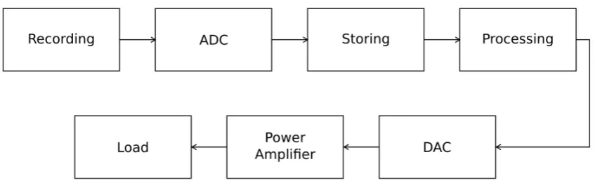
Digital audio processing systems require input in the form of digital encoded values of sampled analog signals. A digital audio system thus starts first with sound converted into an analog signal by a microphone. The analog signal is then encoded into a digital signal by using an Analog - to - Digital converter (ADC). Normally, a digital signal is a Pulse - Code Modulated (PCM) signal that has a resolution depending on the resolution of the ADC which is used. In typical digital audio systems, the resolution used is 16 - bit, and the audio sig-nal is sampled at 44.1 kHz, which gives 44100 samples per second, in case of CD audio. For other formats, different sampling frequencies and resolutions exist. With common digital tools and techniques, the encoded digital values can be stored and/or processed. To output the processed signal, a Digital - to - Analog converter (DAC) is used to obtain an analog equivalent of the digital signal, which is then passed through a power amplifier and given to a loudspeaker or headphones. The entire process of recording to reproducing an audio signal can be visualized in an audio reproduction chain as shown in Figure 2.1.
Figure 2.1: Audio recording and reproduction chain
2.2 Introduction to Haskell
A functional programming language, or paradigm, utilizes functions. Executions and calcu-lations are performed by calling functions, that build the required structure. In other words, program execution happens by constant evaluation of expressions that are defined in the said functions. For instance, a function can call another primitive function to evaluate one of its arguments, the result of which is used to evaluate another internally defined operation. One such language is Haskell, which builds the basis for CλaSH in this research.
In imperative languages like C, operations are performed by giving the computer a series of tasks and executions are handled by the computer. Most expressions are evaluated in an ’implied’ fashion, that means the program has an internal state and the state can change. For example, a variable can have an initial value, and the same variable can be put into an expression that makes it increment by a value. In a pure functional environment how-ever, the computer or program can only be told what the assignments are. For example, a function defined to calculate a sum of all numbers in a list needs to be told what that list is as an argument, and it results in an evaluated value. Also, the function is guaranteed to return the same value if called with the same argument. This has an advantage, in that the function lacks side - effects. The intended behavior is thus proven at any point of time [2].
A famous attribute of Haskell is it’s laziness. A Haskell program does not evaluate func-tions and provide results unless called otherwise. This is also known as the ’lazy evaluation strategy’, which delays the evaluation of an expression until its value is needed. By this strategy, control flow is more abstracted and possibly infinite data structures can be defined. Furthermore, unnecessary calculations can be avoided with lazy evaluation, thus increasing performance of programs [2].
2.2. INTRODUCTION TOHASKELL 9
error reporting, which means debugging is quick as common errors are identified at compile time.
2.2.1 Recursive definitions
An important advantage of describing architectures in functional programming is that func-tional paradigm supports higher order functions and recursive definitions. From a hardware descriptive point of view, a higher order function could for example be composed of a direct mathematical relation that is instantiated in another function, and so on. A mathematical relation can be anything from a simple adder to modules like full adders that can be called in a carry look-ahead adder structure. With each adder (in this example) having the same mathematical relation inside them, the model becomes more concise and easier to debug. While this is straightforward for combinatorial logic, sequential logic needs to be tackled in a different way in a functional environment, since it does not support loops like imperative environments.
Recursive modeling is the backbone of any Functional Hardware Descriptive Language (FHDL). Most digital designs are evidently sequential, with internal states keeping track of states of data at every clock tick. In an imperative way, they can be modeled simply by formulating a loop with the required number of iterations and the loop takes care of itera-tions implicitly. Functional languages like Haskell, however, evaluate things differently in this respect, as the evaluation is lazy and functions are pure, i.e, every evaluation with a same input gives the same output. Hence, a sense of previous state has to be introduced. This can be done again with the help of higher order functions, created solely for the purpose of ”storing” a previously calculated value.
A simple example to consider for demonstrating this strategy can be a mealy machine. In a mealy machine, the present output depends on the present input and a previously cal-culated output, which can be a result of any combinatorial (or mathematical) calculation, for example an accumulator. To model an accumulator in Haskell, two functions are to be declared, one that contains the actual mathematical (combinatorial) addition and the state for one computation, and another to recursively call the previously defined function. Listing 2.1 illustrates the example in Haskell, which models an accumulator.
In this simple code, the functionaccis modeled to have a statesand an inputaas
argu-ments, and result a tuple of next states0 and present outputyas (s0, y). Functionsimulate
is also defined that calls any functionf, initial statesand an input listas as arguments. A
case can now be considered when runningsimulatewithf asacc. It outputs a valueyand
then calls itself again with argumentsacc, updated states0 resulting from function evaluation
Important point to note here is how the next states0 ofsimulate is mapped to the next
state s0 ofacc. Since the next states0 is simplyy, the next state definition becomess0 =y.
When recursively callingsimulatewiths0,s0 takes on the valueyand maps it to the present
state, and the process repeats. When simulated with a list ranging from 1 to 10, the result is a list with accumulated additions, characteristic of an accumulator. In this way, a state ma-chines can be realized and this fundamental behavior of recursive calling forms an important base for definingmealyfunction in CλaSH, which will be discussed later.
1 acc s a = (s’,y)
2 where
3 y = s + a
4 s’ = y
5
6 simulate f s (a:as) = y : simulate f s’ as
7 where
8 (s’,y) = f s a
Listing 2.1: Haskell definition of an accumulator
2.2.2 Functional Hardware Descriptive Languages (FHDL)
Haskell’s features like lazy evaluation, recursive definition and polymorphism could be used to describe hardware, as demonstrated in Listing 2.1. This recognition transformed into an idea of developing functional languages around 1980’s, where the focus was mainly in reducing the design time by using abstract descriptions of digital hardware. An added advantage of using a functional environment becomes apparent when the process of verify-ing described hardware is faster and less complex. As a result, over time many functional hardware descriptive languages (FHDLs) emerged which either incorporated syntax and/or semantics of Haskell. There are many such FHDLs existing for a long time, notable among them are ForSyDe and Lava. Of the two mentioned FHDLs, Lava has been used to describe and design hardware for a long time. The fact that Lava can be used not just to describe digital hardware but even implement it by generating a synthesizable VHDL code, made it a long standing choice for FHDL. CλaSH is also an FHDL, possessing the same
functionali-ties as Lava. However, CλaSH directly uses Haskell syntax, whereas Lava has syntax of its
own.
2.3 Pulse Width Modulation Amplifier
2.3. PULSEWIDTHMODULATIONAMPLIFIER 11
Figure 2.2: Basic Class - D operation
Basic operation
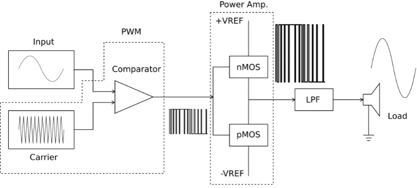
A Class-D amplifier is an electronic system where the amplification devices are, at any par-ticular moment, in fully on or off states. The basic aim of a Class-D operation is to create a train of pulses that is an encoded representation of the input. This is known as Pulse-Width Modulation, where when the pulses are averaged, original data information can be obtained [3]. Operation of a Class - D system can be visualized as shown in Figure 2.2. The system consists of a PWM that encodes incoming signals to two specified levels (usu-ally (-1,1)), by comparing instantaneous levels of the modulating carrier signal and the input signal, at the carrier’s sampling rate. The resulting output signal of the PWM is then a rectan-gular pulse train with instantaneous amplitudes being either of the two specified levels. The pulse train, when driving the amplification devices (power amplifier), produces an amplified version of the PWM output pulse train. This amplified pulse train is used to drive a low pass RLC filter (LPF) to produce an analog equivalent of the input signal.
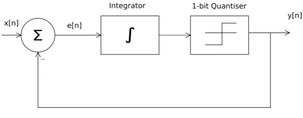
A digital Class - D amplifier controller is a digital control system that provides in - band noise reduction for a pulse width modulator amplifier. The control system is realized by enclosing the pulse width modulator in a negative feedback loop with a filter structure (loop filter) that is responsible for passing in - band frequency components of the input signal and moving the quantization noise from the PWM out of the bandwidth. A general structure of the controller is shown in Figure 2.3.
Figure 2.3: Basic digital Class - D amplifier controller
Vavg =Vh∗K+Vl∗(1−K) (2.1) where K is the duty cycle, ratio of ON time and period of the carrier.
As an example, calculation of the mean value of a 50% duty cycle, where both ON and OFF states are present for exactly the same amount of time, with a signal going from +1V to -1V is performed as follows
Vavg = 1∗0.5 + (−1)∗0.5 = 0V (2.2) The output of a Class-D amplifier in the absence of input is thus a square signal switching from the positive to the negative rail voltages, with 50% duty cycle. If the input is nearly at the maximum, for example 90%, then
Vavg = 1∗0.90 + (−1)∗0.10 = 0.8V (2.3)
Pulse-Width Modulation
Pulse - Width Modulation is a method of representing information in the form of a pulse train based on the input’s instantaneous amplitude. It is seen as a form of encoding the signal’s value in the form of pulses with varying widths. The interpretation of original input value from averaging of pulses is explained in the preceding section. Here, the internal workings of the modulator are presented.
2.3. PULSEWIDTHMODULATIONAMPLIFIER 13
the modulated output depends on the type of the sampling used.
The carrier frequency is to be at least twice the maximum frequency of the input, to satisfy the Nyquist criterion. In practice, however, the carrier frequency is chosen about 10 times the maximum frequency of the input signal bandwidth.
fcarr ≥10∗fmax (2.4)
PWM Sampling
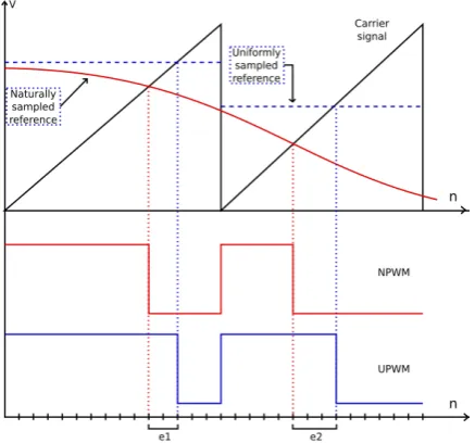
Pulse width modulation sampling is a term representing the kind of sampled modulation that takes place in a pulse width modulator in presence of a sampled input signal. In other words, a type of PWM sampling that depends on how an input reference signal that needs to be modulated is sampled in the first place. Accordingly, there are two types of PWM sam-pling, one that is based on continuous time and the other based on discrete time reference signals, known as Natural PWM and (NPWM) and Uniform PWM (UPWM) sampling. For analog systems, NPWM inherently occurs in PWM schemes, however for digital systems, UPWM is used as digital systems operate on discrete uniformly sampled quantized levels. NPWM fundamentally differs from UPWM, as illustrated in Figure 2.4.
In Figure 2.4, NPWM and UPWM schemes are presented, where nrefers to sampling
instants. In an NPWM sampling scheme, the reference signal (shown in red) is sampled at continuous time. In contrast, the reference signal for a UPWM scheme stays at a constant level (shown in blue), since this level is assumed to be a quantized value of the continuous time sampled equivalent. As a consequence, the carrier samples the continuous time ref-erence sample in NPWM earlier, compared to UPWM (in this example), when the carrier is a rising edge sawtooth waveform in this instance. When NPWM and UPWM waveforms are compared against each other, it becomes clear that there are errors present in UPWM scheme (e1 and e2), which contribute to distortion.
Figure 2.4: Natural and Uniform sampling for PWM
Preproccessing
In the previous section, it has been established that for a purely digital solution, UPWM scheme is realizable. The idea that UPWM operates on discrete samples of data drives a straightforward implementation of the PWM algorithm in the digital domain. However, UPWM suffers from errors as compared to NPWM. The challenge is therefore to design a UPWM scheme that satisfactorily comes close to matching NPWM.
To realize such a UPWM scheme, the incoming audio sample needs to undergo two stages of processing, namely oversampling and interpolation. Oversampling enables the incoming data to be sampled high enough to provide more number of samples than what is required by the Nyquist criteria. Interpolation is a ’reconstruction’ of the oversampled data and new data points are extracted from the interpolated signal, at the sample rate matching that of the oversampled data. The presence of a larger number of samples thus makes UPWM operation to be as close as possible to NPWM.
Converting sample rates is quite useful in DSP applications like communications, au-dio, speech processing and various other multi-rate systems. Sample rate conversions, upsampling and downsampling, exist to increase or decrease the sample rates of a signal respectively. In audio applications, oversampling is quite useful for increasing the frequency bandwidth of the signal, in order to employ Uniform PWM techniques, and eventually certain noise shaping techniques to improve the quality of audio.
2.3. PULSEWIDTHMODULATIONAMPLIFIER 15
Consider an input signalx(n). The upsampling algorithm is then given as
wm= (
x(m/K); m= 0,±K,±2K....
0; otherwise (2.5)
Translatingwm into the z - domain, we get
W(z) = ∞
X
m=−∞
w(m)z−m
= ∞
X
m=−∞
x(m)z−mK
=X(zK)
(2.6)
This method of increasing the sampling rate is, therefore, much straightforward. How-ever, there are fundamental frequency translated problems associated with it. The effective bandwidth now increases by upsampling, but replicas of the original signal now sit within the expanded bandwidth. This causes aliasing due to the replicas. It becomes evident when spectral content of the upsampled signal is compared to that of the original.
Interpolation in DSP sense is a process of smoothening the areas between two samples. It is a process of constructing a continuous function from discrete points of a signal, or more generally, it is a method of finding missing data within two consecutive samples of sampled data.
Interpolation is a much preferred application in cases where the data’s sample rate is to be changed. In the previous section, it has been shown that upsampling data by zero-padding causes replicas of original signal to be present in the expanded bandwidth. The objective is thus to remove those replicas by means of filtering. Filters constructed for this sole application are called interpolation filters.
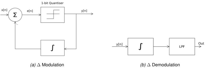
(a)∆Modulation (b)∆Demodulation
Figure 2.5:∆Modulation and demodulation chain
Noise Shaping
In previous sections, techniques like oversampling and interpolation of an input signal are used to increase the bandwidth of the audio band. The extended frequency band now en-ables further signal processing techniques that can be employed to reduce quantization noise by moving the noise outside the audio band, thus improving the quality of the output signal. The technique to perform this operation is known as noise shaping. With this method, it is possible to attain high - resolution audio while running at a moderate bit rate.
Noise shaping is seen as having a high pass characteristic, as it just relocates noise present in the system out of the audio band. This is an important step as the output low pass filter at the power stage filters out noise that has been moved out of the band of inter-est. The popular method to achieve noise shaping is to enclose the Pulse - Width modulator in a negative feedback loop [4]. The negative feedback enables error correction mechanism that is useful for reduction of noise. This structure is reminiscent of a Sigma - Delta (Σ∆)
modulator, where the system can operate on a high sample rate and the quantizer can be 1 - bit.
Digital noise shaping is primarily a Sigma - Delta (Σ∆) modulation by nature. TheΣ∆
modulator structure is derived from the established ∆ modulator - demodulator structure
shown in Figure 2.5 [5]. It consists of a quantizer, loop closed with an integrator in its feed-back path. The output of the modulator is then fed to a feed-forward integrator , which is then passed through the usual low pass filter to obtain the filtered output. Delta modulation is based on quantizing the change of the signal at each sample.
Derivation of aΣ∆ modulation from Figure 2.5 is straightforward. The ∆modulation
-demodulation process uses two integators. By the property of linearity in integration, the integrator before the output loop filter can be first moved before quantizer at the input of the summation point. After that, the feedback integrator and the integrator at the input can be merged to form a single integrator before the quantizer). The resultant structure is called a
2.4. CLASS- D AMPLIFIERCONTROLLER 17
Figure 2.6: 1 - bitΣ∆modulator
A loop filter is a structure often used in modulators that are required to have a high performance while maintaining a modest resolution. The loop filter replaces the integrator in aΣ∆modulator by extending its structure to a slightly more complex architecture. There
are many standard loop filter architectures for the purpose of noise shaping in a 1 - bit quantizer system. A choice can be made based on requirements like resource utilization or complexity, but for the major part, the design of loop the filter depends fundamentally on deriving transfer functions and extracting the filter specifications from the resulting transfer. Primary requirement for a loop filter is to have a high gain in the bandwidth to ensure a large reduction of error [6].
2.4 Class - D Amplifier Controller
In previous sections, a PWM amplifier was introduced. For this investigation, modeling and implementation of Class - D amplifier controller first starts with formalizing the implementa-tion in terms of a mathematical model, since funcimplementa-tional modeling is based on mathematical relations. While mathematical modeling is performed for system analysis, modeling and implementation of the system has a modular approach, wherein each behavior is treated individually. The system primarily consists of a PWM module, which has a comparator and quantizer functionality in - built, along with a loop filter module which is interfaced with PWM in a feedback loop. The translation from mathematical model to architectural model is then demonstrated by performing appropriate simulations on the architectural model.
2.4.1 Mathematical modeling
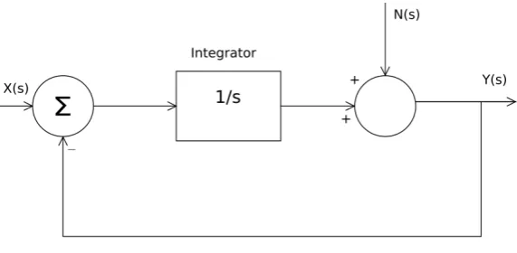
Figure 2.7: 1 - bitΣ∆modulator s - domain analysis
quantizer with some amount of quantization error reduction due to the inclusion of a filter in the loop, and the architecture is that of a 1 - bitΣ∆modulator, described in [5]. The loop filter
can be designed to be either a simple first order type or a complexnthorder type. To achieve a good performance, techniques are described in [7] and [8] which help in understanding the way to design a suitable transfer function behavior for higher order filters. In extension to the above mentioned methods, a loop filter architecture is derived after formulating a loop filter transfer function [9].
In Figure 2.6, a 1 - bitΣ∆modulator was presented. The 1 - bit quantizer is considered
as a noise source that provides the system with quantization noise. The system can then be re-visualized as shown in Figure 2.7, where the quantizer is now replaced with a summing point that adds a noise component N(s). At this stage, the noise shaping mechanism can
now be modeled in the s - domain as follows.
Y(s) = X(s)−Y(s) s Y(s)
X(s) = 1
s
1 +1s = 1 s+ 1
(2.7)
Y(s) =N(s)−Y(s) s Y(s)
N(s) = 1 1 +1s =
s s+ 1
(2.8)
The feedback loop integrates the difference between signal and noise, thereby low -passing the signal and high - -passing the noise. This means that the signal is not changed as long as it’s frequency is not above the filter’s cut - off limits. Equations mentioned above also illustrate the primary characteristic of noise shaping, in that the noise shaper acts as a high pass filter for noise and a low pass filter for signal. Noise shaping, and the modulator in extension, thus requires a wide bandwidth for it to operate, which is only possible by over-sampling the input signal to a high degree.
2.4. CLASS- D AMPLIFIERCONTROLLER 19
z domain as shown below. The integrator in s domain is an approximation of a continuous time model
Y(s) X(s) =
1 s
⇒y(t) =
Z t
0
x(t)dt
(2.9)
Realizing an integrator in discrete time is done by considering sampled time kT (T = time period, k = sample) and evaluating integrals over those limits. As a result,y(t)now becomes
y((k+ 1)T) =
Z (k+1)T
0 x(t)dt ⇒ Z kT 0 x(t)dt+
Z (k+1)T
kT
x(t)dt
⇒y(kT) +
Z (k+1)T
kT
x(t)dt
(2.10)
The discrete time approximation can now be translated into the z domain by the Euler integration approximation method. In this approximation, a change of output is calculated over the area underx(kT). This area can also be approximated as a rectangle of total area T x(k).
y((k+ 1)T) =y(kT) +T x(k)
y((k+ 1)T)−y(kT) =T x(k) (2.11)
After taking z transforms for above equations, the relation now becomes
zY(z)−Y(z) =T X(z) Y(z)
X(z) = T z−1 Y(z)
X(z) = T z−1 1−z−1 H(z) = T z
−1
1−z−1
(2.12)
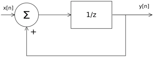
Equation 2.12 is the transfer function of a discrete time integrator, and it can be seen as a unit delay with a positive feedback, shown in Figure 2.8. For a single sampling stepT, the
transfer function simply becomesz−1/1−z−1. The Noise transfer function (NTF) for annth
order transfer is given by (from Equation 2.7)
N T F = 1 1 +1−z−z1−1 ⇒N T F = 1−z−1
N T F = (1−z−1)n F or nthorder
Figure 2.8: Integrator from unit delay
It is known that the higher the order of the noise shaper, the higher will be the SNR, and a modulator which includes annth order noise shaper in its implementation is known as an
nth order modulator. It then would mean that the order could be made sufficiently high, but
the straightforward solution is impractical as the size of the filter would be large.
H(z) is seen as a first - order loop filter in the system, but having a single order filter is
not sufficient to attain a high signal to noise ratio (SNR) of the system, since the gain pro-vided by a single pole filter (integrator) is not high enough. There are also issues like high frequency components folding back into the system, which are otherwise not filtered out by
H(z).
The open loop magnitude response of an integrator is a typical downward sloping re-sponse with a slope -20dB/decade. Addition of poles to the transfer function will increase
the rate of decay. However, when determining the response, it is desirable to have a flat slope at least in the band of interest. The slope can be flattened out by placing an additional complex pole pair and zero pair at higher frequencies [7] [8]. Addition of complex conjugate pairs of poles can be realized from the transfer function. Any filter with zeros b0, b1, b2..bm and polesa0, a1, a2..ancan be realized by the transfer function
Y(z) X(z) =
bmzm+bm−1zm−1+..+b1z+b0
anzn+an−1zn−1+..+a1z+a0 (2.14)
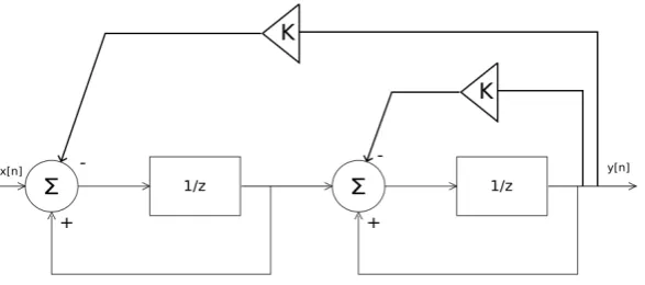
Assuming there are no zeros placed, the real poles translate to integrators (first order). Complex poles are then realized as a cascade of two first order sections with negative feed-back to each, with feedfeed-back gain(1−c1) + (1−c2), ifc1 andc2are the complex pole pairs.
The resultant realization is shown in Figure 2.9. This structure is termed as a resonator [9].
2.5. FUNCTIONALHARDWAREDESCRIPTIONS INHASKELL 21
Figure 2.9: Resonator structure
Yr(z)
Xr(z)
= 1
(z−1)((z−1) +K) +K
= 1
(z−1)2+ (z−1)K+K
= 1
z2+ (K−2)z+ 1
(2.15)
There exist a variety of filter transfers to implement in the modulator. For a higher order 1 - bit Σ∆ modulator, there are four typical structures of higher order loop filters that can
be implemented, varying in complexity and size. Since the focus is on implementing a fil-ter with resonator section, a Cascaded Integrators with Feed Forward summation (CIFF) is chosen. The CIFF structure is realized by interfacing an integrator with a resonator, in that order. This is due to the fact that an integrator can provide the highest dynamic range over the required bandwidth, and a resonator can keep the response of the passband flat. The filter is realized with the following transfer function, and architecture resembling Figure 2.10, which is a third order filter consisting of a first order section (integrator) and a second order section (resonator).
H(z) = 1 z−1 +
1
z2−2z+K+ 1+
1
(z2−2z+K+ 1)(K−1) (2.16)
2.5 Functional Hardware Descriptions in Haskell
2.5.1 Modeling in Haskell
Figure 2.10: 3rd order CIFF structure
Pulse - Width Modulator
The module definition for pulse - width modulator is defined in Listing 2.2. This module contains a triangular wave generator and a comparator that compares instantaneous values of input sample with instantaneous sample of the triangular wave generator’s output.
1 module Pwm
2 ( pwm -- main pwm function
3 , Slope
4 ) where
Listing 2.2: Module PWM definition
The module exports the functionpwmand data typeSlopeto the top level. The function pwmis responsible for generating a triangular wave, which is based an example presented
2.5. FUNCTIONALHARDWAREDESCRIPTIONS INHASKELL 23
1 data Slope = Up | Down
2
3 pwm :: (Num a,Fractional a,Floating a,Ord a) => (a,Slope) -> a -> ((a,Slope),a)
4 pwm (v,s) x = ((v’,s’),y)
5 where
6 v’ = case s of
7 Up -> v + 1/64
8 Down -> v - 1/64
9
10 s’ = case s of
11 Up | v’ < 1.0 -> Up
12 | otherwise -> Down
13 Down | v’ > -1.0 -> Down
14 | otherwise -> Up
15
16 y
17 | (x - v’) >= 0.0 = 1.0
18 | otherwise = -1.0
Listing 2.3: pwm definition
The type declaration forpwmis defined so as to make it polymorphic. Polymorphism in
Haskell comes from defining function types with type variables. IntriM, the type variable is
considered to bea. The type declaration then states thatacan be any number, as long as it
is of numerical typeN um, which is defined in the standard Haskell libraryP relude. The type
definition further defines variableato be asF ractional andF loating types, which support
fractional and floating point operations. The functiontriM also involves comparison of
ar-guments, hence the typeclassOrdis also used to declare variableato support>operation.
Mentioningawith the additional typesF loatingandF ractionalensure variableato be a
floating point number and that which can support fractional values and comparison as well. This means that effectively a is constrained to represent a floating point number, and the
process of putting such constraining a variable is done by declaring additional typeclasses.
After establishing the type of variablespwm operates on, the type definition ofpwm is
to be further extended with type behavior. pwm takes a tuple (v, s) containing a floating
point numbervand a state denoting a switching state (explained later) s, and a valuexas
arguments, and the evaluation is the resulting tuple((v0, s0), y), wherey is the present
out-put. The switching statesands0 (next switching state) is defined by a user-defined datatype Slope, which can at a time takeU porDown. Accordingly, the type definition for tuple
argu-ment(v, s)will be(a, Slope),nwill beaand finally((v0, s0), y)becomes((a, Slope), a).
In Listing 2.3, v is a present initial value, v0 is the next step of increment,sis the initial
which at any point of time can take up either of the fields U p orDown, thus signifying the
direction of traversal. The step size is an important parameter, as the step size effectively determines the frequency of the resulting wave, as described in Equation 2.17. Here, n
refers to number of steps of increment for 0 to maximum amplitude traversal or 0 to minimum amplitude traversal. Hence for a single cycle, there are4nnumber of traversal steps.
ftri=
fclk
4n (2.17)
The triangular wave is generated as follows. The function is initialized in a predefined start condition, in this case, value 0 and direction of increment as U p. Since the specified
incremental direction is U p, the next calculated output will be a positive increment of the
present value, with a fraction of step size. In this juncture, it is important to note that the fraction of the step size depends on the final peak amplitude of the required wave. For this research, the requirement is 2 V peak to peak, meaning the maximum traversals of the wave should be +1 and -1 V. Hence, increment step becomes1/n. For a peak valuek, the
incre-ment isk/n.
Along with the aforementioned process, pwmalso takes care of direction switching. It
constantly evaluates the next traversal direction by comparing the output value against the required peak values. If the present traversal is U p and the output is less than the peak,
the direction switch stays U p else it switches toDown. When the traversal is Down, the
present output is decremented with the same traversal step until it matches the minimum peak amplitude, and the switch turns toU pagain. In this way, a triangular wave is created.
In the introduction for PWM, it is mentioned that in practical applications, the frequency of the carrier should be high enough, about 10 times or more, than the highest frequency component in the bandwidth. For this PWM model, the simulations for triangular wave gen-eration are carried out by considering two values of nas 32 and 64, by providing an input
sine wave at 20 KHz, since it is the highest frequency considered in the audio bandwidth. The simulation results are shown in Figures 2.11a and 2.11b respectively. From the simula-tions, it can be seen that fornas 64, the triangular wave is nearly 10 times the frequency of
the input and forn as 32, the triangular wave is about 20 times. For the purpose of
imple-mentation,nas 64 is considered sufficient.
Second phase of the PWM module is comparison. This functionality is defined by the declaration forywhich compares the inputxand current triangular wave sample valuev0by
first subtracting them and comparing the resultant difference with 0. If the difference is≥0,
2.5. FUNCTIONALHARDWAREDESCRIPTIONS INHASKELL 25
(a)32 steps per rising/falling edge
[image:33.595.139.484.96.430.2](b)64 steps per rising/falling edge
Figure 2.11: Simulation results for n = 32 and n = 64
[image:33.595.118.512.497.728.2]1 y
2 | (x - v’) >= 0.0 = 1.0
3 | otherwise = -1.0
Listing 2.4: pwm definition
The functionpwmis simulated with an input with frequency 2KHz and a triangular wave
carrier with 64 steps per rising/falling edge (n), and the result is shown in Figure 2.12. It can
be seen that the result ofpwmfunction varies in widths corresponding to the duration of the
input staying high or low.
Loop Filter
Module definition of the loop filter is given in Listing 2.5. Similar to PWM, it exports function
lf ilterto the top level for system integration.
1 module Lfilter
2 (lfilter
3 )where
Listing 2.5: Lfilter module definition
Listing 2.6 shows the model of thelf ilterfunction. The loop filter architecture is a
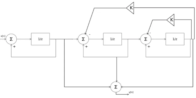
mod-ified version of the one presented in Figure 2.10, where intermediary gains are inserted to ensure loop stability, resulting in a structure shown in Figure 2.13. Functionlf ilter models
mathematical operations that are essential to the architecture in Haskell definitions. Similar-ities can be observed between Figure 2.10 andlf ilter, which is explained below.
In Section 2.3, the theory of loop filter is presented wherein the loop filter that is con-sidered for this case consisted of a first order integrator cascaded with a resonator, and the transfer functions of both sections were derived in the z domain. For realizing the lf ilter
model from the mathematical descriptions of the loop filter stages, the transfer functions of each stage is first converted into discrete time domain. Equation 2.18 shows the discrete time model of the first order integrator stage, and Equation 2.19 shows the discrete time model of the resonator stage. In Equation 2.18,y1[n]andx1[n]are present state output and
input of the first order integrator respectively, andy1[n+ 1]is the next state output.
Y1(z) X1(z) =
1 z−1 ⇒zY1(z)−Y1(z) =X1(z)
⇒y1[n+ 1] =y1[n] +x1[n]
2.5. FUNCTIONALHARDWAREDESCRIPTIONS INHASKELL 27
Figure 2.13: Loop filter implementation
Similarly in Equation 2.19, the discrete time equation for resonator is derived by deriving the individual transfer functions of each integrator in the structure, thus resulting iny2[n+ 1]and y3[n+ 1]next state outputs for the second and the third integrator respectively.
y2[n+ 1] =y2[n] +x2[n]−a23y3[n]
y3[n+ 1] =y3[n] +x3[n]−a33y3[n]
(2.19)
Thus, the output of the loop filter y[n+ 1] is given in Equation 2.20. The equation
de-scribes the mathematical expression of a third order CIFF loop filter in discrete time domain.
y[n+ 1] =y1[n+ 1] +y2[n+ 1] +y3[n+ 1]
y[n+ 1] =x1[n] +x2[n] +x3[n] +y1[n] +y2[n] +y3[n]−a23y3[n]−a33y3[n] (2.20)
After including feed-forward gain multiplying factors a21 and a32, the equation now
be-comes as shown in Equation 2.21. Also, since the values x2[n]and x3[n]are originating
directly fromy1[n]andy2[n]respectively, they can be substituted withy1[n]andy2[n].
y[n+ 1] = 1∗x1[n] +a21∗y1[n] +a32∗y2[n]
+y1[n] +y2[n] +y3[n]−0∗y3[n]−a23∗y3[n]−a33∗y3[n]
⇒y[n+ 1] =g1 +g2 +g3
W here, g1 = 1∗x1[n] +y1[n] + 0∗y3[n]
g2 =a21∗y1[n] +y2[n] + (−a23)∗y3[n]
g3 =a32∗y2[n] +y3[n] + (−a33)∗y3[n]
(2.21)
A correspondence is now made between the discrete time formulation derived in Equa-tion 2.21, and the Haskell model oflf ilter, as shown in Figure 2.14. To model this equation,
Figure 2.14: lfilter model in Haskell
operations on the elements of those lists. For example, the feed-forward gain factors are defined asffcoef, which is a list containing values (1,a21,a32) and the feedback gain factors
are defined by the list fbcoef containing the values (0,a23,a33). The present outputs can
be represented by a lists of 3 elements that models the present states. The operations in
the above defined groups g1,g2 and g3 are carried out by three different functions, which
are present in the Haskell P relude library. To multiply the feed-forward gain factors, the zipW ith(∗)function is used to multiplyffcoef with a listxscomposed of(x1[n], y1[n], y2[n])
and the feedback gain factorsfbcoef are multiplied withy3[n]by using the map(∗(last s))
function. Results of gain factor multiplications are all lists, and they are added with present statessto essentially form a listvscontaining(g1, g2, g3)of Equation 2.21. Finally, the
out-put is obtained by adding the elements(g1, g2, g3)by using thef oldl(+)function, that adds
all the elements in a list.
1 lfilter :: (Num a,Floating a) => [a] -> (a,a) -> ([a],a)
2 lfilter s (x1,x2) = (s’,y)
3 where
4 (a21,a23,a32,a33) = ((2.368164*(10**(-2))),(-1.617432*(10**(-3))),
5 (1.208496*(10**(-2))),(-1.955032*(10**(-5))))
6
7 fbcoef = [0,a23,a33]
8 ffcoef = [1,a21,a32]
9
10 x = x1 + x2
2.6. CONCLUSIONS 29
12 ls = zipWith (+) us s
13 xs = zipWith (*) ([x] ++ init s) ffcoef
14 vs = zipWith (+) xs ls
15
16 s’ = vs
17 y = foldl (+) 0 s
Listing 2.6: lfilter function definition
Closed loop system
Listing 2.7 details the Haskell model for the Class - D amplifier controller, which is visualized in Figure 2.15. In this function, statesis a list of four values, with the first three values
rep-resenting states of the loop filter, while the last value represents a state for the entire closed loop system to enable feedback modeling.
1 cdAmp :: (Floating a, Ord a,Enum a) => [a] -> a -> ([a],a)
2 cdAmp s x = (s’,y)
3 where
4 s1 = init s
5 s2 = tail s
6
7 (s1’,u) = lfilter s1 ((-1) * last s) x
8 y = snd $ pwm (0,Up) u
9
10 s2’ = [y]
11
12 s’ = s1’ ++ s2’
Listing 2.7: Closed loop model CDAmp
2.6 Conclusions
This chapter explained the introductory theory about a PWM amplifier and associated fun-damentals essential to it. Further explanation was given about a 1 - bitΣ∆ modulator. The
most important section of aΣ∆modulation scheme is the loop filter, and the choice of a
suit-able topology to obtain required characteristics is shown. For this research, a CIFF structure was chosen due to its simplicity.
Figure 2.15: System model in Haskell
Chapter 3
Implementation in C
λ
aSH
3.1 Introduction
In Chapter 2, the concept of describing digital hardware in functional languages was pre-sented with examples of two existing languages that have been used for a long time. The languages mentioned are called embedded domain specific languages, or EDSLs, which contain pre-defined special functions to simulate a hardware specification. The language CλaSH is a sub-set of Haskell, that borrows syntax and semantics from Haskell. This
means that the compiler environment is also the same. Aside from type conversions and rewriting, a CλaSH specification is the same as the Haskell model, and the simulations can
be performed by a native Haskell compiler [11]. In addition to that, CλaSH also supports
polymorphism and higher order application of functions directly, since it is based on Haskell.
The retyping is done in order to properly convert a Haskell base model into a CλaSH
implementation. There are two major type conversions to be done. This is necessary since some dynamic structures like lists and trees in Haskell are not directly realizable in hard-ware implementation [11]. To overcome this, lists in Haskell are converted toV ectors, which
have a defined size and are recognized by CλaSH. Another retyping is done for
represent-ing integers and floatrepresent-ing point values. Currently, CλaSH supports representation of fixed
point numbers in both Signed and Unsigned forms. Conversion of floating point types to fixed point types can be made by retyping the function type with appropriate representation formats.
In the beginning of this research, a core reference model of Class - D amplifier was made in Haskell. The following sections describe retyping of the Haskell code to convert it into a CλaSH specification.
3.1.1 Data types and conversions
In Haskell model, a global type that represented values in all phases of operations was floating point. For most designs and even actual DSP processes, floating point arithmetic is preferred over fixed - point, due to its superior precision. However, implementing floating point on hardware is resource intensive, specially in areas where operations are performed with word lengths exceeding 24 bits wide. A trade-off is thus usually considered by selecting fixed - point representation for values.
There are issues working with fixed - point representation. First, there is the issue of integer overflow, which happens when the number of bits used in the format are not enough to represent extreme values. Secondly, care should be taken in selecting a fixed - point format when employing signed values. Fortunately, CλaSH compiler can be used to inspect
maximum and minimum bounds of representation with full precision, after which one can select a suitable format.
In this CλaSH implementation, a signed fixed - point format Q6.18 was selected. The
decision was made by observing the impulse response of the loop filter, maximum and minimum values of coefficients and the resolution of triangular wave carrier. The impulse re-sponse is presented in Figure 3.1, where the maximum amplitude of the rere-sponse is around 31. Also, the triangular wave (carrier) is implemented to have peak values as -1 and +1. Thus, the format to accommodate the value 31 in signed fixed point needs to contain 6 bits integer bits, since the minimum and maximum bounds for 6 integer bits are (-32,31), whereas for 5 integer bits are (-16,15), and the limits were found by using the minBound
and maxBound functions available in the CLaSH.F ixed library. The number of fractional
bits can now be anything from 0 to 26. To get a better precision, Q2.26 can be used to utilize a full 32 - bit length, however, keeping in mind standard audio format is 24 bits wide, Q6.18 was chosen instead.
Pulse Width Modulator
Listing 3.1 shows CλaSH implementation of pwm. Similar to Haskell model, the primary
function is pwm, and step size is defined with value 0.015625 (requirement 1/64 per step
per half edge traversal). The datatype Slope is also retained to switch between U p and Down. As discussed in previous section, a typeSampleis defined as signed fixed point type
in Q6.18 format. Additionally, -1 and +1, being floating point values, need to be defined as
Sampleas well. For this conversion,f Litfunction available in CλaSH Prelude library [12] is
3.1. INTRODUCTION 33
Figure 3.1: Loop filter impulse response
1 type Sample = SFixed 6 18
2
3 n = $$(fLit 0.015625) :: Sample
4 llim = $$(fLit (-1.0)) :: Sample
5 ulim = $$(fLit 1.0) :: Sample
6
7 data Slope = Up | Down
8
9 pwm :: (Sample,Slope)
10 -> Sample
11 -> ((Sample,Slope),Sample)
12 pwm (v,s) x = ((v’,s’),y)
13 where
14 v’ = case s of 15 Up -> v + n
16 Down -> v - n
17
18 s’ = case s of
19 Up | v’ < ulim -> Up
20 | otherwise -> Down
21 Down | v’ > llim -> Down
22 | otherwise -> Up
23
24 y
25 | (x - v’) >= 0 = ulim
26 | otherwise = llim
Loop Filter
Conversion from lists used in Haskell code to Vectors is perhaps best shown in Listing 3.2, which shows the CλaSH implementation of loop filter. For modeling lists as vectors, a new
type SampleV ec3 is declared, which is a vector of size 3, and each value of that vector is
signed fixed - point Q6.18 Sample. Another vector operation to note is vector initialization.
In CλaSH, it is done with a:>operator, which appends a value left to it to the value on the
right. In this implementation for example, vectorffcoef is initialized with valuesa23anda33,
In this way, listffcoef of Haskell model is modeled in CλaSH, and similarlyfbcoef as well.
CλaSH implementation oflf ilterdiffers from its Haskell counterpart in some ways. While
most of the algorithm remains same, multiplication (in functionf pmult) is realized in CλaSH
implementation by using the function‘times‘after which the result is resized to the required
datatype using‘resizeF‘, which is a resizing function for fixed point numbers. Both‘times‘
and‘resizeF‘functions are available in ’Prelude.Fixed’ library of CλaSH.
1 type Sample = SFixed 6 18
2 type SampleVect3 = Vec 3 Sample
3
4 a33 = -1.955032e-5 :: Sample
5 a23 = -1.617432e-3 :: Sample
6 a21 = 2.368164e-2 :: Sample
7 a32 = 1.208496e-2 :: Sample
8
9 fbcoef = 0 :> a23 :> a33 :> Nil
10 ffcoef = 1 :> a21 :> a32 :> Nil
11
12 fpmult :: Sample -> Sample -> Sample
13 fpmult a b = c
14 where
15 c = resizeF (a ‘times‘ b) :: Sample
16
17 lfilter :: SampleVect3 -> (Sample,Sample) -> (SampleVect3, Sample)
18 lfilter s (x1,x2) = (s’, y)
19 where
20 x = resizeF (x1 ‘plus‘ x2) :: Sample
21 us = map (fpmult (last s)) fbcoef
22 ls = zipWith (‘plus‘) us s
23 xs = zipWith (fpmult) ([x] ++ init s) ffcoef
24 vs = zipWith (‘plus‘) xs ls
25
26 s’ = vs
27 y = foldl (‘plus‘]) 0 s
3.1. INTRODUCTION 35
3.1.2 Closed loop system
Listing 3.3 shows the CλaSH implementation of Class - D amplifier. The typeCDSampleis
also Q6.18 since the type is propagated to other modules. Afterwards, a functionbundleis
used, which takes two values of typeSignaland merges them into a tuple of the typeSignal
that is synchronous with system clock. Top entity annotations are defined for creating an RTL code that acts as a wrapper for actualtopEntity declaration.
1 {-# ANN topEntity
2 (defTop
3 { t_name = "cdamparchM"
4 , t_inputs = ["I_in"]
5 , t_outputs = ["O_out"]
6 }) #-}
7
8 type CDSample = SFixed 6 18
9 type CDSampleVect4 = Vec 4 CDSample
10
11 cdAmp :: CDSampleVect4 -> CDSample -> (CDSampleVect4,CDSample)
12 cdAmp s x = (s’,y)
13 where
14 s1 = init s
15 s2 = last s
16
17 (s1’,u) = lfilter s1 (x,(last s))
18 y = snd $ pwm (0,Up) u
19
20 s2’ = y :> Nil
21 s’ = s1’ ++ s2’
22
23 cdamparchM = mealy cdAmp (repeat 0)
24
25 topEntity :: Signal CDSample -> Signal CDSample
26 topEntity = cdamparchM
Listing 3.3: CλaSH closed loop model CDAmp
In Haskell models, a notion of state was modeled in thepwmandlf ilterfunctions.
How-ever, in CλaSH, sequential designs which contain a notion of state need to be declared with
an initial state. This is done by using themealyfunction for thecdAmp function. In CλaSH,
the function type ofmealyis described as shown in Listing 3.4 [12]. mealytakes a function
having the signature of the types→ i→ (s0, o), where sis present state, iis input and the
tuple (s0, o) is the next state and output. A second argument is input iof the type Signal,
which is used in functions that are translated to top level entities. The output is denoted by
can be converted to mealy state machine function, given bycdamparchM.
1 mealy :: (s -> i -> (s, o))
2 -> Signal i
3 -> Signal o
Listing 3.4: CλaSH mealy function type description
3.2 Conclusions
In this chapter, modeling and implementation of a basic Class - D amplifier has been carried out. In Haskell, modeling was performed in a modular fashion to accentuate the structural design aspect of design in a functional semantic environment, and to also to make the model easier to read. Implementation in CλaSH was done by transforming the Haskell code with
modifications, without sacrificing the original approach.
In the next chapter, results of Haskell and CλaSH models are shown and compared
against each other. As an additional exercise, both models are also compared against a Simulink model. The reason behind this exercise is to show how in a basic sense Haskell itself can be used to model digital systems in the first place, and then how CλaSH
Chapter 4
Results and Comparisons
In the previous chapter, modeling and implementation of a Class - D amplifier controller in Haskell and CλaSH were discussed respectively. In this chapter, simulation results of both
models are presented and compared.
For both Haskell and CλaSH simulations, a simulation flow was built, as shown in Figure
4.1. In case of Haskell simulations, primary inputs were given to the top level function, and results were written to a text file by using IO functionality. The text file was transformed to a comma - separated values (.csv) file from which values were extracted by a MATLAB script (seeAppendix B) that calculates Power Spectrum Density (PSD) and performance figures [13]. CλaSH simulation differed from Haskell in that the input was defined in top level
CλaSH code, usingsimulatefunction provided in the CλaSH library.
After performing the required simulations on Haskell and CλaSH models, comparisons
are made on an existing Simulink model of the system. This model was built to represent the intended system as a basic reference. It is speculative at this point as to whether the Haskell model itself could represent as reference, however, since the CλaSH implementation
[image:45.595.166.458.578.739.2]was done by translating Haskell code itself, the Simulink model was also brought into this
Figure 4.1: Simulation Environment flow
perspective to illustrate how the Haskell model agrees to its implementation in the first place. The Simulink top level is shown in Figure 4.2. Here, the subsystem blocks are connected as per the Class - D amplifier controller architecture.
The simulation results of the Simulink model, the Haskell model and the CλaSH
imple-mentation include two points of comparison. The first subject of comparison is the intended behavior of the system. It has been discussed in Chapter 2 that the Class - D amplifier controller system should exhibit a noise shaping behavior. This means that the noise, which is the quantization noise occuring around the frequency of the carrier signal and its integer multiples, should be moved outside the band of interest, which is from 0 Hz to 20 KHz, and the behavior is viewed in the form of power spectral density (PSD) plots. In the obtained PSD plots, the points of interest are the central frequency gain occuring at the frequency of the applied input signal, and the quantization noise out of the band exhibiting a high pass behavior. The second subject of comparison is done from the obtained signal to noise ratio (SNR) values from the system’s response. However, most of the interest is on evaluating the noise shaping behavior of the system.
4.1 Haskell Simulation
Simulation is performed by passing a list containing sampled values of a sine function. The sine wave has a frequency of 6 kHz, with sampling frequency 49.152 MHz. This frequency was chosen keeping in view that this frequency was required to generate a triangular carrier of 192 kHz and that which contains 256 steps in one cycle, since the PWM sampling for one cycle contains 256*192 K = 49152 K samples. Also, the amplitude of the input was kept 0.5.
Figure 4.3 shows the pulse spectrum density (PSD) plots of Simulink model and Haskell model output. It clearly shows the expected noise shaping that happens out of the audio band. The first carrier frequency component occurs at 192 kHz and its copies are at integral multiples of its base frequency.
4.2 C
λ
aSH Simulation
The CλaSH simulation follows the Haskell simulation in terms of parameters, whereas the
method is different. As shown in Listing 4.1, the keywordsimulateis used which evaluates
the function cdAmp with the input list inpdata. Just like with other values in the code, the
input should also follow the same format, which is signed fixed - point Q6.18.
Figure 4.4 shows the PSD plots of Simulink and CλaSH simulation results. Here too,
4.2. CλASH SIMULATION 39
(a)Top level Simulink model
(b)Pulse Width Modulator
(c)Triangular wave generator (carrier)
[image:47.595.172.447.118.744.2](d)Loop filter
(a)Simulink Simulation
[image:48.595.73.498.170.387.2](b)Haskell Simulation
4.2. CλASH SIMULATION 41
(a)Simulink Simulation
[image:49.595.101.530.168.392.2](b)CλaSH Simulation
1 f6 = 5812.5
2 w6 t = 0.5*(sin(2*pi*f6*t))
3 st = [0,(1/(1024*48000))..1]
4
5 inpdata = L.map fLitR (L.map w6 st) :: [CDSample]
6
7 res = simulate cdAmp inpdata
Listing 4.1: CλaSH simulation of Class - D amplifier
The MATLAB script also calculated signal parameters like Signal - to - Noise Ratio (SNR) and Total Harmonic Distortion plus Noise (THDN). Table 4.1 gives an overview of the calcu-lated values for both Haskell and CλaSH simulations.
[image:50.595.122.306.313.377.2]Simulation SNR (dB) THDN (dB) Simulink 109.06 -106.14 Haskell 109.75 -104.13 CλaSH 110.88 -103.19
Table 4.1: Simulation comparisons of Simulink, Haskell and CλaSH
From the values obtained, it is clearly seen that the Signal to noise ratio is well above 100 dB for all three models, which is usually a characteristic of a 1 - bit Class - D modulator. The difference of about 1 dB between the Haskell model and the CλaSH implementation
can be because of the differences between floating point and fixed point formats.
4.3 Synthesis
Any RTL code that needs to be realized as physical hardware, should be synthesizable. In the beginning of this research CλaSH was introduced along with a feature that enables it to
generate VHDL code that is synthesizable. When developing a design in bare VHDL, one must follow certain coding guidelines in order to make the design synthesizable. CλaSH
generated code however is readily synthesizable on to hardware.
The generated VHDL top entity code is an entity with port descriptions mentioned in the top level AN N annotations. In addition, CλaSH also generates other RTL files on which
the top level design description depends. To see how the design is synthesized, the gen-erated top entitycdAmp.vhdl is synthesized by Quartus with target device set to Cyclone II
EP2C20F484C7. The synthesis results are shown in Figure 4.5.
The RTL view of cdAmp is also presented in Figure 4.6. In this RTL view, the block cdamp lfilter is the loop filter and the block cdamp pwmis the PWM block. The system’s
4.4. CONCLUSIONS 43
Figure 4.5: Synthesis result of cdAmp.vhdl
Figure 4.6: RTL view of cdAmp.vhdl
denoted asresult.tup2 1 sel1[23..0] which at top level is connected toy[23..0]and it follows
the same datatype as the input.
4.4 Conclusions
In this chapter, simulations were first performed on a Haskell model and a CλaSH
imple-mentation of a Class - D amplifier controller. Since the CλaSH implementation was derived
from Haskell, the Haskell model’s correctness was first established by comparing its simula-tion results with a Simulink model. The simulasimula-tion verificasimula-tion was performed on two fronts, obtaining the PSD response and a quantitative comparison of obtained performance figures. Haskell model’s results closely resembled that of Simulink variant.
Simulation results obtained from the CλaSH model reflected the resemblance with it’s
Haskell counterpart. The results compared in a similar way with Simulink results confirmed the similarities with the CλaSH implementation and the Haskell model. Furthermore, the
performance figures recorded by both CλaSH and Haskell were comparable and very less
[image:51.595.110.519.280.354.2]Synthesis was performed on the top level entity VHDL description that was generated by the CλaSH compiler. The results show that the design is indeed synthesizable, with the