University of Warwick institutional repository: http://go.warwick.ac.uk/wrap
This paper is made available online in accordance with publisher policies. Please scroll down to view the document itself. Please refer to the repository record for this item and our policy information available from the repository home page for further information.
To see the final version of this paper please visit the publisher’s website. Access to the published version may require a subscription.
Author(s): Lee, Wonjung, McDougall, D. and Stuart, A. M. Article Title: Kalman filtering and smoothing for linear wave equations with model error
Year of publication: 2011
Link to published article:
http://dx.doi.org/10.1088/0266-5611/27/9/095008
arXiv:1101.5096v2 [math.PR] 12 Jul 2011
equations with model error
Wonjung Lee1,2, D. McDougall1 and A.M. Stuart1 1Mathematics Institute, University of Warwick, Coventry, CV4 7AL, UK 2Mathematical Institute, University of Oxford, Oxford, OX1 3LB, UK
E-mail:
[email protected] [email protected]
[email protected] http://www.warwick.ac.uk/∼masdr/
Abstract. Filtering is a widely used methodology for the incorporation of observed data into time-evolving systems. It provides an online approach to state estimation inverse problems when data is acquired sequentially. The Kalman filter plays a central role in many applications because it is exact for linear systems subject to Gaussian noise, and because it forms the basis for many approximate filters which are used in high dimensional systems. The aim of this paper is to study the effect of model error on the Kalman filter, in the context of linear wave propagation problems. A consistency result is proved when no model error is present, showing recovery of the true signal in the large data limit. This result, however, is not robust: it is also proved that arbitrarily small model error can lead to inconsistent recovery of the signal in the large data limit. If the model error is in the form of a constant shift to the velocity, the filtering and smoothing distributions only recover a partial Fourier expansion, a phenomenon related to aliasing. On the other hand, for a class of wave velocity model errors which are time-dependent, it is possible to recover the filtering distribution exactly, but not the smoothing distribution. Numerical results are presented which corroborate the theory, and also to propose a computational approach which overcomes the inconsistency in the presence of model error, by relaxing the model.
Submitted to: Inverse Problems
1. Introduction
the effect of model error – the mismatch between model used to filter and the source of the data itself. In this paper we undertake a study of the effect of model error on the Kalman filter in the context of linear wave problems.
Section 2 is devoted to describing the linear wave problem of interest, and deriving the Kalman filter for it. The iterative formulae for the mean and covariance are solved and the equivalence (as measures) of the filtering distribution at different times is studied. In section 3 we study consistency of the filter, examining its behaviour in the large time limit as more and more observations are accumulated, at points which are equally spaced in time. It is shown that, in the absence of model error, the filtering distribution on the current state converges to a Dirac measure on the truth. However, for the linear advection equation, it is also shown that arbitrarily small model error, in the form of a shift to the wave velocity, destroys this property: the filtering distribution converges to a Dirac measure, but it is not centred on the truth. Thus the order of two operations, namely the successive incorporation of data and the limit of vanishing model error, cannot be switched; this means, practically, that small model error can induce order one errors in filters, even in the presence of large amounts of data. All of the results in section 3 apply to the smoothing distribution on the initial condition, as well as the filtering distribution on the current state. Section 4 concerns non-autonomous systems, and the effect of model error. We study the linear advection equation in two dimensions with time-varying wave velocity. Two forms of model error are studied: an error in the wave velocity which is integrable in time, and a white noise error. In the first case it is shown that the filtering distribution converges to a Dirac measure on the truth, whilst the smoothing distribution converges to a Dirac measure which is in error, i.e., not centred on the truth. In the second, white noise, case both the filter and smoother converge to a Dirac measure which is in error. In section 5 we present numerical results which illustrate the theoretical results. We also describe a numerical approach which overcomes the effect of model error by relaxing the model to allow the wave velocity to be learnt from the data.
filters will not work well in high dimensions [14, 15, 16]. As a consequence a great deal of research activity is aimed at the development of various approximation schemes within the filtering context; see [17, 18, 19, 20, 21, 22] for example. The subject of consistency of Bayesian estimators for noisily observed systems, which forms the core of our theoretical work in this paper, is an active area of research. In the infinite dimensional setting, much of this work is concerned with linear Gaussian systems, as we are here, but is primarily aimed at the perfect model scenario [23, 24, 25]. The issue of model error arising from spatial discretization, when filtering linear PDEs, is studied in [26]. The idea of relaxing the model and learning parameters in order to obtain a better fit to the data, considered in our numerical studies, is widely used in filtering (see the chapter by K¨unsch in [2], and the paper [27] for an application in data assimilation).
2. Kalman Filter on Function Space
2.1. Statistical model for discrete observations
The test model, which we propose here, is a class of PDEs
∂tv+Lv = 0, ∀(x, t)∈T2×(0,∞) (1)
on a two dimensional torus. Here L is an anti-Hermitian operator satisfying L∗ = −L
where L∗ is the adjoint in L2(T2). Equation (1) describes a prototypical linear wave
system and the advection equation with velocity c is the simplest example:
∂tv+c· ∇v = 0, ∀(x, t)∈T2×(0,∞). (2)
The state estimation problem for Equation (1) requires to find the ‘best’ estimate of the solutionv(t) (shorthand forv(·, t)) given a random initial conditionv0 and a set of noisy
observations, called data. Suppose the data is collected at discrete timestn =n∆t, then
we assume that the entire vn = v(tn) solution on the torus is observed with additive
noiseηnat timetn, and further that theηn are independent for differentn. Realizations
of the noise ηn are L2(T2)-valued random fields and the observationsyn are given by
yn =vn+ηn =e−tnLv0+ηn, ∀x∈T2. (3)
Here e−tL denotes the forward solution operator for (1) through t time units. Let
YN = {y1, . . . , yN} be the collection of data up to time tN, then we are interested in
finding the conditional distribution P(vn|YN) on the Hilbert space L2(T2). If n = N,
this is called the filtering problem, ifn < N it is the smoothing problem and forn > N, the prediction problem. We here emphasize that all of the problems are equivalent for our deterministic system in that any one measure defines the other simply by a push forward under the linear map defined by Equation (1).
In general calculation of the filtering distribution P(vn|Yn) is computationally
challenging when the state space forvnis large, as it is here. A key idea is to estimate the
signalvnthrough sequential updates consisting of a two-step process: prediction by time
followed by an analysis step which corrects the probability distribution on the basis of the statistical input of noisy observations of the system using Bayes rule:
P(vn+1|Yn+1)
P(vn+1|Yn) ∝
P(yn+1|vn+1). (4)
This relationship exploits the assumed independence of the observational noises ηn
for different n. In our case, where the signal vn is a function, this identity should
be interpreted as providing the Radon-Nikodym derivative (density) of the measure
P(dvn+1|Yn+1) with respect to P(dvn+1|Yn) [28].
In general implementation of this scheme is non-trivial as it requires approximation of the probability distributions at each step indexed by n. In the case of infinite dimensional dynamics this may be particularly challenging. However, for linear dynamical systems such as (1), together with linear observations (3) subject to Gaussian observation noise ηn this may be achieved by use of the Kalman filter [3]. Our
work in this paper begins with Theorem 2.1, which is a straightforward extension of the traditional Kalman filter theory in finite dimension to measures on an infinite dimensional function space. For reference, basic results concerning Gaussian measures required for this paper are gathered in Appendix A.
Theorem 2.1. Let v0 be distributed according to a Gaussian measure µ0 =N (m0,C0)
on L2(T2) and let {η
n}n∈N be i.i.d. draws from the L2(T2)-valued Gaussian measure
N(0,Γ). Assume further that v0 and {ηn}n∈N are independent of one another, and that
C0 and Γ are strictly positive. Then the conditional distribution P(vn|Yn) ≡ µn is a
Gaussian N(mn,Cn) with mean and covariance satisfying the recurrence relations
mn+1 =e−∆tLmn
−e−∆tLCne−∆tL∗ Γ +e−∆tLCne−∆tL∗−1
e−∆tLmn−yn+1
,(5a)
Cn+1 = e−∆tLCne−∆tL∗
−e−∆tLCne−∆tL∗ Γ +e−∆tLCne−∆tL∗−1
e−∆tLCne−∆tL∗, (5b) where m0 =m
0, C0 =C0.
Proof. Letmn|N =E(vn|YN) andCn|N =E
(vn−mn|N)(vn−mn|N)∗
denote the mean and covariance operator of P(vn|YN) so that mn =mn|n, Cn =Cn|n. Now the prediction
step reads
mn+1|n=E(e−∆tLvn|Yn) =e−∆tLmn|n,
Cn+1|n =E
e−∆tL(vn−mn|n)(vn−mn|n)∗e−∆tL ∗
=e−∆tLCn|ne−∆tL ∗
. (6)
To get the analysis step, choose x1 =vn+1|Yn and x2 =yn+1|Yn then (x1, x2) is jointly
Gaussian with mean (mn+1|n, mn+1|n) and each components of the covariance operator
for (x1, x2) are given by
C11 =E
(x1 −mn+1|n)(x1−mn+1|n)∗
=Cn+1|n,
C22 =E
(x2 −mn+1|n)(x2−mn+1|n)∗
C12 =E
(x1 −mn+1|n)(x2−mn+1|n)∗
=Cn+1|n=C21.
Using Lemma A.2 we obtain
mn+1|n+1 =mn+1|n− Cn+1|n Γ +Cn+1|n
−1
mn+1|n−yn+1
,
Cn+1|n+1 =Cn+1|n− Cn+1|n Γ +Cn+1|n
−1
Cn+1|n. (7)
Combining Equations (6) and (7) yields Equation (5).
Note that µn, the distribution of v0|Yn, is also Gaussian and we denote its mean
and covariance by mn and Cn respectively. The measure µn is the image of µn under
the linear transformation etnL. Thus we have m
n =etnLmn and Cn =etnLCnetnL ∗
. In this paper we study a wave propagation problem for which L is anti-Hermitian. Furthermore we assume that both C0 and Γ commute with L. Then the formulae (5) simplify to give
mn+1 =e−∆tLmn− Cn(Γ +Cn)−1 e−∆tLmn−yn+1
, (8a)
Cn+1 =Cn− Cn(Γ +Cn)−1
Cn. (8b)
The following gives explicit expressions for (mn,Cn) and (mn,Cn), based on the
Equations (8).
Corollary 2.2. Suppose that C0 and Γ commute with the anti-Hermitian operator L, then the means and covariance operators of µn and µn are given by
mn= nI + ΓC0−1
−1 "
ΓC0−1m0+
n−1
X
l=0
etl+1Ly l+1
#
, (9a)
Cn = nΓ−1+C0−1
−1
, (9b)
and mn =e−tnLm
n, Cn =Cn.
Proof. Assume for induction that Cn is invertible. Then the identity
Γ−1+ (Cn)−1
Cn− Cn(Γ +Cn)−1Cn = Γ−1+ (Cn)−1
Cn− Cnh(Cn)−1 Γ−1+ (Cn)−1−1
Γ−1iCn=I
leads to (Cn+1)−1 = Γ−1 + (Cn)−1 from Equation (8b), and hence Cn+1 is invertible.
Then Equation (9b) follows by induction. By applying etn+1L to Equation (8a) we have mn+1 =mn− Cn(Γ +Cn)−1 mn−etn+1Lyn+1
.
After using Cn(Γ +Cn)−1 = (n+ 1)I+ ΓC−1 0
−1
from Equation (9b), we obtain the telescoping series
(n+ 1)I+ ΓC0−1
mn+1 = nI+ ΓC0−1
mn+etn+1Lyn+1
and Equation (9a) follows. The final observations follow since mn = etnLmn and
Cn =etnLCnetnL ∗
2.2. Equivalence of measures
Now suppose we have a set of specific data and they are a single realization of the observation process (3),
yn(ω) = e−tnLu+ηn(ω). (10)
Hereωis an element of the probability space Ω generating the entire noise signal{ηn}n∈N.
We assume that the initial condition u ∈ L2(T2) for the true signal e−tnLu is
non-random and hence independent of µ0. We insert the fixed (non-random) instances of
the data (10) into the formulae forµ0,µn and µn, and will prove all three measures are
equivalent. Recall that two measures are said to be equivalent if they are mutually absolutely continuous, and singular if they are concentrated on disjoint sets [29]. Lemma A.3 (Feldman-Hajek) tells us the conditions under which two Gaussian measures are equivalent.
Before stating the theorem, we need to introduce some notation and assumptions. Let φk(x) = e2πik·x, where k = (k1, k2) ∈ Z×Z ≡K, be a standard orthonormal basis
for L2(T2) with respect to the standard inner product (f, g) = R
T2fg dxdy¯ where the upper bar denotes the complex conjugate.
Assumptions 2.3. The operators L,C0 and Γ are diagonalizable in the basis defined by
the φk. The two covariance operators, C0 and Γ, have positive eigenvalues λk > 0 and
γk >0 respectively:
C0φk=λkφk,
Γφk =γkφk. (11)
The eigenvalues ℓk of L have zero real parts and Lφ0 = 0.
This assumption on the simultaneous diagonalization of the operators implies the commutativity of C0 and Γ with L. Therefore we have Corollary 2.2 and Equations (9)
can be used to study the large n behaviour of the µn and µn. We believe that it might
be possible to obtain the subsequent results without Assumption 2.3, but to do so would require significantly different techniques of analysis; the simultaneously diagonalizable case allows a straightforward analysis in which the mechanisms giving rise to the results are easily understood.
Note that, since C0 and Γ are the covariance operators of Gaussian measures on L2(T2), it follows from Lemma A.1 that the λk, γk are summable: i.e., Pk∈Kλk <∞,
P
k∈Kγk <∞. We define H
s(T2) to be the Sobolev space of periodic functions with s
weak derivatives and
k·kHs(T2)≡ X
k∈K+
|k|2s|(·, φk)|2+|(·, φ0)|2
whereK+=K\{(0,0)}noting that this norm reduces to the usualL2 norm whens= 0. We denote by k·k the standard Euclidean norm.
Theorem 2.4. If P
k∈Kλk/γ2k<∞, then the Gaussian measures µ0, µn and µn on the
Proof. We first show the equivalence between µ0 and µn. For h = Pk∈Khkφk we get,
from Equations (9b) and (11),
1 c+ ≤
(h,Cnh)
(h,C0h)
= P
k∈K nγ
−1
k +λ
−1
k
−1 h2k P
k∈Kλkh2k
≤1,
wherec+= sup
k∈K(nλk/γk+ 1). We have c+ ∈[1,∞) because Pk∈Kλk/γk2 <∞and Γ
is trace-class. Then the first condition for Feldman-Hajek is satisfied by Lemma A.4. For the second condition, take {gkl+1}k∈K where l = 0, . . . , n−1, to be a sequence
of complex-valued unit Gaussians independent except for the condition g−lk = ¯glk. This constraint ensures that the Karhunen-Lo`eve expansion
etl+1Lη l+1 =
X
k∈K
√γ
kglk+1φk,
is distributed according to the real-valued Gaussian measure N(0,Γ), and is independent for different values of l. Thus
kmn−m0k2C0 ≡
C
−12
0 (mn−m0)
2
L2(T2)
=X
k∈K
λ−k1/2 n+γk/λk
!2
−n(m0, φk) +n(u, φk) +√γk n−1
X
l=0 gkl+1
2
≤ C(n)X
k∈K
λk
γ2
k
<∞,
where
C(n)≡sup
k∈K
−n(m0, φk) +n(u, φk) +√γk n−1
X
l=0 glk+1
2 <∞
η−a.s. from the strong law of large numbers [30].
For the third condition, we need to show the set of eigenvalues of T, where
T φk=
C−12 n C0C
−12
n −I
φk =n
λk
γk
φk,
are square-summable. This is satisfied since C0 is trace-class:
X
k∈K
λ2 k γ2 k ≤ sup
k∈K
λk
X
k∈K
λk
γ2
k
<∞.
The equivalence between µ0 and µn is immediate because mn is the image of mn
under a unitary map e−tnL, and Cn =C
n.
To illustrate the conditions of the theorem, let (−△) denote the negative Laplacian with domain D(−△) = H2(T2). Assume that C
0 ∝ (−△+kAI)−A and Γ ∝
(−△+kBI)−B, where the conditions A >1,B >1 and kA, kB >0 ensure, respectively,
that the two operators are trace-class and positive-definite. Then the condition P
3. Measure Consistency and Time-Independent Model Error
In this section we study the large data limit of the smoother µn and the filter µn in
Corollary 2.2 for largen. We study measure consistency, namely the question of whether the filtering or smoothing distribution converges to a Dirac measure on the true signal as n increases. We study situations where the data is generated as a single realization of the statistical model itself, so there is no model error, and situations where model error is present.
3.1. Data model
Suppose that the true signal, denoted v′
n = v′(·, tn), can be different from the solution
vn computed via the model (1) and instead solves
∂tv′ +L′v′ = 0, v′(0) =u (12)
for another anti-Hermitian operator L′ on L2(T2) and fixed u ∈ L2(T2). We further
assume possible error in the observational noise model so that the actual noise in the data is not ηn but η′n. Then, instead of yn given by (10), what we actually incorporate
into the filter is the true data, a single realizationy′
ndetermined byvn′ andη′nas follows:
y′
n =v′n+ηn′ =e−tnL ′
u+η′
n. (13)
We again usee−tL′
to denote the forward solution operator, now for (12), throughttime units. Note that each realization (13) is an element in the probability space Ω′, which is
independent of Ω. For the dataY′
n={y1′, . . . , yn′}, let µn′ be the measureP(v0|Yn=Yn′).
This measure is Gaussian and is determined by the mean in Equation (9a) with yl
replaced by y′
l, which we relabel as m′n, and the covariance operator in Equation (9b)
which does not depend on the data so we retain the notationCn. Clearly, using (13) we
obtain
m′n= nI + ΓC0−1−1 "
ΓC0−1m0+
n−1
X
l=0
etl+1(L−L′)u+etl+1Lη′ l+1
#
, (14)
where m′
0 =m0.
This conditioned mean m′
n differs from mn in that etl+1(L−L ′)
u and η′
l+1 appear
instead ofuandηl+1, respectively. The reader will readily generalize both the statement
and proof of Theorem 2.4 to show the equivalence ofµ0,µ′nand (µ′)n≡P(vn|Yn=Yn′) =
N((m′)n,Cn), showing the well-definedness of these conditional distributions even with
errors in both forward model and observational noise. We now study the large data limit for the filtering problem, in the idealized scenario where L = L′ (Theorem 3.2)
and the more realistic scenario with model error so that L 6= L′ (Theorem 3.7). We
allow possible model error in the observation noise for both theorems, so that the noises η′
n are draws from i.i.d. Gaussians ηn′ ∼ N(0,Γ′) and Γ′φk = γk′φk. Even though
γ′
k (equivalently Γ′) and L′ are not exactly known in most practical situations, their
limiting the applicability of the theory, the following are assumed in all subsequent theorems and corollaries in this paper:
Assumptions 3.1. There are positive real numbers s, κ ∈R+ such that:
(i) P
k∈K|k|2sγk <∞,
P
k∈K|k|2sγk′ <∞;
(ii) γk/λk =O(|k|κ);
(iii) m0, u∈Hs+κ(T2).
Then Assumptions 3.1(1) imply that η∼ N(0,Γ) andη′ ∼ N(0,Γ′) are in Hs(T2)
since Ekηk2
Hs(T2) <∞ and Ekη′k2Hs(T2) <∞.
3.2. Limit of the conditioned measure without model error
We first study the large data limit of the measure µ′
n without model error.
Theorem 3.2. For the statistical model (1) and (3), suppose that the data Y′
n =
{y′
1,· · ·, yn′} is created from (13) with L =L′. Then, as n → ∞, E(v0|Yn′) = m′n → u
in the sense that
km′n−ukL2(Ω′;Hs(T2))=O
n−12
, (15a)
km′n−ukHs(T2) =o n−θ
Ω′−a.s., (15b)
for the probability space Ω′ generating the true observation noise {η′
n}n∈N, and for any
non-negative θ < 1/2. Furthermore, Cn → 0 in the sense that its operator norm from
L2(T2) to Hs(T2) satisfies
kCnkL(L2(T2);Hs(T2))=O(n−1). (16)
Proof. From Equation (14) with L′ =L, we have
nI+ ΓC−1 0
m′n= ΓC−1
0 m0+nu+
n−1
X
l=0
etl+1Lη′ l+1,
thus
nI+ ΓC0−1
(m′n−u) = ΓC0−1(m0 −u) +
n−1
X
l=0
etl+1Lη′ l+1.
Take {(gk′)l+1}
k∈K where l = 0, . . . , n−1, to be an i.i.d. sequence of complex-valued
unit Gaussians subject to the constraint that (g−′ k)l= (¯g′
k)l. Then the Karhunen-Lo`eve
expansion foretl+1Lη′
l+1 ∼ N (0,Γ′) is given by
etl+1Lη′ l+1 =
X
k∈K
p γ′
k(g
′
k)l+1φk. (17)
It follows that
km′n−uk2L2(Ω′;Hs(T2)) =Ekm′n−uk
2
Hs(T2)
= X
k∈K+
|k|2sE|(m′
= X
k∈K+
|k|2s
(n+γk/λk)2
"
γk
λk
2
|(m0−u, φk)|2+γk′n
#
+ 1
(n+γ0/λ0)2
"
γ0
λ0
2
|(m0−u, φ0)|2+γ0′n
#
≤ X
k∈K+
|k|2sn−2
"
γk
λk
2
|(m0−u, φk)|2+γk′n
#
+n−2
"
γ0
λ0
2
|(m0−u, φ0)|2+γ0′n
#
≤Ckm0−ukHs+κ(T2)
n−2+ X
k∈K
|k|2sγk′ !
n−1,
and so we have Equation (15a). Here and throughout the paper, C is a constant that may change from line to line.
Equation (15b) follows from the Borel-Cantelli Lemma [30]: for arbitraryǫ >0, we have
X
n∈N
Pnθkm′
n−ukHs(T2) > ǫ
=X
n∈N
Pn2rθkm′
n−uk
2r
Hs(T2) > ǫ2r
≤X
n∈N
n2rθ
ǫ2r Ekm
′
n−uk
2r
Hs(T2) (Markov inequality)
≤X
n∈N
Cn2rθEkm′n−uk2Hs(T2) r
(Lemma A.5)
≤X
n∈N
C
nr(1−2θ) <∞ (by (15a))
and if θ ∈(0,1/2) then we can choose r such that r(1−2θ)>1. Finally, for h=P
k∈Khkφk,
kCnk2L(L2(T2);Hs(T2)) = sup
khkL2(T2)≤1kC
nhk2Hs(T2)
= sup
khkL2(T2)≤1
X
k∈K
|k|2s
nγk−1+λ−k1
−2 |hk|2
≤CX
k∈K
|k|2snγk−1+λ−k1
−2
≤ nC2 X
k∈K
|k|2sγk2.
and use the fact that supk∈Kγk < ∞, since Γ is trace-class, together with
Assumptions 3.1(1) to get the desired convergence rate.
Corollary 3.3. Under the same assumptions as Theorem 3.2, if Equation (15b) holds with s >1, then
km′n−ukL∞(T2) =o n−θ
for any non-negative θ < 1/2.
Proof. Equation (18) is immediate from Equation (15b) and the Sobolev embedding,
k·kL∞(
T2) ≤Ck·kHs(T2),
when s > d/2 = 1 since d= 2 is the dimension of the domain.
Corollary 3.4. Under the same assumptions as Theorem 3.2, as n→ ∞, the Ω′−a.s. weak convergence µ′
n⇒δu holds in L2(T2).
Proof. To prove this result we apply Example 3.8.15 in [31]. This shows that for weak convergence of µ′n = N(m′n,Cn) a Gaussian measure on H to a limit measure
µ=N (m,C) onH, it suffices to show thatm′
n →minH, that Cn→ C inL(H,H) and
that second moments converge. Note, also, that Dirac measures, and more generally semi-definite covariance operators, are included in the definition of Gaussian. The convergence of the means and the covariance operators follows from Equations (15b) and (16) withm=u,C = 0 andH=L2(T2). The convergence of the second comments
follows if the trace of Cn converges to zero. From (9b) it follows that the trace of Cn is
bounded by n−1 multiplied by the trace of Γ. But Γ is trace-class as it is a covariance
operator on L2(T2) and so the desired result follows.
In fact, the weak convergence in the Prokhorov metric between µ′
n and δu holds,
and the methodology in [24] could be used to quantify its rate of convergence.
We now obtain the large data limit of the filtering distribution (µ′)n without
model error from the smoothing limit (15). Recall that this measure is the Gaussian
N((m′)n,C n).
Theorem 3.5. Under the same assumptions as Theorem 3.2, asn→ ∞,(m′)n−v′
n→0
in the sense that
k(m′)n−v′nkL2(Ω′;Hs(T2)) =O
n−12
, (19a)
k(m′)n−v′nkHs(T2)=o n−θ
Ω′−a.s., (19b)
for any non-negative θ < 1/2.
Proof. Equation (19b) follows from
k(m′)n−vn′kHs(T2) = e
−tnLm′
n−e−tnL ′
u
Hs(T2) =
e−tnL(m′n−u)
Hs(T2)
≤ e−tnL
L(Hs(T2);Hs(T2))km
′
n−ukHs(T2) =km′n−ukHs(T2).
Then Equation (19a) follows from
k(m′)n−v′nk
2
L2(Ω′;Hs(T2)) =Ek(m′)n−v′nk
2
Hs(T2)
The following corollary has the same as for Corollary 3.4, and so we omit it.
Corollary 3.6. Under the same assumptions as Theorem 3.2, as n→ ∞, the Ω′−a.s.
weak convergence (µ′)n−δ v′
n ⇒0 holds in L 2(T2).
Theorem 3.5 and Corollary 3.6 are consistent with known results concerning large data limits of the finite dimensional Kalman filter shown in [32]. However, Equations (19) and (16) provide convergence rates in an infinite dimensional space and hence cannot be derived from the finite dimensional theory; mathematically this is because the rate of convergence in each Fourier mode will depend on the wavenumber k, and the infinite dimensional analysis requires this dependence to be tracked and quantified, as we do here.
3.3. Limit of the conditioned measure with time-independent model error
The previous subsection shows measure consistency results for data generated by the same PDE as that used in the filtering model. In this section, we study the consequences of using data generated by a different PDE. It is important to point out that, in view of Equation (14), the limit of m′
n is determined by the time average of etl+1(L−L ′
)u, i.e.,
1 n
n−1
X
l=0
etl+1(L−L′)u. (20)
For general anti-Hermitian L and L′, obtaining an analytic expression for the limit of
the average (20), as n → ∞, is very hard. Therefore in the remainder of the section we examine the case in which L = c· ∇ and L′ = c′ · ∇ with different constant wave
velocitiescand c′, respectively. A highly nontrivial filter divergence takes place even in
this simple example.
We use the notationF(p,q)f ≡P(k1/p,k2/q)∈Z×Z(f, φk)φkfor part of the Fourier series of f ∈L2(T2), and hfi ≡ (f, φ
0) =
R
T2f(x, y)dxdy for the spatial average of f on the torus. We also denote by δc≡c−c′ the difference between wave velocities.
Theorem 3.7. For the statistical model (1) and (3) with L = c· ∇, suppose that the data Y′
n = {y1′,· · ·, yn′} is created from (13) with L′ = c′ · ∇ and that δc 6= 0mod(1,1)
(equivalently δc /∈Z×Z). As n→ ∞,
(i) if ∆t δc = (p′/p, q′/q) ∈Q×Q and gcd(p′, p) = gcd(q′, q) = 1, then m′
n → F(p,q)u
in the sense that
m′n− F(p,q)u
L2(Ω′;Hs(T2)) =O
n−12
, (21a)
m′n− F(p,q)u
Hs(T2)=o n
−θ
Ω′−a.s., (21b)
for any non-negative θ < 1/2; (ii) if ∆t δc∈R\Q×R\Q, then m′
n→ hui in the sense that
km′n− huikL2(Ω′;Hs(T2))=o(1), (22a)
Proof. See Appendix B.
Remark 3.8. It is interesting that it is not the size of ∆t δc but its rationality or irrationalitywhich determines the limit ofm′
n. This result may be understood intuitively
from Equation (20), which reduces to
1 n
n−1
X
l=0
u(·+ (l+ 1)∆t δc), (23)
when L = c· ∇ and L′ = c′ · ∇. It is possible to guess the large n behaviour of
Equation (23) using the periodicity of u and an ergodicity argument. The proof of Theorem 3.7 tells us that the prediction resulting from this heuristic is indeed correct.
The proof of Corollary 3.3 tells us that, whenever s > 1, the Hs(T2)−norm
convergence in (21b) or (22b) implies the almost everywhere convergence onT2 with the same order. Therefore, m′
n → F(p,q)u or m′n → hui a.e. on T2 from Equation (21b) or
from Equation (22b), when ∆t δc= (p′/p, q′/q)∈Q×Qand gcd(p′, p) = gcd(q′, q) = 1,
or when ∆t δc ∈ R\Q×R\Q, respectively. We will not repeat the statement of the corresponding result in the subsequent theorems.
When ∆t δc∈R\Q×R\Q, Equation (22) is obtained using
1 n
n−1
X
l=0
e2πi(k·δc)tl+1 =o(1), (24)
as n → ∞, from the theory of ergodicity [33]. The convergence rate of Equation (22) can be improved if we have higher order convergence in Equation (24). It must be noted that in general there exists a fundamental relationship between the limits ofm′
nand the
left-hand side of Equation (24) for various cand c′, as we will see.
Note also from Theorem 3.2 and Theorem 3.7, the limit of m′
n does not depend
on the observation noise error Γ 6= Γ′ but does depend sensitively on the model error
L 6=L′.
Corollary 3.9. Under the same assumptions as Theorem 3.7, as n→ ∞, the Ω′−a.s.
weak convergence µ′
n ⇒ δF(p,q)u or µ
′
n ⇒ δhui holds, when ∆t δc = (p′/p, q′/q) ∈ Q×Q
and gcd(p′, p) = gcd(q′, q) = 1, or when ∆t δc ∈R\Q×R\Q, respectively.
Proof. This is the same as the proof of Corollary 3.4, so we omit it.
Remark 3.10. Our theorems show that the observation accumulation limit and the vanishing model error limit cannot be switched, i.e.,
lim
n→∞||δclim||→0km
′
n−ukHs(T2) = 0,
lim
||δc||→0nlim→∞km ′
n−ukHs(T2) 6= 0.
Note the second limit is nonzero because m′
n converges either to F(p,q)u or hui.
measure (µ′)n, showing that the truth v′
n is not recovered if δc 6= 0. This result should
be compared with Theorem 3.5 in the case of no model error.
Theorem 3.11. Under the same assumptions as Theorem 3.7, as n → ∞,
(i) if ∆t δc = (p′/p, q′/q) ∈ Q × Q and gcd(p′, p) = gcd(q′, q) = 1, then (m′)n −
F(p,q)e−tnLu→0 in the sense that
(m′)n− F(p,q)e−tnLu
L2(Ω′;Hs(T2))=O
n−12
, (25a)
(m′)n− F(p,q)e−tnLu
Hs(T2) =o n
−θ
Ω′−a.s., (25b)
for any non-negative θ < 1/2;
(ii) if ∆t δc∈R\Q×R\Q, then (m′)n→ hui in the sense that
k(m′)n− huikL2(Ω′;Hs(T2)) =o(1), (26a)
k(m′)n− huikHs(T2) =o(1) Ω′ −a.s. (26b)
Proof. This is the same as the proof of Theorem 3.5 except F(p,q)e−tnLu orhui is used
in place ofv′
n, so we omit it.
Corollary 3.12. Under the same assumptions as Theorem 3.7, as n→ ∞, theΩ′−a.s.
weak convergence (µ′)n −δ
F(p,q)e−tnLu ⇒ 0 or (µ
′)n −δ
hui ⇒ 0 holds, when ∆t δc =
(p′/p, q′/q) ∈ Q×Q and gcd(p′, p) = gcd(q′, q) = 1, or when ∆t δc ∈ R\Q×R\Q,
respectively.
Proof. This is the same as the proof of Corollary 3.4, so we omit it.
Theorem 3.2 and Theorem 3.5 show that, in the perfect model scenario, the smoothing distribution on the initial condition and filtering distribution recover the true initial condition and true signal, respectively, even if the statistical model fails to capture the genuine covariance structure of the data. Theorem 3.7 and Theorem 3.11 show that the smoothing distribution on the initial condition, and the filtering distribution, do not converge to the truth, in the large data limit, when the model error corresponds to a constant shift in wave velocity, however small. In this case the wave velocity difference causes an advection in Equation (20) leading to recovery of only part of the Fourier expansion of uas a limit of m′
n. The next section concerns time-dependent model error
in the wave velocity, and includes a situation intermediate between those considered in this section. In particular, a situation where the smoothing distribution is not recovered correctly, but the filtering distribution is.
4. Time-Dependent Model Error
In the previous section we studied model error for autonomous problems where the operators L and L′ (and hence c and c′) are assumed time-independent. However, our
approach can be generalized to situations where both operators are time-dependent:
where both the statistical model and the data are generated by the non-autonomous dynamics. In the first case deterministic dynamics withc(t)−c′(t)→0 (Theorem 4.1);
and in the second case where the data is generated by the non-autonomous random dynamics with L′(t;ω′) =c′(t;ω′)· ∇ and c′(t;ω′) being a random function fluctuating
around c (Theorem 4.3). Here ω′ denotes an element in the probability space that
generates c′(t;ω′) and η′
n, assumed independent.
Now the statistical model (1) becomes
∂tv+c(t)· ∇v = 0, v(x,0) =v0(x) (27)
Unless c(t) is constant in time, the operator e−tL is not a semigroup operator but for
convenience we still employ this notation to represent the forward solution operator from time 0 to timeteven for non-autonomous dynamics. Then the solution of Equation (27) is denoted by
v(x, t) = e−tLv0
(x)≡v0
x−
Z t
0
c(s)ds
.
This will correspond to a classical solution if v0 ∈ C1(T2,R) and c ∈ C(R+,R2);
otherwise it will be a weak solution. Similarly, the notation e−tL′
will be used for the forward solution operator from time 0 to timetgiven the non-autonomous deterministic or random dynamics, i.e., Equation (12) becomes
∂tv′+c′(t;ω′)· ∇v′ = 0, v′(0) =u (28)
and we define the solution of Equation (28) by
v′(x, t;ω′) =e−tL′u(x)≡u
x−
Z t
0
c′(s;ω′)ds
,
under the assumption that Rt
0 c
′(s;ω′)ds is well-defined. We will be particularly
interested in the case where c′(t;ω′) is an affine function of a Brownian white noise
and then this expression corresponds to the Stratonovich solution of the PDE (28) [34]. Note the term etl+1(L−L′)uin Equation (14) should be interpreted as
etl+1(L−L′)u
(x)≡u
x+ Z t
0
(c(s)−c′(s;ω′)) ds
.
We now study the case where both c(t) andc′(t) are deterministic time-dependent
wave velocities. We here exhibit an intermediate situation between the two previously examined cases where the smoothing distribution is not recovered correctly, but the filtering distribution is. This occurs when the wave velocity is time-dependent but converges in time to the true wave velocity, i.e., δc(t) ≡ c(t)−c′(t) → 0, which is of
interest especially in view of Remark 3.10. Letuα ≡u(·+α) be the translation ofu by
α.
Theorem 4.1. For the statistical model (1) and (3), suppose that the data Y′
n =
{y′
δc(t) = c(t)−c′(t) satisfies Rt
0 δc(s)ds = α+O t
−β
. Then, as n → ∞, m′
n → uα in
the sense that
km′n−uαkL2(Ω′;Hs(T2)) =O n−φ
, (29a)
km′n−uαkHs(T2)=o n−θ
Ω′−a.s., (29b)
for φ= 1/2∧β and for any non-negative θ < φ.
Proof. See Appendix B.
Theorem 4.2. Under the same assumptions as Theorem 4.1, ifuis Lipschitz continuous in Hs(T2) where s is given in Assumptions 3.1, then (m′)n−v′
n →0 in the sense that
k(m′)n−v′
nkL2(Ω′;Hs(T2)) =O n−φ
, (30a)
k(m′)n−v′nkHs(T2)=o n−θ
Ω′−a.s., (30b)
for φ= 1/2∧β and for any non-negative θ < φ.
Proof. Equation (30b) follows from
k(m′)n−vn′kHs(T2) = e
−tnL(m′
n−uα) +
e−tnLu
α−e−tnL ′
u
Hs(T2)
≤e−tnL
L(Hs(T2);Hs(T2))km
′
n−uαkHs(T2)
+ u
·+α− Z tn
0 c(s)ds −u · −
Z tn
0
c′(s)ds
Hs(T2)
≤ km′n−uαkHs(T2)+C
α−
Z tn
0 δc(s)ds ,
and Equation (30a) follows from
k(m′)n−v′nkL22(Ω′;Hs(T2)) =Ek(m′)n−vn′k2Hs(T2)
=E
e
−tnL(m′
n−uα) +
e−tnLu
α−e−tnL ′
u
2
Hs(T2)
≤2e−tnL
2
L(Hs(T2);Hs(T2))Ekm
′
n−uαk2Hs(T2)
+ 2 u
·+α−
Z tn
0 c(s)ds −u · −
Z tn
0
c′(s)ds
2
Hs(T2) .
Finally, we study the case where c(t) is deterministic but c′(t;ω′) is a random
process. We here note that while the true signal solves a linear SPDE with multiplicative noise, Equation (28), the statistical model used to filter is a linear deterministic PDE, Equation (27). We study the specific casec′(t;ω′) =c(t)−εW˙ (t), i.e., the deterministic
Theorem 4.3. For the statistical model (1) and (3), suppose that the data Y′
n =
{y′
1,· · ·, yn′} is created from (13) with L(t) = c(t)· ∇ and L′(t;ω′) = c′(t;ω′)· ∇ where
Rt
0 c
′(s;ω′)ds=Rt
0 c(t)ds−εW(t)andεW(t)is the Wiener process with amplitudeε >0.
Then, as n → ∞, m′
n→ hui in the sense that
km′n− huikL2(Ω′;Hs(T2)) =O
n−12
, (31a)
km′n− huikHs(T2) =o n−θ
Ω′−a.s., (31b)
for any non-negative θ < 1/2.
Proof. See Appendix B.
We do not state the corresponding theorem on the mean of the filtering distribution as (m′)nconverges to the same constanthuiwith the same rate shown in Equations (31).
Remark 4.4. In Theorem 4.3 the law ofεW(t) converges weakly to a uniform distribution on the torus by the L´evy-Cram´er continuity theorem [30]. The limit hui is the average of u with respect to this measure. This result may be generalized to consider the case where Rt
0 (c(s)−c′(s;ω′)) ds converges weakly to the measure ν as t → ∞. Then
m′
n(·)→
R
u(·+y)dν(y) as n → ∞ in the same norms as used in Theorem 4.3 but, in general, with no rate. The key fact underlying the result is
1 n
n−1
X
l=0
e2πik·R0tl+1(c(s)−c′(s;ω′))ds− Z
u(·+y)dν(y) =o(1) Ω′−a.s., (32)
asn → ∞, which follows from the strong law of large numbers and the Kolmogorov zero-one law [30]. Depending on the processRt
0 (c(s)−c
′(s;ω′))ds, an algebraic convergence
rate can be determined if we have higher order convergence result for the corresponding Equation (32). This viewpoint may be used to provide a common framework for all the limit theorems in this paper.
5. Numerical Illustrations
5.1. Algorithmic Setting
The purpose of this section is twofold: first to illustrate the preceding theorems with numerical experiments; and secondly to show that relaxing the statistical model can avoid some of the lack of consistency problems that the theorems highlight. All of the numerical results we describe are based on using the Equations (1), (3), withL =c·∇for some constant wave velocityc, so that the underlying dynamics is given by Equation (2). The data is generated by (12), (13) with L′ = c′(t)· ∇, for a variety of choices of c′(t)
wave velocity is fixed, but is sufficiently general to also allow for the wave velocity to be part of the unknown state of the system. In both cases we apply functionspace MCMC methods [35] to sample the distribution of interest. Note, however, that the purpose of this section is not to determine the most efficient numerical methods, but rather to study the properties of the statistical distributions of interest.
For fixed wave velocity c the statistical model (1), (3) defines a probability distributionP(v0, Yn|c).This is a Gaussian distribution and the conditional distribution
P(v0|Yn, c) is given by the measure µn = N(mn,Cn) studied in sections 2, 3 and 4.
In our first set of numerical results, in subsection 5.2, the wave velocity is considered known. We sample P(v0|Yn, c) using the functionspace random walk from [36]. In
the second set of results, in subsection 5.3, the wave velocity is considered as an unknown constant. If we place a prior measure ρ(c) on the wave velocity then we may define P(c, v0, Yn) = P(v0, Yn|c)ρ(c). We are then interested in the conditional
distribution P(c, v0|Yn) which is non-Gaussian. We adopt a Metropolis-within-Gibbs
approach [37, 38] in which we sample alternately from P(v0|c, Yn), which we do as in
subsection 5.2, andP(c|v0, Yn), which we sample using a finite dimensional
Metropolis-Hastings method.
Throughout the numerical simulations we represent the solution of the wave equation on a grid of 25×25 points, and observations are also taken on this grid. The
observational noise is white (uncorrelated) with variance σ2 = 10−4 at each grid point.
The continuum limit of such a covariance operator does not satisfy Assumptions 3.1, but is used to illustrate the fact that the theoretical results can be generalized to such observations. Note also that the numerical results are performed with model error so that the aforementioned distributions are sampled withYn=Yn′ from (12), (13).
5.2. Sampling the initial condition with model error
Throughout we use the wave velocity
c= (−0.5,−1.0), (33)
in our statistical model. The true initial condition used to generate the data is
u(x1, x2) = 3
X
k1,k2=1
sin(2πk1x1) + cos(2πk2x2). (34)
This function is displayed in Figure 1(a). As prior on v0 we choose the Gaussian N(0,(−△)−2) where the domain of −△ is H2(T2) with constants removed, so that
it is positive. We implement the MCMC method to sample from P(v0|c, Yn = Yn′) for
a number of different data Y′
n, corresponding to different choices of c′ = c′(t, ω′). We
calculate the empirical mean of P(v0|c, Yn =Yn′), which approximates E(v0|c, Yn =Yn′).
The results are shown in Figures 1(b)–1(f). In all cases the Markov chain is burnt in for 106 iterations, and this transient part of the simulation is not used to compute draws
from the conditioned measure P(v0|c, Yn=Yn′). After the burn in we proceed to iterate
The data size n is chosen sufficiently large that this distribution is approximately a Dirac measure.
In the perfect model scenario (c = c′), the empirical mean shown in Figure 1(b),
should fully recover the true initial condition u from Theorem 3.2. Comparison with Figure 1(a) shows that this is indeed the case, illustrating Corollary 3.3. We now demonstrate the effect of model error in the form of a constant shift in the wave velocity: Figure 1(c) and Figure 1(d) show the empirical means when c−c′ = (1/2,1/2)∈Q×Q
and c−c′ = (1/e,1/π)∈R\Q×R\Q, respectively. From Theorem 3.7, the computed
empirical distribution should be close to, respectively, F(2,2)ucomprising only the mode
(k1, k2) = (2,2) from (34), or hui= 0; this is indeed the case.
If we choose c′(t) satisfying R∞
0 (c−c′(s)) ds = (1/2,1/2), then Theorem 4.1 tells
us that Figure 1(e) should be close to a shift ofuby (1/2,1/2), and this is exactly what we observe. In this case, we know from Theorem 4.2 that although the smoother is in error, the filter should correctly recover the true v′
n for large n. To illustrate this we
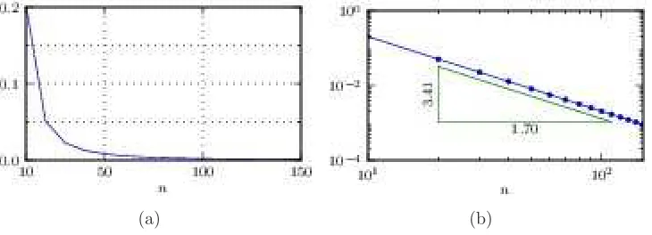
compute kE(vn|c, Yn = Yn′)−v′nkL2(T2) as a function of n and depict it in Figure 2(a). This shows convergence to 0 as predicted. To obtain a rate of convergence, we compute the gradient of a log-log plot of Figure 2(b). We observe the rate of convergence is close to O(n−2). Note that this is higher than the theoretical bound of O(n−φ), with
φ = 1/2∧β, given in Equation (30b); this suggests that our convergence theorems do not have sharp rates.
Finally, we examine the random c′(t, ω′) cases. Figure 1(f) shows the empirical
mean when c′(t;ω′) is chosen such that
Z t
0
(c−c′(s;ω′)) ds=W(t)
where W(t) is a standard Brownian motion. Theorem 4.3 tells us that the computed empirical distribution should have mean close to hui, and this is again the case.
5.3. Sampling the wave velocity and initial condition
The objective of this subsection is to show that the problems caused by model error in the form of a constant shift to the wave velocity can be overcome by sampling cand v0.
We generate data from (12), (13) with c′ = c given by (33) and initial condition (34).
We assume that neither the wave velocity nor the initial condition are known to us, and we attempt to recover them from given data.
The desired conditional distribution is multimodal with respect to c – recall that it is non-Gaussian – and care is required to seed the chain close to the desired value in order to avoid metastability. Although the algorithm does not have access to the true signalv′
n, we do have noisy observations of it: yn′. Thus it is natural to choose as initial
c=c∗ for the Markov chain the value which minimizes
n−1
X
j=1
log
(v′
j+1, φk)
(v′
j, φk)
−2πik·c∆t
2
(a) u(x1, x2) (b)δc= (0,0)
(c) δc= (1/2,1/2) (d)δc= (1/e,1/π)
(e) R∞
0 (c−c
′
(s))ds= (1/2,1/2) (f) Rt 0(c−c
′
(s;ω′
))ds=W(t)
Figure 1. Figure 1(a) is the true initial condition. Figures 1(b) – 1(f) show the desired empirical mean of the smoothing P(v0|Yn =Yn′) for δc= (0,0), δc= (1/2,1/2), δc∈
R\Q×R\Q,R∞
(a) (b) Figure 2. Plot 2(a) shows kE(vn|c, Yn = Y
′
n)−v
′
nk2L2(T2) as a function of n, when
R∞
0 δc(s)ds= (1/2,1/2). Its log-log plot, along with a least squares fit, is depicted in
Plot 2(b), demonstrating quadratic convergence.
Because of the observational noise this estimate is more accurate for small values of k and we choose k= (1,0) to estimate c1 and k = (0,1) to estimate c2.
Figure 3 shows the marginal distribution for ccomputed with four different values of the data sizen, in all cases with the Markov chain seeded as in (35). The results show that the marginal wave velocity distribution P(c|Yn) converges to a Dirac on the true
value as the amount of data is increased. Although not shown here, the initial condition is also converging to a Dirac on the true value (33) in this limit.
We round-off this subsection by mentioning related published literature. First we mention that, in a setting similar to ours, a scheme to approximate the true wave velocity is proposed which uses parameter estimation within 3D Var for the linear advection equation with constant velocity [9], and its hybrid with the EnKF for the non-constant velocity case [10]. These methodologies deal with the problem entirely in finite dimensions but are not limited to the linear dynamics. Secondly we note that, although a constant wave velocity parameter in the linear advection equation is a useful physical idealization in some cases, it is a very rigid assumption, making the data assimilation problem with respect to this parameter quite hard; this is manifest in the large number of samples required to estimate this constant parameter. A notable, and desirable, direction in which to extend this work numerically is to consider the time-dependent wave velocity as presented in Theorems 4.1–4.3. For efficient filtering techniques to estimate time-dependent parameters, the reader is directed to [39, 40, 41, 42].
6. Conclusions
(a)n= 10 (b)n= 50
[image:23.612.112.483.78.496.2](c) n= 100 (d) n= 1000
Figure 3. The marginal distribution of P(c, v0|Yn) with respect to c are depicted
on the square 1.4×10−4 by ×10−4. The red cross marks the true wave velocity c= (−0.5,−1.0).
of the difference in wave velocities. When the difference in wave velocities is constant neither filtering nor smoothing recovers the truth in the large data limit. And when the difference in wave velocities is a fluctuating random field, however small, neither filtering nor smoothing recovers the truth in the large data limit.
There are a number of other ways in which the analysis in this paper could be generalized, in order to obtain a deeper understanding of filtering methods for high dimensional systems. These include: (i) the study of dissipative model dynamics; (ii) the study of nonlinear wave propagation problems; (iii) the study of Lagrangian rather than Eulerian data. Many other generalizations are also possible. For nonlinear systems, the key computational challenge is to find filters which can be justified, either numerically or analytically, and which are computationally feasible to implement. There is already significant activity in this direction, and studying the effect of model/data mismatch will form an important part of the evaluation of these methods.
Acknowledgments
The authors would like to thank the following institutions for financial support: NERC, EPSRC, ERC and ONR. The authors also thank The Mathematics Institute and Centre for Scientific Computing at Warwick University for supplying valuable computation time.
Appendix A. Basic Theorems on Gaussian Measures
Suppose the probability measureµis defined on the Hilbert spaceH. A functionm∈ H is called the mean of µif, for all ℓ in the dual space of linear functionals on H,
ℓ(m) = Z
H
ℓ(x)µ(dx),
and a linear operatorC is called the covariance operator if for allk, ℓ in the dual space of H,
k(Cℓ) = Z
H
k(x−m)ℓ(x−m)µ(dx).
In particular, a measureµis called Gaussian ifµ◦ℓ−1 =N(mℓ, σℓ2) for somemℓ, σℓ ∈R.
Since the mean and covariance operator completely determine a Gaussian measure, we denote a Gaussian measure with mean m and covariance operator C by N(m,C).
The following lemmas, all of which can be found in [29], summarize the properties of Gaussian measures which we require for this paper.
Lemma A.1. If N(0,C) is a Gaussian measure on a Hilbert spaceH, then C is a self-adjoint, positive semi-definite nuclear operator on H. Conversely, if m ∈ H and C is a self-adjoint, positive semi-definite, nuclear operator on H, then there is a Gaussian measure µ=N(m,C) on H.
Lemma A.2. Let H = H1 ⊕ H2 be a separable Hilbert space with projections Πi :
H → Hi, i = 1,2. For an H-valued Gaussian random variable (x1, x2) with mean
m = (m1, m2) and positive-definite covariance operator C, denote Cij = ΠiCΠ∗j. Then
the conditional distribution of x1 given x2 is Gaussian with mean
and covariance operator
C1|2 =C11−C12C22−1C21.
Lemma A.3. (Feldman-Hajek) Two Gaussian measures µi =N(mi,Ci), i= 1,2, on a
Hilbert space H are either singular or equivalent. They are equivalent if and only if the following three conditions hold:
(i) ImC12
1
=ImC12
2
:=E; (ii) m1−m2 ∈E;
(iii) the operator T :=C−12
1 C
1 2
2 C
−12
1 C
1 2
2
∗
−I is Hilbert-Schmidt in E.¯
Lemma A.4. For any two positive-definite, self-adjoint operators Ci, i = 1,2, on a
Hilbert space H, the condition ImC12
1
⊆ ImC12
2
holds if and only if there exists a constant K >0 such that
(h,C1h)≤K(h,C2h), ∀h∈ H
where (·,·) denotes the inner product on H.
Lemma A.5. For Gaussian X on a Hilbert space H with norm k·k and for any integer n, there is constant Cn ≥0 such thatE(kXk2n)≤Cn E kXk2
n .
Appendix B. Proof of Limit Theorems
In this Appendix, we will prove the Limit Theorems 3.2, 3.7, 4.1, whereL=L′,L 6=L′,
L(t)6=L′(t), and Theorem 4.3 where L(t)6=L′(t;ω′), respectively. In all cases, we use
the notations e−tL and e−tL′
to denote the forward solution operators through t time units (from time zero in the non-autonomous case). We denote by M the putative limit for m′
n. The identity
nI+ ΓC−1 0
(m′n−M) = ΓC−1
0 (m0−M) +
n−1
X
l=0
etl+1Lη′ l+1
+
n−1
X
l=0
etl+1(L−L′)u−M
, (B.1)
obtained from Equation (14), will be used to showm′
n →M . In Equation (B.1), we will
choose M so that the contribution of the last term is asymptotically negligible. Define the Fourier representations
en≡m′n−M =
X
k∈K
ˆ
en(k)φk,
ξl ≡etl+1(L−L ′
)u−M =X
k∈K
ˆ ξl(k)φk.
Then M will be any one of u,F(p,q)u,hui and uα.Hence there is C1 independent ofk, l
trivial except in the case of random L′). Using Equation (17), these Fourier coefficients
satisfy the relation
n+ γk λk
ˆ
en(k) =
γk
λk
ˆ
e0(k) +
p γ′
k n−1
X
l=0
(g′k)l+1+
n−1
X
l=0
ˆ
ξl(k), k∈K.
In order to prove m′
n → M in L2(Ω′;Hs(T2)), we use the monotone convergence
theorem to obtain the following inequalities,
nδkenk2L2(Ω′;Hs(T2)) =nδEkenk2Hs(T2)
= X
k∈K+
|k|2snδE|ˆe
n(k)|2+nδE|ˆen(0)|2
= X
k∈K+
|k|2s nδ
(n+γk/λk)2
γk
λk
2
|ˆe0(k)|2+γ′
kn + 2Re ( γk λk ¯ˆ
e0(k)E
n−1
X
l=0
ˆ ξl(k)
!) +E
n−1
X
l=0
ˆ ξl(k)
2 + n δ
(n+γ0/λ0)2
"
γ0
λ0
2
|ˆe0(0)|2+γ0′n
#
≤ X
k∈K+
|k|2snδ−2 γk
λk
2
|ˆe0(k)|2
+γk′n+ 2C1
γk
λk|
ˆ
e0(k)||(u, φk)|n+E
n−1
X
l=0
ˆ ξl(k)
2
+nδ−2 "
γ0
λ0
2
|eˆ0(0)|2+γ0′n
#
≤ X
k∈K+
|k|2snδ−2 γk
λk
2
|ˆe0(k)|2+γk′n
+C1
γk
λk
2
|ˆe0(k)|2+|(u, φk)|2
!
n+E
n−1
X
l=0
ˆ ξl(k)
2
+nδ−2 "
γ0
λ0
2
|eˆ0(0)|2+γ0′n
#
≤Ckm0−MkHs+κ(T2)
nδ−2+ X
k∈K
|k|2sγ′k !
nδ−1
+C1kukHs(T2)
nδ−1+
X
k∈K+
|k|2snδ−2E
n−1
X
l=0
ˆ ξl(k)
2
≤Ckm0kHs+κ(T2)+kukHs+κ(T2)
+ X
k∈K
|k|2sγ′
k+C1kukHs(T2) !
nδ−1
+
X
k∈K
|k|2snδ−2E
n−1
X
l=0
ˆ ξl(k)
2
, (B.2)
and here the first two terms in the last equation can be controlled by Assumptions 3.1. In order to find δ∈[0,1] such that this equation isO(1) or o(1),
X
k∈K
|k|2snδ−2E
n−1
X
l=0
ˆ ξl(k)
2 (B.3)
is the key term. This term arises from the model error, i.e., the discrepancy between the operator L used in the statistical model and the operator L′ which generates the
data. We analyze it, in various cases, in the subsections which follow. In order to prove m′
n →M in Hs(T2), Ω′ −a.s., suppose we have
1 n
n−1
X
l=0
ˆ
ξl(k)→0 Ω′−a.s., (B.4)
for each k ∈ K. We then use the strong law of large numbers to obtain the following inequalities, which holds Ω′−a.s.,
kenk2Hs(T2) = X
k∈K+
|k|2s|ˆen(k)|2+|eˆn(0)|2
= X
k∈K+
|k|2s
(γk/λk) ˆe0(k) +
p γ′
k
Pn−1
l=0(g′k)l+1+
Pn−1
l=0 ξˆl(k)
n+γk/λk
2 +
(γ0/λ0) ˆe0(0) +
p γ′
0
Pn−1
l=0(g′0)l+1
n+γ0/λ0
2
≤ CX
k∈K
(1 +|k|2s)
(γk/λk) ˆe0(k)
n 2 + p γ′ k
Pn−1
l=0(gk′)l+1
n 2 +
Pn−1
l=0 ξˆl(k)
n 2
≤ CX
k∈K
(1 +|k|2s) |k|2κ|ˆe
0(k)|2+γk′ +|(u, φk)|2
≤C km0kHs+κ(T2)+kukHs+κ(T2)+ X
k∈K
|k|2sγ′
k+kukHs(T2) !
. (B.5)