Faculty of Engineering Technology
Multilevel Panel Method
Validation Using the New
MEXICO Wind Tunnel
Measurements
Erik Prieto S.
M.Sc. Thesis
November 2017
Supervisors:
prof.dr.ir. C.H. Venner. dr.ir. A. van Garrel
To my father, my mother and my brother with all my love.
Acknowledgements
I would like to thank first to my supervisors Arne van Garrel and Kees Venner, for the enlightenment through this work, their teaching and ideas fed my curiosity for the fluid dynamic field. Their sharp comments and optimistic advice were the fuel and the fire that helped me to get which I desire.
Special thanks to Arne van Garrel who devoted their time and patience unconditionally and punc-tually every Thursday morning through all the thesis, with talks about the future of the world without sustainability and renewable energies, who also teach me the multilevel panel method spiny details, for sharing his experience in the aerodynamic field, and finally for offering me his honest friendship.
My total gratefulness to Kees Venner for accepting me as part of his research group, for helping me in the darkest moments of my master, who provided me with all the necessary tools to develop the knowledge by my self, who take the time to care about his students and finally for offered me the opportunity of doing my internship at GE, where I had an incredible and rich experience.
My gratitude to the committee for this examination for taking the time to read my work and give their comments, my two supervisors, prof.dr.ir. C.H. Venner, and dr.ir. A. van Garrel. the prof. ir. Theo van der Meer and from ECN the Dr. ir, Koen Boorsma.
My thanks to Saskia Honhoff, who was my supervisor at GE and who make my stay during the short period of time a wonderful experience, not just as a critical supervisor but as a friend and a colleague.
I want to express my gratuity to the Science and Technology Council of Mexico (Consejo Nacional de Ciencia y Tecnolog´ıa, CONACYT) that has granted me with the scholarship throughout my Master of Science Program, and all the people there that helped me with all my academic and financial issues.
None of this would be possible without my dear friend Leonel Reyes who encourage me to pursue my master degree, his advice, reprimanding, his share of experiences and faith on my work have helped me in the most difficult moments.
During my master, I have the privilege to get to know many wonderful persons. I am indebted to my friend Lorena for several discussions that helped me to be not just a robot but also a human being. Also, I want to thank all my SET friends for giving their opinions and comments on other
It must also be acknowledged all the people in M´exico who has maintained the time to care about my studies. My debt to the Dr Miguel de Icaza Herrera, who is not just the best physic professor I ever had, but also an endearing friend. Also to my dear Mar who has always believed in me. I thank all my friends around the world, who has made this experience a little bit less scary.
Last but not the least, I would like to thank my family: my parents Angel Prieto and Micaela Serratos, and my brother Ovidio for giving not just economical support but also supporting me spiritually throughout my life.
Summary
The human activities nowadays have a huge impact in the world. The best known consequence is “climate change” that is heavily related to our excessive consumption of natural resources. This provokes numerous problems like the production of green house gases that trap heat in the atmosphere and change the natural climate conditions on earth. As the dominant species on the planet, there are a lot of solutions that we can implement to fight climate change. Solutions like population reduction through sexual education, smart food production practices, better energy policies, recycling, circular economies, and renewable energy production are some examples.
Increasing the use of renewable energies such as solar, biomass and wind power is a relevant and important strategy nowadays for combating climate change due the rising energy consumption in the world. There is no single solution to climate change but rather a combination of several solutions is necessary. Particularly in the energy field interesting solutions can be used. Among all the energy solutions, wind energy is catalogued as the second most influential solution to reduce CO2 emissions just after “Refrigerant Management”. Wind energy keeps growing and new developments are carried out constantly in all areas. Several developments are related to the correct prediction of aerodynamic phenomena that are present in the extraction of energy from the wind.
Developments in the aerodynamic theory help to predict the forces acting on the wind turbine and improve the power production of the turbines. The blade element momentum (BEM) theory is one of the earliest aerodynamic theories for wind turbines and is still in use nowadays. The more advanced methods are based on Reynolds-Averaged Navier-Stokes (RANS) equations and make use of turbulent models or even resort to Large Eddy Simulation (LES) [1].
Some of these methods constitute what is known as Computation Fluid Dynamics (CFD), a field that has a wide range of methods to solve fluid flow problems. Generally these methods involve complicated mathematical and numerical approaches and while being accurate their application is computationally expensive and too slow for use in day to day design practice.
In this thesis the validation of a so-called ‘Multilevel Panel Method’ is performed. The panel method is an attractive flow analysis technique that, in contrast to other CFD methods, is computationally efficient and still has fundamental physics involved to work out the solutions. The validation is performed using the results from a European wind tunnel experiment called “New MEXICO”. We demonstrate the fidelity of the advanced multilevel panel method under unsteady conditions. We consider cases with rotor yaw at angles −30◦, 15◦, 30◦ and 45◦, and two types of step changes:
This thesis concludes by giving some recommendations for further validations and the use of the state-of-the-art multilevel panel method.
Contents
Acknowledgements V
Summary VII
Contents XI
Nomenclature XIX
1 Introduction 1
1.1 Context . . . 1
1.1.1 Climate Change and Global Warming . . . 1
1.1.2 Mitigating the Effects of Human Behaviour . . . 5
1.1.3 Wind Energy and Wind Turbines . . . 6
1.1.4 Aerodynamic Theories on Wind Energy . . . 8
1.2 Problem Statement . . . 10
1.3 Objectives . . . 10
1.4 Approach . . . 10
1.5 Thesis outline . . . 11
2 Multilevel Panel Method 13 2.1 Introduction . . . 13
2.2 Governing Equations . . . 14
2.2.1 Boundary Integral Equation . . . 15
2.2.2 Boundary Conditions . . . 16
2.2.2.1 Body Surface . . . 16
2.2.3 Wake Surface . . . 18
2.2.4 Pressure Coefficient Definition . . . 19
2.2.5 Panel Method . . . 20
2.3 Multi Level Multi Integration Cluster Scheme . . . 22
3 New MEXICO Wind Tunnel Experiment 25 3.1 Introduction . . . 25
3.2 Definition and Conventions . . . 26
3.3 Wind Turbine . . . 28
3.4 Wind Tunnel . . . 30
3.5 Measurments and Instrumentation . . . 31
3.5.1 Data Acquisition . . . 31
3.5.2 Uncertainty of Pressure Sensors . . . 32
3.5.3 Measurement Data Points . . . 33
3.6 Data Selection for Validation . . . 33
4 Panel Method Validation 37 4.1 Introduction . . . 37
4.1.1 Simulation Panels . . . 39
4.1.2 Effect of Reference Velocity on Pressure Coefficients . . . 40
4.2 Yawed Rotor Cases . . . 44
4.2.1 Yaw Angle15◦ . . . 44
4.2.2 Yaw Angle30◦ . . . 52
4.2.3 Yaw Angle−30◦. . . 59
4.2.4 Yaw Angle45◦ . . . 66
4.3 Dynamic Inflow Cases . . . 73
4.3.1 Step in Blade Pitch Angle . . . 73
4.3.1.1 Sensors With Time Delay . . . 79
4.3.2 Step in Rotor Angular Velocity . . . 80
4.3.2.1 Rotor Speed Conversion . . . 81
5 Conclusions and Recommendations 89 5.1 Conclusions . . . 89
5.2 Recommendations . . . 90
References 97 Appendix 99 A Matlab Routines . . . 100
A.1 File Processing file . . . 100
A.2 RPD name extraction . . . 104
A.3 Arrange . . . 106
A.4 Azimuth Average . . . 107
A.5 Time series values with columns arrangement . . . 126
A.6 Time series values with rows arrangement . . . 145
B Complete correlation of configurations and files for the New MEXICO experiment . 164 C Kulite®Sensors Data Information . . . 166
D Example of file generated with Matlab routine . . . 167
List of Figures
1.1 Hockey stick graph . . . 3
1.2 Hurricane Irma . . . 4
1.3 Three hurricanes . . . 5
1.4 Wind turbines . . . 6
1.5 World wind capacity . . . 8
1.6 Big turbines . . . 9
2.1 Flow domain . . . 15
2.2 Panel and node ordering . . . 21
2.3 Panels over blade. . . 21
2.4 Multi level concept . . . 22
3.1 Azimuth angle, yaw, and coordinate system definitions [63]. . . 27
3.2 Pitch angle definition. . . 27
3.3 Airfoil sections . . . 29
3.4 Blade composition shape from [63]. . . 29
3.5 Schematic view of LLF tunnel . . . 30
4.1 Azimuth averaging locations . . . 38
4.2 Rotor geometry and wake . . . 40
4.4 Effects of Non-dimensionalization in Cp . . . 43
4.5 15◦ Yaw, azimuth angle 0◦ . . . 46
4.6 15◦ Yaw, azimuth angle 60◦ . . . 47
4.7 15◦ Yaw, azimuth angle 120◦ . . . 48
4.8 15◦ Yaw, azimuth angle 180◦ . . . 49
4.9 15◦ Yaw, azimuth angle 240◦ . . . 50
4.10 15◦ Yaw, azimuth angle 300◦ . . . 51
4.11 30◦ Yaw, azimuth angle 0◦ . . . 53
4.12 30◦ Yaw, azimuth angle 60◦ . . . 54
4.13 30◦ Yaw, azimuth angle 120◦ . . . 55
4.14 30◦ Yaw, azimuth angle 180◦ . . . 56
4.15 30◦ Yaw, azimuth angle 240◦ . . . 57
4.16 30◦ Yaw, azimuth angle 300◦ . . . 58
4.17 −30◦ Yaw, azimuth angle 0◦ . . . 60
4.18 −30◦ Yaw, azimuth angle 60◦ . . . 61
4.19 −30◦ Yaw, azimuth angle 120◦ . . . 62
4.20 −30◦ Yaw, azimuth angle 180◦ . . . 63
4.21 −30◦ Yaw, azimuth angle 240◦ . . . 64
4.22 −30◦ Yaw, azimuth angle 300◦ . . . 65
4.23 45◦ Yaw, azimuth angle 0◦ . . . 67
4.24 45◦ Yaw, azimuth angle 60◦ . . . 68
4.25 45◦ Yaw, azimuth angle 120◦ . . . 69
4.26 45◦ Yaw, azimuth angle 180◦ . . . 70
4.27 45◦ Yaw, azimuth angle 240◦ . . . 71
4.28 45◦ Yaw, azimuth angle 300◦ . . . 72
4.29 Pitch step plot . . . 73
4.30 Pitcht1 = 4.65s . . . 75
4.31 Pitcht2 = 5.20s . . . 76
4.32 Pitcht3 = 10.85s . . . 77
4.33 Pitcht4 = 11.25s . . . 78
4.34 RPM step plot . . . 80
4.35 RPM integration . . . 82
4.36 Velocity triangle changes for 424 rpm and 324 rpm. . . 83
4.37 Pitcht1 = 3.63s . . . 84
4.38 Pitcht2 = 5.68s . . . 85
4.39 Pitcht3 = 9.67s . . . 86
4.40 Pitcht4 = 11.88s . . . 87
List of Tables
1.1 Increase factor of human activities during the 20th century. . . 2
3.1 General turbine information, modified from [63]. . . 28
3.2 Position of pressure sensors at blade and radial location . . . 31
3.3 Estimated pressure coefficient due to uncertainty in the pressure sensors . . . 32
3.4 Correlation of data for cases used for the validation . . . 34
B1 Model configuration legends for the New MEXICO . . . 164
B2 Correlation of data for cases and files of the New MEXICO experiment . . . 165
C1 Specifiactions of Kulite® XCQ-95-062-5A. . . 166
D1 Example of file generated with Matlab routines. . . 167
Nomenclature
Dimensions
[kg] kilogram mass [m] meter length [s] second time
[rad] radian angle [m·m−1]
[−] dimensionless
Acronyms
AoA Angle of Attck BC Boundary Condition BEM Blade Element Momentum CFD Computational Fluid Dynamics
DNW German-Dutch Wind Tunnel Organisation ECN Energy research Centre of the Netherlands LES Large Eddy Simulation
LLF Large Scale Low-Speed Facility
MG Multigrid
MEXICO Model Experiments in Controlled Conditions MLMIC Multi Level Multi Integration Cluster
RaNS Reynolds-averaged Navier-Stokes RPM Revolutions Per Minute
VII Viscous-Inviscid Interaction
Cp [−] pressure coefficient
c [m] chord length
i, j [−] index numbers
L [m] length
Ma [−] Mach number
N [−] problem size
n [−] number of elements
P [W] power
p [N·m−2] pressure
Re [−] Reynolds number
t [s] time
U [m·s−1] velocity v [m·s−1] velocity
∂S [m] surface boundary ∂V [m2] volume boundary x, y, z [m] Cartesian coordinates
Greek symbols
α [rad] angle of attack
δ,∆ [m] length scales
∆ [−] difference
Φ [m2·s−1] velocity potential
ϕ [m2·s−1] velocity perturbation potential Γ [m2·s−1] vortex strength
λ [−] local speed ratio, scaling factor, wing aspect ratio µ [kg ·m−1·s−1] dynamic viscosity coefficient
µ [m2·s−1] dipole strength ν [m2·s−1] kinematic viscosity
Ω [· · ·] space
Ψ [· · ·] scalar field
Ψ [◦] azimuth angle location ψ [· · ·] scalar field
ρ [kg·m3] mass density σ [m·s−1] source strength
θ [rad] rotation angle
χ [◦] amount of degrees travelled by a blade.
Vectors, matrices, and tensors
~
Ω [rad ·s−1] angular velocity vector ~
ωv [s−1] volume vorticity distribution ~u [m·s−1] velocity vector
~x [m] point location ~y [m] point location
Chapter 1
Introduction
You who read me, are you sure of understanding my language?
Jorge Luis Borges, The Library of Babel
1.1
Context
1.1.1 Climate Change and Global Warming
Human activities have grown in the last three centuries at impressive rates, world population has grown by a factor of four [2], the industrial output grew by a factor of 40 [2]. This was accompanied by an increase in energy use by a factor of 16 just during the 20th century alone. As consequence nearly 66% of atmospheric and ocean rise temperature can be confidently attributed to human activities [3]. The radical example of the decreasing of the blue whale population by 99.75% is one of many examples of how human activities exert an increasing impact on the environment on all scales [2]. Some other impacts of human activities during the 20th century can be seen on the Table 1.1.
The most known consequence of the human activities is “climate change”. The causes are heavily related to the human activities [4–6], from unprecedented warming [7–10] to heavy snowfalls like the North American blizzard that occurred on the 5-6 of February 2010 [11]. Although some major climatic events happened before [6], it seems that nowadays the main drivers are us humans ourselves. The addiction to the consumption of natural resources like the burning of coal and oil produces so called “green house gases” (GHG) [12], gases that trap heat in the atmosphere, thus changing the natural climate conditions on earth.
Carbon dioxideCO2 and methaneCH4 are two harmful greenhouse gases [13–15]. The greenhouse gas CO2 expelled into the atmosphere through burning fossil fuels like coal, natural gas and oil.
Table 1.1: A partial record of the growths and impacts of human activities during the 20th century, from [2]
Item Increase Factor,
1890s-1990s
World population 4
Total world urban population 13
World economy 14
Industrial output 40
Energy use 16
Coal production 7
Carbon dioxide emissions 17 Sulphur dioxide emissions 13
Lead emissions ≈8
Water use 9
Marine fish catch 35
Cattle population 4
Pig population 9
Irrigated area 5
Cropland 2
Forest area 20% decrease
Blue whale population (Southern Ocean) 99.75% decrease Fin whale population 97% decrease Bird and mammal species 1% decrease
Burning wood products, solid waste and trees, and even the result of certain type of chemical reactions, for example manufacturing cement, contribute to the amount of releasedCO2. Over the last 200 years: the amount of CO2 in the atmosphere has increased more than 30% and CH4 by even more than 100%. As a result, an increase of 0.5 degrees Celsius in average global temperature in the past century has been observed [2]. Methane is emitted during the production and transport of oil, coal, and natural gas. Another source of the methane emissions is the result of livestock and other agricultural practices. Carbon dioxide accounts for the 82% of all greenhouse gas emissions and methane is the second most prevalent greenhouse emitted by human activities in the U.S.A. [13, 16], despite that methane only accounts for 9% of total greenhouse gas emissions methane is a more potent greenhouse gas thanCO2 [16, 17].
To asses a comparison between the impact of different gases, the Global Warming Potential (GWP) is used. The GWP specifically measures how much energy the emission of 1 ton of gas will absorb over a given period of time, using CO2 as comparison over that time period [18]. The larger GWP, the more the earth warms compared to CO2. One hundred years is the usual period of time chosen for this comparison. CO2 has a GWP of 1 by definition while methane has a GWP of 28–36 over 100 years. Methane last about one decade on average but absorbs much more energy than CO2 and similar, to carbon dioxide, methane has natural processes that remove it from the atmosphere. However, these natural processes can not remove these greenhouse gases at the same rate the amount of gases are produced nowadays.
1.1. CONTEXT 3
It is argued that near-term climate changes need to be viewed on a long-term perspective to emphasise the severity of this problem, and consciousness should be raised to the fact that climate change will extend longer than the entire history of the human civilisation [19].
The increase in the average temperature due to global warming1[9, 10] could lead to a global risk of deadly heat waves [20], with associated mortality that can be attributed to this climate change [21]. The effect of global warming is shown dramatically in a figure with the famous hockey stick (see Figure 1.1 ), a graph describing the reconstruction of the temperature over the past 1000 to 2000 years using tree-rings, ice cores, coral and other records that act as proxies for temperature. This reconstruction found that global temperature gradually cooled over the past millennia with a sharp upturn in the 20th century. The main result from the paper [22] is that global temperatures over the last few decades are the warmest in the last 100 years. The effects of this warming are not just restricted to the human species but also to plants and non-human animals where local extinction is already happening [23]. It is really important to make people aware of the dangers that we are facing and realise that the human beings can not survive without a biodiverse environment.
Figure 1.1: Hockey stick graph from [22].
Effects in the ecosystem are visible now, like the calving event of the Larsen-C ice shelf, the largest remaining ice shelf on the Antarctic peninsula [24], or the weakening of the Atlantic Meridional Overturning Circulation, a large-scale circulation pattern in the Atlantic that plays a important role as a heat and freshwater transport, having a directly influence on climate change [25].
Currently, hurricanes grow in severity reaching 300 km/h wind speed, increasing the frequency of occurrence or the size with super hurricanes like Irma shown in the Figure 1.2. Formation of such hurricanes is heavily related to the increased water temperatures in the Atlantic and Pacific Ocean. The frequency of these type of events is also increasing: at the same time Irma hit the south of Florida, another hurricane was hitting the cost of Mexico, and a third one was approaching with probably the same outcome (see Figure 1.3).
1
Figure 1.2: Geocolor Image of Hurricane Irma passing the eastern end of Cuba at about 8:00 a.m. EDT on Sept. 8, 2017, Courtesy of NASA.
The human extraction of natural resources for consumption purposes or for commodities has many key points, one of those is the production of meat at industrial scale farms since this represents the number one-driver of tropical deforestation in south America and worldwide with a nearly 60% of embodied deforestation [26, 27]. The second large driver of deforestation2 is soy production, accounting for 19% of global deforestation reported within 1990 and 2008 [28]. However, the majority (around 70 to 75% of the world’s soy) goes to feed cows, chickens, pigs, and farmed fish [27, 28], accounting for the meat production. Another example is that half of all accessible fresh water is used by mankind, and all these activities (the increasing of fossil fuel burning, agricultural activities, deforestation, and intensive cattle raising) have increased the number of several greenhouse gases (GHG) in the atmosphere. According to [29] the livestock sector generates more greenhouse gas emissions as measured in CO2 equivalent than all cars, planes, trains, ship and trucks together [30].
This generates positive feedback loops, which can be seen as a vicious circle that accelerates the warming trend (a negative feedback loop will decelerate the warming trend). These positive feed-back loops are well know, one example is the melting of ice due the warming temperature. The ice is light-coloured and reflective, acting as a mirror and reflecting a large portion of the sunlight that reaches the earth, thus reducing the amount of warming that this causes. The melting of the ice due the warming reduce white ice surface and increase the “darker-coloured” land and sea water below it. The result is the increase of energy absorbed which lead to more warming that turns out to more ice melted etcetera. These positive feedback loops affect the artic tundra and heating of the arctic coastal waters resulting in additional release of methane, a very potent greenhouse gas that contributes to the problem as well. It is of vital importance to have negative feedback loops related to the human activities.
2
1.1. CONTEXT 5
Figure 1.3: Three Hurricanes heading east cost of America cuba and Mexico. Courtesy of NASA.
1.1.2 Mitigating the Effects of Human Behaviour
Many efforts have been made to mitigate the impact of human behaviour for example the creation of the Intergovernmental Panel on Climate Change (IPCC) in 1988 as a scientific and intergovern-mental body dedicated to providing the world with an objective scientific point of view of climate change and its political and economic impacts [31]. In particular for the fifth assessment report (AR5), the probability of global mean temperatures exceeding the 1.5◦C and 2◦ C above 1850-1900 levels was estimated, leading to catastrophic effects for the future life on the earth. This report has been used to generate several scenarios to predict future outcomes depending on the measures taken today [32]. Another important effort is the Kyoto Protocol which took place the 11 of De-cember of 1997, where the industrialised countries agreed to apply a set of mandatory targets on GHG emissions. These countries agreed to reduce the mean average of pollutant emissions between 2008 and 2012 by 5.2% taking as a reference the levels of 1990. The protocol entered into force on 16 February 2005 after the ratification by Russia the 18 of November of 2004. However, the USA signed the protocol but did not ratify, even when the USA is the second emitter of CO2 in the world [33].
The most recent example of the efforts is the so called COP21 which was held in Paris in December 2015, the COP21 result in the agreement of 195 countries to keep global temperatures below 2.0◦C above pre-industrial3 times and “endeavour to limit” them even more, to 1.5◦ C[34]. Although the agreement was initially seen like a major change towards the improvement of the climate change, in 2017 the USA president decided to withdraw from the agreement, this represent a draw back in the mutual objective of reduce the effects of the climate changes. Thus it is necessary to work
3
harder and better to overcome all the obstacles and give more precise data and information about the effects of the climate change. Despite the bad news on powerful economies and actors against climate change mitigation there still a wider spectrum of attempts to reduce the emission related to human activities in several possible fields. These fields include; energy, food and water, women and girls, buildings and cities, land use, transport and materials, etc. There are many different ways to oppose the effects of global warming and climate change like the capture and storage of carbon, the use of bioenergy, the combination of these two is known as BECCS (Bioenergy Combined with Carbon Capture and Storage) [35]. Other measurements are the recovery and protection of land by means of protective policies [36], the reduction of flight time per year per person [37], improvement on the methods of construction using alternative cement [36], and the reduction of the use of fossil-fuels as main source of energy.
1.1.3 Wind Energy and Wind Turbines
Among all the solutions to reduce the release of greenhouse gases in the atmosphere, one of the most important aspects is the generation of clean energy, when renewable energy sources like solar, tidal, geothermal and others are implemented. The use of these type of technologies seeks to reduce the use of fossil fuels, even though the use of the fossil-fuels seems to be an addictive habit that is going to be with humans for a long period. The impact of the implementation of new renewable energy technologies will help to reduce pollution and the emission of greenhouse gases.
From all the types of renewable energy and measures to address global warming, wind energy (onshore) is catalogued as the second most influential solution to reduce CO2 emissions on a plausible scenario for 2050 just after “Refrigerant Management” [? ]. The impressive number of wind turbines nowadays is astonishing, by the end of 2016, 4% of global electricity demand was covered by 341,320 wind turbines [38].
1.1. CONTEXT 7
The use of the wind as a source of energy has being practised for centuries4, for example the vertical axis windmills found at the Persian-Afghan border around 200 BC, the horizontal-axis windmills of the Netherlands and the Mediterranean, and of course all the sailing boats powered by wind energy mentioned since Odysseus, the greeks, vikings and many other cultures who use wind to move across the seas [39].
Windmills got further improvements that were developed in the USA during the 19th century. However, it was not until the notable work in aerodynamics by Betz in Germany and Lancaster in England that allowed subsequent efforts in Denmark, France, Germany, and the UK (during the period between 1935 and 1970), and showed that large-scale wind turbines could work [39, 40].
With the realisation of this idea, wind turbines were installed and its re-emergence as an important source of energy for the world became one of the most significant developments of the late 20th-century [41] in such way that at the end of 2016 the global cumulative installed wind power capacity was 486,790 MW, with China, USA, Germany, India and Spain among the top five countries with 34.7%, 16.9%, 10.3% 5.9% 4.7% of the share respectively [42]. During 2015 a record of 63,467 MW of wind power was installed around the world, and during 2016, the amount of wind power installed was of 54,642MW around the world [42]. In Figure 1.5 the share of the cumulative capacity of wind energy installed is shown.
For the specific case of the Netherlands, the wind energy installation broke records in 2016, entering the global top 10 in terms of annual market for the first time in decades. Installing 887 MW in 2016, ending with a total of 4.32 GW, accounted for the 8.9% country’s electricity demand [42].
With the proliferation of turbines, the reduction of costs, the high performance of the turbines, the wind industry is growing. With future cost-reductions wind energy will be the least expensive source of electricity within a decade [43, 44]. Wind farms onshore usually have a small footprint, using around 1% of the land they sit on, so other activities can happen simultaneously with power generation, like farming, grazing and recreation. Moreover, the time required to build a wind farm is between 2 months and 1 year (depending on the capacity of the wind farm) [45] giving the advantage of quickly producing energy and return on investment.
Like other renewable energy technologies, energy production by means of wind turbines depends on weather or seasonal conditions and is not completely constant. Thus it is important to invest in 24-7 renewables such as geothermal and in energy storage and transmission infrastructure.
Some scenarios forecast a CO2 reduction of 84.6 gigatons by 2050 just increasing the world elec-tricity use base on wind energy from 4% to 21.6%, with an estimated cost ofe1.03 trillion within 30 years of operation. Under conservative estimates this could result in ae6.2 trillion net savings not including new technological developments and cost reductions which eventually will lead to an increase in capacity to generate more electricity at lower cost using wind power [36, 43].
Wind energy is an option to help reduce the effects of climate change, however, this is not the master solution. In fact, there is not a single solution to stop or reduce climate change, at most, the only viable solution is the combination of several solutions to reduce and fight climate change.
4
Figure 1.5: World cumulative capacity 2016 courtesy of GWEC [42].
1.1.4 Aerodynamic Theories on Wind Energy
Developments in many areas of technology were adapted for application to wind turbines. This helped to the re-emergence of this technology to make it more reliable, more cost effective, and quieter. Areas like power electronics, analytical design and analysis methods, computer science, materials science, testing and monitoring, and aerodynamics benefited from these developments. The topic of aerodynamics was originally a development for aerospace industry but has now been adopted by the wind industry. Developments in the aerodynamic theory help to predict the forces acting on the wind turbine and improve the power production of the turbines. However, the blade element momentum (BEM) theory, one of the earliest aerodynamic theories for wind turbines is still in use nowadays. It is a method based on dividing the flow in annular control volumes and then apply a momentum balance and energy conservation to each control volume. The vortex-lattice and vortex-particle methods assume incompressible, inviscid flow and attempt to describe it with either vorticity sheets or vortex particles. The most advanced methods, are based on Reynolds-Averaged Navier-Stokes (RANS) equations and make use of turbulent models or even resort to Large Eddy Simulation (LES) [1].
1.1. CONTEXT 9
Figure 1.6: Big turbines (Representative size, height, and diameter of wind turbines (Steve Connors, MIT) )
that has a wide range of methods to solve fluid flow problems. However, CFD methods like RANS or LES solvers, although accurate, tend to be expensive (in time and money). If unsteady considerations are taken into account the computational time could extend to months for a fully described wind turbine solution. On top of that, the trend of the continuous growth of the wind turbines (Figure 1.6) make it even more difficult to perform accurate and fast simulations. With this in mind, is necessary to find some other method that can help to make accurate predictions, in which computation time is reduced, but an adequate level of physics in the description is maintained.
The panel method is an attractive flow analysis technique that, in contrast to other CFD methods, is not expensive and still has fundamental physics involved to work out the solutions. This is a tool of choice for wind turbine and propeller simulations, its major advantage. Its the ability to rapidly simulate complex configuration with large wakes in external flow domains. Another advantage of the panel method is that the discretisation is made in the surface elements only, meaning a much faster and simple meshing.
However, the panel method does not model viscosity, compressibility, and distributed volume vor-ticity, although some additional models allow a degree of correction in the compressible case. With boundary layer simulation the effect of viscosity can be artificially accounted for [46].
wing (and by extension on a wind turbine blade) as long as the viscous effects are negligible (away from stall conditions). The panel method requires a wake shed from the wing trailing edge in order to predict lift. As soon as the trailing edge is identified the wakes can be generated automatically. If there is no wake defined, the panel method operates in its pure non-lifting inviscid mode.
The panel method is a valuable tool for the analysis of fully attached subsonic flows with high Reynolds number. More about this method and the complete description can be found in Chapter 2.
1.2
Problem Statement
Despite the accuracy of CFD methods, those are usually expensive methods to solve and predict the turbine behaviour in unsteady problems, so it is necessary to come with a fast solution that still involves a adequate physics for the solution. In particular for unsteady flow cases, an efficient option is the panel method, which solves the problem to engineering accuracy and is not that computationally expensive. This method has shown a good match with experiment for steady cases [48]. In this thesis we analyse and validate the accuracy of the method described in [48] for unsteady flow cases.
1.3
Objectives
This thesis work will focus on the validation of the multilevel panel method code developed in [48]. Specific points will be discussed in this thesis.
1. Validate the multilevel panel method using the database of results from the New MEXICO wind tunnel experiment.
• Validation of the accuracy of the method under the unsteady conditions.
• Discuss the possible flow cases, areas of application and disadvantages of the method for wind turbine aerodynamics simulations.
2. Generate a base work for future projects using the routines and codes for the extraction of the information of the New MEXICO experiment.
1.4
Approach
1.5. THESIS OUTLINE 11
numerical simulations. It is then easy to compare the experimentally and numerically obtained values of the pressure coefficients as function of dimensionless chord wise position.
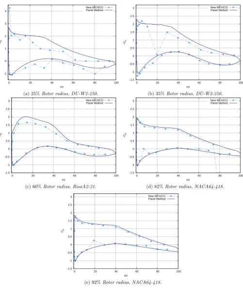
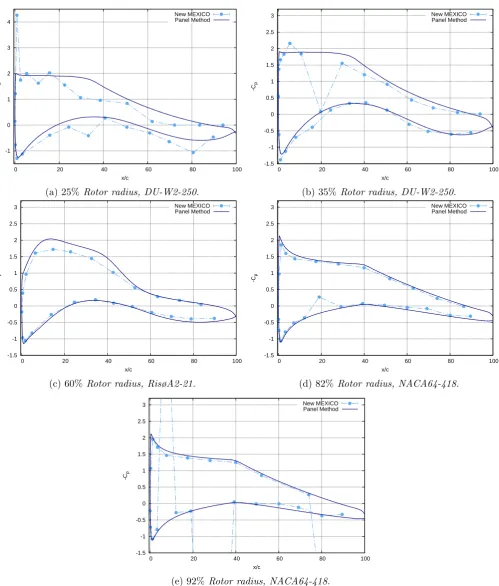
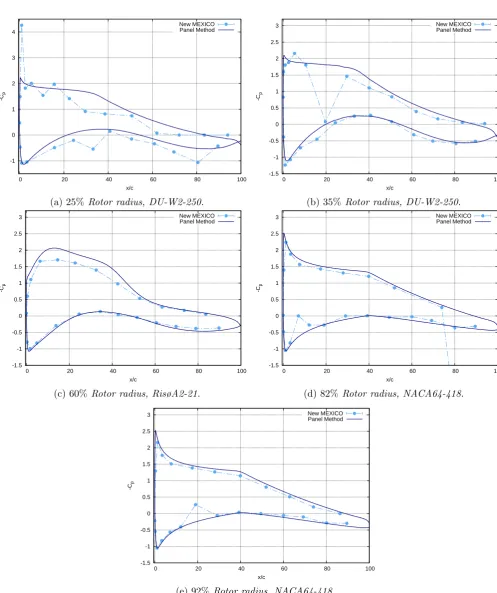
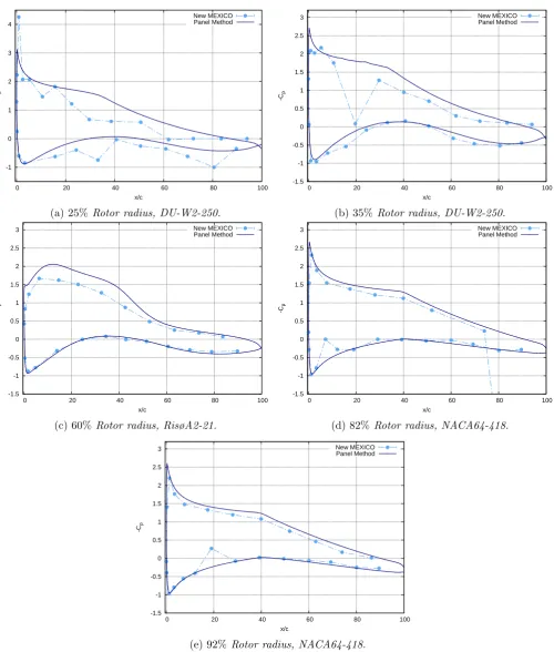
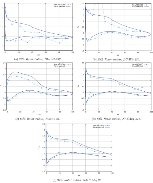
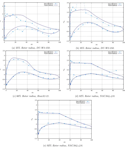
The selected radii for the comparison of pressure distribution followed the sensor locations of the MEXICO and New MEXICO experiments, being at 25%, 35%, 60%, 82% and 92% of the radius. The experimental data consists of several gigabytes of information. From the available pressure data the yaw cases were selected for the validation of the multilevel panel method (among with other cases to verify limitation of such method).
For a fixed set of azimuth angles [0◦,60◦,120◦,180◦,240◦,300◦] the pressure data was collected from the database. For each azimuth position an ensemble average was determined for all 5 airfoils sections. The five chord-wise pressure distributions for each specific azimuth angle will be used for the validation of the multilevel panel method as described in Chapter 4. Some time dependent compilations were made for the cases of the pitch ramp and for the step in rotor speed.
Finally the comparison was made among the simulated values with the extracted value of the experiment.
1.5
Thesis outline
Chapter 2
Multilevel Panel Method
“If the honor and wisdom and joy of such a reading are not to be my own, then let them be for others. Let heaven exist, though my own place be in hell.
Jorge Luis Borges, The Library of Babel
2.1
Introduction
In 1962 Hess and Smith [49] published a paper called “Calculation of Non-lifting Potential Flow About Arbitrary Three-Dimensional Bodies” which as the title indicates, explores a general method for computing the incompressible potential flow about arbitrary, non-lifting, three-dimensional bodies. This is considered a pioneer work in the 3D panel methods field, which in fact could also be considered as a pioneer work in the entire CFD field too.
From the theoretical methods available the panel method is one of the most versatile methods from the user’s point of view. The method is commonly known as “panel method”, but also sometimes known as “boundary integral” or “surface singularity” method, even sometimes is called “boundary element method”. Nowadays the boundary element method is known in the wind energy field under the classic name of “panel method”, since it could be confused with the blade element momentum method, also related to wind turbine aerodynamics, that shares the same acronym (BEM). Therefore the name “panel method” will be used throughout this thesis in order to avoid confusions.
Since the work of Hess and Smith, the panel method has evolved and there exist many types of panel methods. However, the main principle of the method remains unchanged, that is “covering the surface with singularity elements”, which is the main advantage of the panel method since the problem is reduced to an integral equation on the surface of the geometry only. Therefore, no volume discretisation is required [46]. As a result the method can handle easily numerical
simulations of relatively complicated geometries rather easily.
The shortcomings of the panel method are connected with the assumption of inviscid potential flow. Standard panel methods, do not model viscosity, strong non-linear compressibility and volume distributed vorticity. This inability to simulate high-speed transonic flows, allow methods based on the unsteady Navier-Stokes equations1 like RANS or LES to be used in the field of CFD. However, the panel method is still being considered an engineering tool of choice for wind turbine and propeller simulations. The major advantage for these flow problems lies in the ability to rapidly simulate configurations with large and complex wakes in external flow domains [46].
In this thesis we give a concise description of the panel method developed in [48]. For a more thorough discussion the reader is referred to the original work.
2.2
Governing Equations
For the description of the panel method it is necessary to have certain physical considerations. First, the normal operation of the wind turbine will be in which the local flow velocities occurring at the rotor blades are at most 30% the speed of the sound2, meanwhile far from the wind turbine the velocities are even slower than this. Hence, the flow can be assumed incompressible. Moreover, the effects related to heat will be not taken in account, and the mass density can be considered constant. Secondly, the effects of viscosity are ignored since the high operational values of the Reynolds numbers limits the regions of vorticity to thin layers near the boundary. These considerations allow us to reduce the set of equations.
For unsteady incompressible flow, the equation for the conservation of mass reduces to
∇ ·~u= 0. (2.1)
This equation does not have an explicit time derivative term, however, the unsteady boundary conditions will add the time dependence to the solution. The equation for the conservation of momentum for unsteady, incompressible, and inviscid flows is
ρ∞
∂~u
∂t +ρ∞(~u· ∇)~u+∇p=~0. (2.2)
If rotational flow is confined to infinitesimal thin boundary layer and wake regions is assume the complexity can be reduce notably. We assume that the flow is irrotational everywhere else, i.e. ∇ ×~u=~0. This makes it possible to write the velocity vector field ~u(~x, t) as the gradient of a scalar velocity potential function Φ(~x, t):
1
Or Navier-Stokes equations
2
2.2. GOVERNING EQUATIONS 15
~
u=∇Φ. (2.3)
Substituting equation (2.3) in the continuity equation (2.1) gives the Laplace equation for the velocity potential in volumeV:
∇ · ∇Φ = 0. (2.4)
When equation (2.3) is substituted in the equation for conservation of momentum (2.2), the Bernoulli equation for unsteady potential flow is obtained,
∂Φ ∂t +
1
2∇Φ· ∇Φ + p ρ∞
=C(t), (2.5)
which is valid everywhere in the flow domain.
2.2.1 Boundary Integral Equation
Let us assume that a volumeV can be decomposed into a set of non-overlapping volumes Vm, the boundaries of this set are ∂Vm like in Figure 2.1. We will use the internal Dirichlet formulation popularised by Maskew [50]. This formulation assumes that we are only interested in the flow field on one side of the surface. The internal flow field on the other side of the surface will be set explicitly in advance.
n1
n1 n2
n3 n1
n1 n4 n3
n1
V1
V3
V4
V2
S13
S34
S12
S14
n1
z
x y
Figure 2.1: Flow domain V ∈R3 is the union of non-overlapping volumesV and inner boundaries Sm,k that separate volume Vm from volume Vk. Unit normal vector n¯m is defined to point into
For Laplace equation (2.4), it is possible to express the potential for point~xin volumeV in terms of velocity potential contributions, that is “background” potential (Φ∞), plus contribution from
dipole and source distributions.
Φ = Φ∞+ϕµ+ϕσ, (2.6)
It is assumed that Φ∞ and and its gradient~u∞ are chosen beforehand. For the dipole distribution
µ(~y, t) and the source distributionσ(~y, t) with~y∈Sit is possible to define the perturbation velocity potentials ϕµ and ϕσ as
ϕµ(~x, t) = −1 4π
x
S
µn¯m·~r
r3 dS, (2.7)
ϕσ(~x, t) = −1 4π
x
S σ 1
rdS, (2.8)
where ¯nm(~y, t) is the unit normal vector pointing into volume Vm of interest.
Using the velocity potential functions Φm(~y, t) and Φk(~y, t) on both sides of the surface, it is possible to express the dipole strength and the source strength, µ(~y, t) and σ(~y, t) as
µ(~y, t) = −(Φm−Φk), (2.9)
σ(~y, t) = ∇(Φm−Φk)·n¯m (2.10)
We can set the potential Φkinside the body to a convenient value for us, while Φm it is the solution we are interested to find in the physical flow domain. The fictitious flow field is set to be equal to the onset flow field, that is to say, Φk = Φ∞ and~uk=~u∞.
2.2.2 Boundary Conditions
To solve the Laplace equation (2.4) for the potential field Φ(~x, t) is necessary to have the appro-priate boundary conditions, in reference to the field Φ∞(~x, t) plus source and dipole perturbations
potential fieldsϕσ(~x, t) and ϕµ(~x, t).
2.2.2.1 Body Surface
2.2. GOVERNING EQUATIONS 17
∇Φm·n¯m =~us·¯nm+vn (2.11)
In our case the velocity potential in the fictitious flow domainsVk is known in advance, and set to
Φk(~x, t) = Φ∞(~x, t), ~x∈Vk, (2.12)
and
~
uk(~x, t) =~u∞ ~x∈Vk (2.13)
The boundary integral equation (2.6) at point~x∈Vk gives
ϕµ(~x, t) +ϕσ(~x, t) = 0 ~x∈Vk. (2.14)
The equation (2.6) can be expressed in terms of Principal Value and Finite Part taking the limit of point~x approaching the surfaceSk at point~y, giving:
1 2µ+ϕ
p
µ(~x, t) +ϕpσ(~x, t) = 0 ~x→~y∈S·k (2.15)
Boundary condition (2.11) and the specified velocity potential Φk (2.12) can be substituted in the definition of the source strength (2.10). This gives an expression for the source strength in terms of known quantities:
σ(~y, t) = (~us−~u∞)·n¯m+vn, ~y∈Sm,k. (2.16)
Equation (2.15) evaluated at~x → S·k gives thus an expression that contains the dipole strength µ(~y, t) as a function of known quantities. The surface gradient of the dipole strength (2.9) at the surface side of interest (Sm·) gives the tangential component of the velocity
∇sΦm(~x, t) =∇sΦ∞− ∇sµ, ~x→Sm· (2.17)
Combining the expression of the normal velocity from boundary condition (2.11) and the tangential velocity (2.17), an expression for the velocity at the surface in the inertial reference system can be found:
which can also be written as
~
um(~x, t) =~u∞+σn¯m− ∇sµ ~x→Sm· (2.19)
Equation 2.19 shows the components of the velocity at the surface side of interest. These compo-nents are a known base flow field ~u∞, a perturbation flow field related to the source σn¯m, and a perturbation due to the flow field dipole singularity distribution ∇sµtangential to the surface.
For an observer at point ~x ∈Sm·, moving with the local surface velocity ~us the relative velocity that is experienced will be
~urel(~x, t) =~um−~us. (2.20)
Combined with (2.19) this expression becomes
~
urel=~u∞−~us+σn¯m− ∇sµ. (2.21)
In conclusion, the resulting set of equations is
σ = (~us−~u∞)·n¯+vn, 1
2µ+ϕ p
µ = −ϕpσ, ~x→S
~
um = ~u∞+ σn¯− ∇sµ. ~x→S
(2.22)
2.2.3 Wake Surface
The wake is explicit added in the potential flow model. This is done at the point where the flow leaves the surface, the trailing edge of the lifting body. At this point a Kutta condition must be imposed in order to obtain a smooth flow with finite velocity. The Kutta conditions equates the dipole strength at the first point of the wake to the jump in dipole strengths across the trailing edge.
µwte = [[ϕ]]te = [[µ]]te. (2.23)
For the evolution of the wake the theorems of Helmholtz and Kelvin for vorticity dynamics will be used.
2.2. GOVERNING EQUATIONS 19
corresponding in terms of the evolution of the wake element position~xw and wake element dipole strengthµw are
d~xw
dt =~u, ~xw(t0) =~xte(t0), (2.24)
and the material derivative of the wake dipole strength
Dµw
Dt = 0, µw(t0) =µwte(t0), (2.25)
wheret0 is the time of wake element creation.
After differentiating the potential field contributions (2.6) with respect to~xthe velocity field gives:
~
u(~x, t) =~u∞+~uµ+~uσ, (2.26)
where the perturbation velocities induced at point ~x by the dipole and source distributions on surfaceSm,k can be shown to be
~
uµ(~x, t) = −1 4π
x
S
(¯nm× ∇µ)× ~r r3 dS+
−1 4π
Z
δS µ~r
r3 ×d~l, (2.27)
~uσ(~x, t) = 1 4π
x
S σ ~r
r3 dS. (2.28)
The velocity field associated with a dipole distribution is equivalent to the induced velocity by a surface vorticity distribution~γ of strength~γ = −n¯× ∇µ plus the velocity induced by a discrete vortex filament Γ of strength Γ = µ along the edge of S. Though the line integral in (2.27) is along the contour of the surface, in general such a contribution appears whenever there is a jump in the dipole distribution. The advection of the wake is performed by integrating (2.24) over a time interval. In this integration the local velocity~u is required at wake element positions~xw. For each point an evaluation of the integrals in Equations (2.27) and (2.28) over the surface and along its edge is needed.
2.2.4 Pressure Coefficient Definition
Now we will use the unsteady Bernoulli equation (2.5) to get an expression for the pressure p by relating upstream flow quantities with perturbed local quantities. Let Φ∞(~x, t) be the upstream
onset velocity is ~u∞ =∇Φ∞. In the same way, the perturbed local quantities are the local flow
velocity~um =∇Φ∞+∇ϕm, total velocity potential Φ = Φ∞+ϕm and pressure p. Substituted in the Bernoulli equation (2.5) we obtain
p−p∞
1 2ρ∞
=~u∞·~u∞−~um·~um−2 ∂ϕm
∂t , (2.29)
Getting a definition of the pressure distribution requires the material derivative of the perturbation potentialϕm expressed at a point on the surface moving with velocity ~us:
Dsϕm Dt =
∂ϕm
∂t +~us· ∇ϕm
= ∂ϕm
∂t +~us·(~um−~u∞)
(2.30)
We can define the reference velocity~vref as
~vref def
= ~u∞−~us (2.31)
We substitute equations (2.20), (2.30), and (2.31) in equation (2.29) and obtain a definition for the pressure coefficient:
Cpdef=
p−p∞
1 2ρ∞v2ref
= 1− u 2 rel v2
ref
− 2
v2 ref
Dsϕm
Dt , (2.32)
where u2rel=~urel·~urel and vref2 =~vref ·~vref.
2.2.5 Panel Method
2.2. GOVERNING EQUATIONS 21
(a)Illustration of the ordering of
pan-els and nodes in the grid with the use
of indices i and j with corresponding
directions¯iand¯j.
(b) The unit normal vector n¯ is
as-sumed to point into the flow domain and is deduced from the right-hand
rule vector cross product of theI and
j index related directions: ¯n≡¯iׯj
Figure 2.2: Panel and node Ordering
2.3
Multi Level Multi Integration Cluster Scheme
The panel method is the main tool to solve and predict numerically the behaviour of the wind turbine. However, this method is improved with the help of a multilevel scheme (therefore the name “multilevel panel method”). We will describe the basic components and ideas of the multilevel scheme used in this panel method, for more details the reader is referred to [48].
The motivation behind the use of the multilevel scheme is the reduction in the number of operations performed during the evaluation of the integrals over the entire surface of the configuration. This scheme enable to reduce the work done fromO(N2) operations to a problem ofO(N) computations.
Before the general idea of the multilevel scheme is described, it is necessary to explain some basic concepts. The term source refers to any kernel function, which for the panel methods is usually reserved for the velocity potential integral involving kernel and its gradient (2.8) and the term
dipole is linked to the integral of the dipole distribution involving kernel and its gradient (2.7).
φhi, xhi σjh, yhj
φH I ,X
H I σHJ,YH
J
Source point cluster
Receiver point cluster
Anterpolation
Interpolation
Source box nodes
Receiver box nodes
Figure 2.4: Concept of the multilevel scheme for a smooth kernel integral in !D.
The scheme if going to carry information along different grids, these grids will be known as source and receiver grids. Receivers denote the locations where the evaluation of an integral transform is needed. The term source will reflect the locations that will provide the information to the receivers. Transformations from sources to receivers (or vice versa) will involve interpolation or anterpolation3. Lowercase and upper case letters are used for fine and coarse grid variables respectively.
The key element in this scheme is the approximate representation of the kernel functionK(x, y). In the multilevel panel method the kernel is approximated by a Lagrange interpolation. This briefly explanation is made using as an example smooth non singular kernel function K(x, y) on a simple one-dimension. Lets start with the discretised integral transform (using the panel method) and evaluated in receiver points xh
i
3
2.3. MULTI LEVEL MULTI INTEGRATION CLUSTER SCHEME 23
φh(xhi) =φhi =
Z
K(xhi, y)˜σh(y)dy=X j
Ki,jhhσjh (2.33)
where the approximation of the kernel can be written as
˜
KI,jhh=X I
X
J
KI,JHHLI(xhi)LJ(yjh) (2.34)
equation (2.34) is substituted in (2.33) which gives
φhi ≈X j
X
I
X
J
KI,JHHLI(xhi)LJ(yhj)σhj (2.35)
equation (2.36) can be reordered without any assumptions to obtain
φhi ≈X I
LI(xhi) X J
KI,JHH X j
LJ(yjh)σjh
!!
(2.36)
Equation (2.36) summarises the general idea of the multilevel (multi integration) scheme for a smooth kernel with three elements. Using Figure 2.4 these steps are described going inward-out of the parentheses.
1. Anterpolation
Refers to the effective transfer of the source strenghtsσhj in pointsyjh to the “pseudo-sources” σHJ located in the encompassing box grid nodesYJH by
σJH =X j
LJ(yjh) σjh (2.37)
2. Coarse grid summation
A matrix-vector multiplication is performed using the kernel values KI,JH H representing the influence of source box nodes on receiver box grid nodes and the vector of “pseudo-sources” σHJ in source nodes YJH to give the receiver values φHJ in the receiver box grid nodesXIH by means of
φHI =X J
KI,JH HσHJ (2.38)
The receiver valuesφhi in pointsxhi are obtained by interpolation of the receiver valuesφhI in the surrounding nodesXIH of the receiver box grid through
φhi =X I
LI(xhi)φHI (2.39)
Since the course grid summation in equation (2.38) has the form of the original discrete problem (2.33), the procedure can be used recursively introducing a hierarchy of unceasingly larger (coarser) grid (boxes). The interpolation is always done within the coarse receiver box analysed. The anterpolation assign information only to the nodes of the encompassing “parent” source box. The multilevel scheme reduces significantly the number of sourcing points, allowing a fast computation without losing information.
Chapter 3
New MEXICO Wind Tunnel
Experiment
“He who is to perform a horrendous act should imagine to himself that it is already done, should impose upon himself a future as irrevocable as the past.”
Jorge Luis Borges, The Garden of Forking Paths
3.1
Introduction
Experiments on wind turbines have been performed over the last 30 years, tests in wind tunnels and test in field. Wind turbine experiments are essential not only for the understanding of the aerodynamic mechanism but also for code validation.
Field experiments have been performed extensively and with detailed reporting, for example, the IEA Wind Annex XIV [52] and the Annex XVIII [53] and more recently the Annex XX [54]. These type of test can provide information about wind turbines working in natural conditions. However, in these type of experiments the conditions are not fully controlled and known. Frequently they have long measurement campaigns to get stochastically significant data. Moreover, they require an extensive reduction of the data that could turn into a really complicated task. In wind tunnel tests the operation conditions are know and can be controlled. The results from this wind tunnel test are commonly used nowadays to compare CFD simulations with wind tunnel data [55, 56].
Experiments have been done in wind tunnels, like the NREL Unsteady Aerodynamics Experiment (UAE) Phase VI accomplished in 2000 with a test model of a two-bladed stall-regulated wind turbine in the 24m x 36m NASA-Ames wind tunnel. The (UAE) Phase VI program has been running for nearly 10 years and a large amount of useful information is available for scientific research [57]. Another experiment was carried out at the Norwegian University of Science and
Technology (NTNU) on a small scale turbine placed in the subsonic NTNU wind tunnel [58], these experiments constitute a data base for the validation of simulations.
The follow-up of IEA Wind Task 20, was IEA Task 29, a systematic wind turbine test where wind tunnel measurements from the EU project Model Experiments in Controlled Conditions (MEXICO) were used. The first campaign was held December 2006, which allowed to obtain numerous and detailed information about the aerodynamic and loads on a the wind turbine [59, 60].
The New MEXICO experiment was then carried out in June/July 20141 with several improvements with respect to the previous one, correcting errors and solving the problems from the original ex-periment [61, 62]. Both exex-periments have several cases with different conditions, and in order to preserve the validity of the first MEXICO database and validate the settings of the new measure-ments, some of the previous cases were reproduced. The second experiment is chosen as the source of test data for the validation of the multilevel panel method.
The (New) MEXICO project is a sophisticated aerodynamic experiment carried on the Large Scale Low-Speed Facility (LLF) of the German-Dutch Wind Tunnel Organisation (DNW) with the main objective of “create a data base of detailed aerodynamic and load measurements on a wind turbine model in a large and high-quality wind tunnel to be used for model validation and improvement” [60].
The experiment successfully generated a 100 GB database that is available for all the consortium members of nine research partners in five countries, including Denmark, Sweden, Greece and Israel. ECN (Energy Research Centre of the Netherlands) is the project coordinator [59].
3.2
Definition and Conventions
For the New MEXICO experiment, a three blade rotor model was tested. A discussion of the definitions used in of the experiment is necessary to facilitate the interpretation of the data and detail the experimental instrumentation. The following definitions are illustrated in Figure 3.1.
• Blade Numbering: The order in which the blades pass the tower is 1,2,3.
• Rotor Azimuth Angle: The zero rotor azimuth angle is defined to be the 12 o’clock position
for blade 1 and coincides with the 360◦ azimuth angle. Hence, the blade azimuth angles for the three blades will be 0◦,240◦ and 120◦ for blade 1, 2 and 3 respectively.
• Yaw Angle and Coordinate System: The coordinate system is defined with the origin in
the rotor centre and fixed to the model. This coordinate system is rotating with the model in case of yawed flow, but does not rotate with the azimuth variations. The other coordinate system is the fixed tunnel system, which originates in the centre of the rotor as well but does not change with the yaw angle. The yaw angle is defined as the angle between the flow velocity V∞ and theXmodel axis.
1
3.2. DEFINITION AND CONVENTIONS 27
(a)Front view (b)Top view
Figure 3.1: Azimuth angle, yaw, and coordinate system definitions [63].
• Pitch angle: The pitch angle is measured using the tip section of the blade as a reference.
Figure 3.2a and 3.2b show two different pitch positions compared with the 0◦ pitch at the tip of the blade.
−2.3◦ pitch angle Rotor plane
(a)
5◦
pitch angle Rotor plane
(b)
Figure 3.2: Pitch angle definition. In (a) is shown the blade profile at the tip of the blade with 0◦
3.3
Wind Turbine
The wind turbine model subject to the experiment includes a three blades rotor of 4.5 m diameter, with a speed controller and a pitch actuator included. This model was designed specifically for the MEXICO experiment. In the Table 3.1 a summary of the general information of the wind turbine is given.
Table 3.1: General turbine information, modified from [63].
ROTOR
Rotation direction [−] Clockwise (facing the upwind part of the rotor) Number of blades [−] 3
Power regulation [−] Not present, speed control by motor/generator
Rotor speed [RP M] [0,324.5,424.5] For some measures a rotor speed ramp was used. Yaw angle [◦] [−30,0,15,30,45]
Swept area [m2] 15.9
Rotor diameter [m] 4.5 Hub height [m] 5.49 Tilt angle [◦] 0
BLADES Blade length [m] 2.04
Cone angle [◦] 0
Prebend [−] No prebend
Roughness [−] Zig-zag tape at 5% chord (0.25mmthick, pressure and suction side) Material [−] Aluminum
TOWER Type [−] Tubular
Height including base [m] 5.120 Diameter [m] 0.508 Wall thickness [m] 0.011
Roughness [−] Spiral flange to provoke transition Material [−] Steel
PITCH SYSTEM Type range [−] Linear actuator
3.3. WIND TURBINE 29
3.3.1 Blades
The blades used in the New MEXICO rotor is constituted by three different airfoils: DU91-W2-250 closer to the root of the blade from 20% to 45.56% radius, at midspan the RISØA2-212 covering a region from 54.44% to 65.56% and in the outer rotor section the blade with the NACA64-418 profile from the 74.44% to the 100%. Each part of their blade were constituted by a constant airfoil cross-section shown in the Figure 3.3. In between each of this airfoil profiles a transfer zone is lofted with tangency (as illustrated on the Figure 3.4). The tip of the blade is remodelled to a shifted ellipse.
(a)DU-W2-250 airfoil. (b)Risø A2-21 airfoil.
(c)NACA64-418 airfoil.
Figure 3.3: Airfoil sections used in the New MEXICO rotor.
Figure 3.4: Blade composition shape from [63].
2
3.4
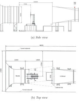
Wind Tunnel
The LLF wind tunnel used is a closed circuit, atmospheric, continuos low-speed wind tunnel. Figure 3.5 sketches the layout of the wind tunnel configuration. The wind tunnel is operated in open jet configuration throughout the MEXICO experiment. The configuration features an open test section of 9.5×9.5 m2. In this section the wind flows from a nozzle towards the collector (closed loop between nozzle and collector). The range of the upstream velocity of this tunnel is between 5.5 m/s and 30 m/s.
The blockage of the rotor model counts for 18% of the total area of the nozzle which should result in a negligible solid blockage. An open jet is used instead of a solid wall wind tunnel.
In addition to the tunnel balance data sensors were installed to measure: velocity, temperature, barometric pressure (to obtain density). In the collector entrance 8 pressures sensors were installed additionally.
(a)Side view
[image:52.595.177.447.332.677.2](b)Top view
3.5. MEASURMENTS AND INSTRUMENTATION 31
3.5
Measurments and Instrumentation
Several types of measurements were obtained during the experiment, like pressure, acceleration, temperature, moments in three directions at the root of the tower (with a 6-component balance), edgewise and flatwise bending moments at the root of the blades, strain gauges, upstream velocity, yaw angle, rotor speed, generator torque, pitch angle, and an optical 1P sensor that generated the trigger signal for the recording of the information.
The model rotor was instrumented with 148 fast Kulite® XCQ-95-062-5A pressure sensors to measure the pressure distribution over 5 sections of the blades. More specific information about the pressure sensors can be found on the Table C1 in the Appendix C. For the two directions of the bending moments, strain gauge bridges were applied at the root of the three blades. Lastly, a large number of Particle Image Velocimetry (PIV) studies were programmed to indicated tip vortices and determine near field inflow and wake velocities as well as the flow field around the rotor. From all these measurements the pressure distribution is of special interest for this work.
The pressure distributions will be used for validation of the multilevel panel method. We focus on the time dependent pressure distributions from the New MEXICO experiment to validate the multilevel panel method from [48] as these are the primary aerodynamic data. Validation of this panel method with derived quantities like lift, bending moment or torque would obfuscate the analysis as a result of the possibility of cancelling errors.
Table 3.2: Position of pressure sensors at blade and radial location
Radial location Blade Number of sensors Function
[%] # [−]
25 1 28 Measurement
35 1 27 Measurement
60 2 25 Measurement
60 1 8 Reproducibility
60 3 5 Reproducibility
82 3 25 Measurement
82 2 5 Reproducibility
92 3 25 Measurement
3.5.1 Data Acquisition
one blade. Along these measurement sensors, a limited number of extra sensors were mounted in similar locations at the other blades to check the reproducibility of the pressure measurements on different blades. The distribution of the pressure sensors according to its function is shown in the Table 3.2
3.5.2 Uncertainty of Pressure Sensors
Careful attention must be given to the pressure sensors measurements since the sensors registered absolute pressure. The pressure range of this sensors is 35 kPa. It is mentioned in [64] that the sensors a have an uncertainty of 1% of the Full Scale Output (FSO), resulting in an uncertainty of 350 Pa. The dynamic pressure is defined equal to
q = 1 2ρ
U∞2 + (ωr)2
(3.1)
This allow us to see that the difference in the pressure coefficient ∆Cp by cause of the uncertainty in the pressure sensors is
∆Cp= 350
q =
350 1
2ρ
U2
∞+ (ωr)2
(3.2)
The crucial importance of the uncertainty for the measurements and for the future comparison of the pressure distribution lies on the influence of the radial location. Is possible to see in the Table 3.3 the estimated difference in pressure coefficient related to the increase in the radial location.The influence of the uncertainty in the pressure sensors will be lower in the outer sections of the rotor, this is because the relative velocity and the dynamic pressure increase in this direction.
Table 3.3: Estimated pressure coefficient due to uncertainty in the pressure sensors at radial loca-tions forρ= 1.20421 kg/m3,U∞= 14.7 m/s and 425.1 rpm.
Radial location q ∆Cp
[%] [Pa] [−]
25 508 0.69
35 870 0.40
60 2305 0.15
82 4192 0.08
3.6. DATA SELECTION FOR VALIDATION 33
3.5.3 Measurement Data Points
During the experiment every combination of model and tunnel configuration measured corresponds to a unique data point. Nearly 1400 points of such data were recorded. The data points are organised in runs (between tunnel on and tunnel off) and polar(s). This give a unique name combination for each datapoint, the usual notation was R for run, P for polar and D for data point. Each measurement data point contains information recorded under the specific conditions of that data point. Every data point represents a recording of approximately 5 seconds3and it contains the information collected by the sensors, like pressure, RPM, pitch, wind velocity, an other parameters. It is mentioned that for the first MEXICO campaign one of the most important features of the measurements is the extensive flow field mapping by stereo PIV measurements [60]. However, this comment is not made for the New MEXICO experiment, which repeats many of the first cases for the validations of those.
A measurement data point corresponds to a recording during which the conditions remained con-stant in terms of tunnel conditions and model configuration. The exception is on the dynamic inflow measurements (for example for data points with the pitch step or rotor speed step). Is mentioned before that every data point represents a recording of approximately 5 seconds. The sampling frequency is 5524 Hz, therefore each measurement data point file is going to contain around 27500 samplings. For the dynamic cases the time interval raised to 15 s per file giving nearly 82700 samplings. For most of the cases the rotor speed was around 7.06 Hz (≈ 424 rpm). Hence, each measurement data point contains information of around 35 revolutions 4. Finally, at 7 rev/s and with the sampling frequency is possible to see that the samplings were taken approximately every 0.5◦ angular interval (see 4.1).
3.6
Data Selection for Validation
It is noted by now that the measurements covered a large combination of parameters resulting in a large number of repeated cases [60, 63, 65]. A complete table of cases and aerodynamic conditions can be found in the Table B2 in Appendix B, and for more details the reader is referred to [66]. The list of the cases used for the current work is summarised as follows:
1. Yawed rotor: The measurements have been done at rotor yaw angles −30◦, 15◦, 30◦ and
45◦. The rotor speed is kept constant at its design value of 424.1 rpm and tunnel wind speed is kept at 15 m/s. The pitch angle is kept constant at−2.3◦.
2. Dynamic inflow step in blade pitch: A blade pitch step varied from−2.3◦ to 5◦ (up and
down), while maintaining design conditions; rotor speed is kept constant at 424.1 rpm and tunnel speed of 15 m/s and axi-symmetriccally.
3
In dynamic cases the files contain information of up to 15 seconds of recording
4
7rev s ×5
s f ile = 35
![Table 1.1: A partial record of the growths and impacts of human activities during the 20th century,from [2]](https://thumb-us.123doks.com/thumbv2/123dok_us/9748547.475839/24.595.183.439.150.382/table-partial-record-growths-impacts-human-activities-century.webp)