Validity of the EDA Explorer as a means for artifact rejection and peak detection in electro dermal activity data analysis

Master

’s

Thesis

‘

Validity of the EDA-Explorer as a

means for artifact rejection and

peak detection in electro dermal

activity data-

analysis’

Jan Hemmelmann

s1367552

Faculty of Behavioral Science

Psychology

Department of Human Factors

Dr. M. L. Noordzij (Primary Supervisor)

Dr. P. M. Ten Klooster (Secondary Supervisor)

A

The recent increase in wearable technology and their application in scientific studies as well as in everyday life is calling for new ways of analyzing the data retrieved. In a psychological framework the combination of wearables with automated analysis software could make real-time biofeedback significantly more accessible to health care professionals. The Massachusetts Institute for Technology has developed the EDA-Explorer, a tool which promises to relieve the often unskilled professional from manually finding peaks and disturbances - so called artifacts - in the data sets of laboratory and ambulatory research. This study aims to validate this tool by comparing its output against the ‘golden standard’

for electrodermal activity (EDA) analysis. In a laboratory experiment, participants were asked to complete three tasks that would stress-test the Empatica E4, a measurement device for electrodermal activity. Peak detection and the artifact rejection were then performed by both the EDA-Explorer and Ledalab and Visual Inspection respectively. The EDA-Explorer’s Through-To-Peak method for identifying peaks could be shown to be accurate to the point of outperforming both Ledalab’s Through-To-Peak and

I

Abstract ... 2

Index ... 3

1. Introduction ... 5

1.1 Electrodermal Activity ... 6

1.2 Skin Conductance Response (SCR) ... 6

1.3 Problems with the analysis of EDA data ... 7

1.4 Wearable technologies and their application ... 9

1.5 Problems with wearable technologies in the realm of EDA ... 10

1.6 Artifact detection and rejection and the ‘state of the art’ ... 11

1.7 The EDA-Explorer ... 13

1.8 Scope and roadmap ... 13

1.9 Research Question & Hypothesis ... 14

2. Method and Material... 14

2.1 Data collection ... 14

2.2 Materials ... 14

2.3 Procedure ... 15

2.4 Conversion and analysis ... 17

2.5 Sample size ... 19

3 Results ... 20

3.1 Peak detection ... 20

3.2 Artifact rejection ... 24

3.3 A systematic error report on the usability of the Empatica E4 ... 28

3.3.1 Failure of creating a proper EDA signal ... 28

3.3.2 Failure of export... 30

4.1 Answer to the hypotheses ... 33

4.2 Discuss findings in light of Alternative tooling ... 34

4.3 Limitations ... 36

4.4 Practical implications ... 37

5. References ... 39

6. Appendix ... 41

Appendix 1 – Instruction for the participant ... 41

Appendix 2 - Informed Consent ... 41

Appendix 3 – Data set conversion... 43

Appendix 4 – Data, scripts, graphs & more... 57

1.

I

Accelerated progress in recent years in the realm of wearable technology has opened up novel opportunities for ambulatory studies concerned with human physiology. Nowadays, wearable sensors such as the Empatica E4 are enabling researchers to gain a unique insight into the emotional state of a participant or client at any given point in time and place (Callaway & Rozar, 2015; Mukhopadhyay, 2015). Specifically, the measurement of electro dermal activity (EDA), which is retrieved from measuring the skin conductance level (SCL) on the human skin, has for many years found use cases in applied research, psychotherapy and the evaluation and treatment of schizophrenia, depression and anxiety (Venables, 1977). From a psychological framework this cross between physiological measurements and portability introduces many new possibilities (such as longitudinal studies and real-time real-world monitoring) as well as challenges (such as disturbances and the amount of data produced) (Erçelebi, 2004; Kitipawang, Kakria, & Tripathi, 2015a; Taylor et al., 2015; Zhang, Haghdan, & Xu, 2017). The goal of this paper is to address these challenges and evaluate a technical solution designed to overcome them.

Recently, the Massachusetts Institute of Technology published the first automatic artifact rejection tool for electrodermal activity data. This analysis tool is called the EDA-Explorer (Taylor et al., 2017). The measurement of EDA-data over a long period of time in ambulatory scenarios generates a considerable amount of noise, also called artifacts. Visual inspection by a human analyzer is the ‘state of the art method’ for dealing with such

1.1

E

A

Electrodermal activity or EDA can be described as autonomic, electrical variations on the surface of the human skin. Such variations can be caused by stressors, an increase or decrease in temperature (Wenger, 2003), or physical or mental efforts (such as running or mental problem solving), which lead to the perturbation of the ongoing regulatory activities of the sympathetic nervous system (SNS) (Dawson, Schell, Filion, & Berntson, 2015). The SNS causes a stimulation of the body’s sweat glands, also called sudomotor innervation. The result is perspiration and it is responsible for the electrical variations as mentioned above, which can be measured non-intrusively (Boucsein et al., 2012) and quantified by placing two electrodes apart from each other onto the skin and applying a small voltage. What is measured is the called Skin Conductance (SC), which in a general sense can be related to emotional arousal (Boucsein, 2012), which makes SC data an interesting source of information in a clinical setting as well as in other fields of research. The unit of measurement is MicroSiemens (μS). General SC can be divided into the underlying Tonic

Skin Conductance Level (SCL) and more rapid, Phasic Skin Conductance Responses (SCRs). SCL can be better understood as the level of skin conductance that is specific to the individual. It can be estimated by measuring a time interval of rest. SCRs are responses to external or internal stimuli, such as a sudden loud noise or disturbing thoughts, that cause sudomotor innervation by the SNS.

1.2

S

C

R

(SCR)

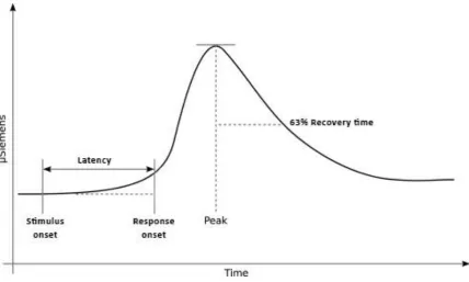
FIGURE 1 – A TYPICAL SKIN CONDUCTANCE RESPONSE

As described in Figure 1, a SCR can follow shortly after a certain stimulus (such as a sudden loud noise). The time between stimulus onset and response onset is described as latency and lasts for roughly 1-5 seconds (Boucsein, 2012.; iMotions, 2016). After a quick rise time, the signal reaches its peak which appears at the moment where the SCR arrives on its highest amplitude. After the peak, the amplitude slowly returns to its original state. The time of this process is also called recovery time. In a stressful situation, SCRs can occur frequently and sometimes quickly after one another (Macefield & Wallin, 1996). In such a case, superposition of SCRs occurs, when the next SCR starts before the last one had time to fully recover.

1.3

P

EDA

First, SCRs never start at zero. As mentioned before, every person also has a different SCL depending on for example their skin type, or the temperature in the lab, meaning that the SCRs in which the researcher might be interested in start from this specific tonic amplitude. In order to come to a valid estimation of the onset and amplitude of a single response, SCL needs to be taken into account.

Second, superposition or the stacking up of SCRs before the signal has fully recovered to its original state is a prominent research topic because it holds the potential of contaminating the data set, which can result in researchers and clinical staff to come to wrong assumptions about certain responses. Neglecting the effect of superposition, would frequently result in an underestimation of the amplitude of the following SCRs (Benedek & Kaernbach, 2010). Commonly, the through-to-peak or TTP method is used for peak detection. However, TTP does not account for superposition, which occurs when a new SCR starts while the relaxation periode of the previous SCR has not yet finished. In order to achieve a proper estimation of amplitude, research identifies methods for correcting the effects of superposition. The decomposition method by means of deconvolution was one of the first attempts to get closer to the ‘real’ skin conductance level by estimating the

and extended by the Continuous Decomposition Analysis (CDA), which now serves as the golden standard for peak detection in EDA data.

Analysis tools for electro dermal activity implement computer algorithms that automatically (but progressively time consuming with the length of the data set) calculate amplitudes according to the knowledge about superposition. A frequently used analysis tool for peak detection in EDA data is Ledalab. CDA is accessible via the Ledalab software (“Ledalab Software,” 2016). For the purpose of this study and because of its wide

application and years of research and intensive documentation, LEDALAB is considered the golden standard for peak detection. It should be noted though, that research should never solely rely on automated tooling. A visual inspection of the data set should always be performed in order to further support the results retrieved from automated tooling.

1.4

W

In recent years wearable technologies have started spreading greatly into everyday life. The measurement of heart rate, footsteps and calorie burn has become drastically easier because of wearables, but also a wide variety of informational services recently experienced a shift from the smart phone to the smart watch (“Apple Smart Watch,” 2018; “Fitbit Smart Watches,” 2018; “IDC Tracker® + Data Products,” 2018; “Samsung Smart

Watches,” 2018). But the use cases are not restricted to the private sector. The Empatica E4

The development of wearable technology contributes to a shift from controlled lab studies to ambulatory, real-time and real-world measurements (Goodwin, Velicer, & Intille, 2008). In an even broader context, wearable technology is already being used for continuous medical monitoring for patients that would otherwise need to be hospitalized (Edwards, 2012). In such cases the technology offers real time monitoring and feedback, as well as long term statistics of wellbeing to the individual, the doctor and even friends and family (Kitipawang, Kakria, & Tripathi, 2015b; Salvo, Francesco, & Costanzo, 2010). While the technology holds great potential to gather unique data, the real-world environment can compromise the collected data sets.

1.5

P

EDA

The real world is uncontrollable, and so are the occurrences that people encounter every day. The unpredictable nature of events creates new challenges for researchers when using wearable technologies for their research, especially when it comes to EDA data. Distinguishing the cause of specific SCRs is one problem. As described above, SCRs can result from a variety of different stimuli. Even more problematic is the distinction between an SCR and a so-called artifact.

creating pressure on the sensor of the measurement device or moving his/her arm so fast, that the placement of the sensor on the arm shifts. This disturbance might not even trigger the SNS of the participant (and is therefore unrelated to any bodily functions), but it certainly creates an artifact on the data set, which could then later be confused with a normal SCR and could therefore be misleading in the interpretation of the data. The first category of artifacts (motion of the body) lies outside the scope of this paper as this research identifies ambulatory longitudinal studies to be the great benefit of wearable technology. In such studies, the first category of artifacts is not only a constant given but can even be valuable information to the researchers. Furthermore, those kinds of artifacts can not be categorized because they can not be distinguished visually from normal SCR’s.

This research focuses on the second category of articats, external disturbances (or the movement of and pressure on the sensor of the measurement device) only. From this point onward, those kinds of disturbences are meant when the term ’artifact’ is used.

Artifacts can differ in nature. Literature most prominently addresses motion artifacts which arise from the movement of the limb that the measurement device is attached to (Chen et al., 2013; Zhang et al., 2017). Similar to the one created by motion, pressure on the measurement device can also create artifacts, so called pressure artifacts (Edelberg, 1967; Xia, Jaques, Taylor, Fedor, & Picard, 2015). Pressure artifacts can be described as external pressure or even muscular activity that increases the pressure on the wristband for a short period of time and thereby disturbing the signal. Both kinds of peaks can look similar to a normal SCR on the data set and are likely to appear in ambulatory longitudinal studies but add no potential value to the topic of interest and can even be harmful to the analysis process when gone unnoticed.

1.6

A

‘

’

prevent them as much as possible (Braithwaite, Watson, Jones, & Rowe, 2013). However, even when introduced properly artifacts will eventually appear on a data set that has been recorded over a longer period of time. The first step towards Artifact rejection is artifact identification. Boucsein (1992) states:

“The detection of artifacts in the EDA signal necessitates a visual inspection of the data

sequence by the experimenter, even if an automatic parameterization is performed by

means of laboratory computers”

He further proposes that artifacts should already be detected during the experiment (Boucsein, 2012). Today, 25 years later, the application for EDA measurements has spread so far into the realm of wearable technology and away from controlled lab studies, that a manual detection during those types of recording is not feasible any longer due to the sheer amount of data recorded in just a few days. Also, a later evaluation of those kinds of data set becomes challenging for the same reason.

1.7

T

EDA-E

The EDA-Explorer is a tool programmed in Python (version 2.7) that promises to automatically run over the entire data set and identify both peaks and artifacts. Taylor et al.’s (2017) approach for artifact rejection was to train the Explorer using the Support

Vector Machines machine learning algorithm. The Explorer was trained by EDA experts who judged 1560 five-second intervals as either clean, questionable or containing artifacts. It should be noted that the researchers are not making a distinction between motion and pressure artifacts. Less information is provided about their approach for Peak detection. The script does not use the CDA standard that is handled by LEDALAB but relies on more rudimentary TTP analysis where first- and second-order deriviates of the SC signal are evaluated for speed and acceleration changes typically found when an SCR occurs. Another limitation of the EDA-Explorer is that it can only process one raw file at a time. Therefore, working with multiple data sets in the online solution or the downloaded Python script can become time consuming. In the study at hand, the EDA Explorer was used in combination with a batch script developed by Matthijs Noordzij and Peter de Looff (provided on request) which allowed for the processing of multiple (without limit) E4 files of multiple subjects automatically.

1.8

S

The Scope of this paper is to judge the validity of the EDA-Explorer as a measurement tool for ambulatory EDA data. This is done by exploring the similarities and differences between the EDA-Explorer and the golden standard for both peak detection and artifact rejection. The emphasis of this paper lies on longitudinal real-world studies with the Empatica E4. Generalizability to other scenarios is limited and will be further debated in the discussion section.

1.9

R

Q

&

H

To what extent does the judgment of an artifact-rich dataset by Visual Inspection and Ledalab agree or disagree with the judgment concerning artifact rejection and peak detection performed by the EDA-Explorer? As an answer to the research question this study proposes two general hypotheses. The first hypothesis addresses peak detection. The later hypothesis addresses artifact rejection.

Hypothesis 1: The agreement in the number of peaks per time interval and moment of peaks between the EDA-Explorer (TTP) and Ledalab (TTP) is visually clearly detectable.

Hypothesis 2: The agreement in the number of artifacts and moment of artifacts per time interval between the EDA-Explorer (binary and multiclass) and Visual Inspection is visually clearly detectable.

2.

M

M

2.1

D

20 participants, 14 male and 6 female students, between 22 and 29 years of age, participated in the experiment. The location for the experiment was the lab rooms on the University grounds and the staircases surrounding it. The procedure was the same for every participant. The experiment was approved by the ethical commission of the University of Twente prior to execution. All participants signed an informed conset prior to the study (see Appendix 2). No participants received any rewards for their participation. A pre-test was performed with two students at the age of 24 and 25 in order to get an insight into the effectiveness of the tasks in evoking artifact rich data.

2.2

M

acceleration in three axes at 32 Hz and temperature on the skin at 4 Hz (“E4 wristband technical specifications,” 2016a). The participant was seated in a normal, upright sitting

position in an office chair in the lab room. All participants were informed about the nature of the study (see Appendix 1). All instructions were given verbally. All data was processed via the Empatica online service and anonymously saved on the computer of the researcher for further analysis.

2.3

P

For every participant, the experiment took 25 minutes. The first 10 minutes were used to verbally introduce the participant to the experiment and explain every task he/she was about to perform. The participant was also introduced to the functionality of the Empatica E4 and questions were answered. The participant was asked to walk up and down a flight of stairs prior to the experiment to assure a minimum level of perspiration and thereby a clean measurement as is reccomended by Empatica (“E4 wristband technical specifications,” 2016b). The E4 wristband was put on the dominant hand of the participant

bag weighed 5kgs. No specific instructions on how to carry the bag were given. The last task was to play rock-paper-scissors (RPS) with the researcher, whereby operationalizing heavy movement and probably the misplacement of the watch on the participants arm. The artifacts created by the RPS task were expected to (1) stress test the E4 and (2) vary in intensity depending on how engaged the person was playing the game. Scores of the game were not recorded. Lastly, the participant was debriefed, and the E4 turned off and removed. The data from the E4 was uploaded and then downloaded onto the researcher’s computer via the Empatica Manager. The device was then cleaned for the next participant. It was also made sure that the battery was properly charged at all times in order to avoid electrical artifacts. The internal time of the E4 was synced with the researcher’s laptop. This laptop also served as a timer for the experiment.

2.4

C

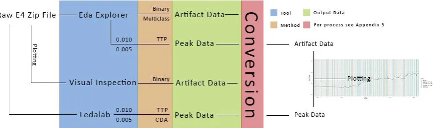
FIGURE 2 - ANALYSIS ROADMAP FROM RAW E4 OUTPUT FILE TO PLOTTING BOTH ARTIFACT REJECTION AND PEAK DETECTION DATA.

EACH DATA SET WAS ANALYZED BY ALL METHODS OF EACH TOOL. ARTIFACT- AND PEAK-DATA FROM THE EXPLORER WERE THEN

CONVERTED INTO THE SAME FORMAT TO ALLOW FOR COMPARISON.

The data analysis was done in multiple steps as illustrated above. After savind the raw file from the E4 to a dedicated location on the researcher’s laptop, all data sets were

first automatically extracted, analyzed and then exported into artifact and peak data by the EDA-Explorer. The artifact data was created by the binary method, which classifies every five second interval as either (-1) containing an artifact or (1) containing no artifact and the multiclass method, which classifies every five second interval as either (-1) containing and artifact, (1) containing no artifact or (0) uncertainty. The peak data was created by the TTP method using a threshold (or sensitivity) of 0.01 μS changes and 0.005 μS changes. This means that the EDA-Explorer created four data sets, two artifact data sets and two peak data sets.

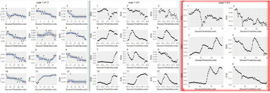
FIGURE 3 - PLOTTING DECISION FROM LEFT TO RIGHT (5 SECOND INTERVAL WITH DOTS AND MEAN SCORE WERE FOUND TO BE INSUFICIENT FOR AN ACCURATE JUDGEMENT SINCE THEY PROVIDE TOO LITTLE CONTEXT. 10 SECOND INTERVALS AND DOTS WERE OFFERING SOMEHWAT MORE CONTEXT. THE FINAL DECISION WAS TO USE 15 SECOND INTERVALS AND LINES IN ADDITION TO THE DOTS FOR MAXIMUM CONTEXT WITHOUT LOSING TOO MUCH DETAIL)

Figure 3 shows the visual differences in plotting various time intervals. While choosing an appropriate time frame, scale and visualization, it became apparent that the context (or the five seconds before and after the to be rated five second interval) could be an important asset for arriving at an accurate rating. This context may be useful for the rating since artifacts can be compared to and therefore distinguished from SCR’s and artifacts may also be occuring in between two intervals. In those cases, raters were instructed to classify both intervals as containing artifacts. Furthermore, fifteen second intervals do not yet lack the detail that is crucial when it comes to identifying the shape of the peak. Additionally, it was chosen to use a combination of lines and dots for better readability. Once the plots were created, the visual inspection was performed by two raters using the visual inspection method. Both raters were students who were trained using the LEDALAB paper on SCRs and Taylor et al’s paper on artifact rejection (Benedek, 2011; Taylor et al., 2017). The rating was

Thirdly, LEDALAB was used to perform the peak detection using the same threshold values as the EDA-Explorer (0.005 and 0.010 μS). From LEDALAB the TTP and the CDA methods were used for both thresholds resulting in four data sets.

In this manner each raw E4 zip file created nine output data sets (three for artifact rejection and six for peak detection). Before comparing the different outputs to each other, some of the data sets had to be converted in order to match the data structure. For example, Ledalab uses the time from onset of the measurement device, whereas the EDA-Explorer uses the Unix time stamp as a measurement for time. In this case, it was chosen to convert the Unix time stamp into time from onset by subtracting the start time from every single measurement point (See Appendix 3 for a detailed description of this process). Peaks also had to be matched, because the EDA-Explorer identifies the actual peaks, whereas Ledalab identifies the peak’s onset. The EDA-Explorer output was therefore adjusted in order to also identify the peak’s onset. The converted data was transferred to .csv and SPSS files which in turn served as the foundation of all analyses.

Lastly, the data sets of all participants were plotted using an R-script that was developed by the researcher (See Appendix 3). The plotted data was then visually examined for peaks and artifacts. All statistical analyses and their results can be found in the results section below.

2.5

S

3

R

The below results were devided into two major parts. The first part concerned peak detection and the second part concerned artifact rejection. A third part was added in order to systematically report all errors that were encountered during the experiment (which led to the exclusion of many participants) in order to inform future research about possible problems with the use of the measurement device.

3.1 Peak

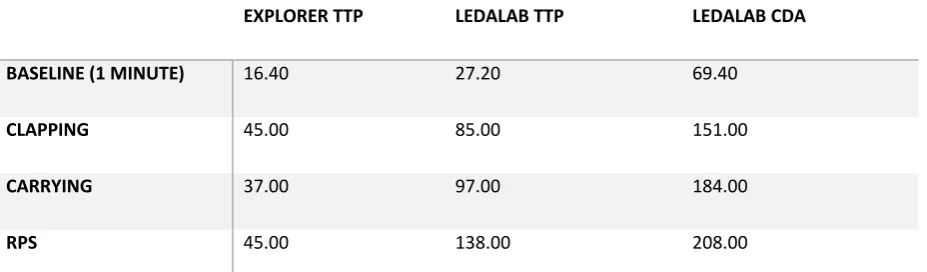
The peak detection was run by both the EDA-Explorer and Ledalab (using TTP and CDA method) for two thresholds (.005 & .010). The analysis revealed that there is only a slight difference between the two thresholds. Both .005 and .010 measurements could be used interchangeably, because they consistently identified the same points in time as peaks. A .005 threshold identified slightly more peaks than the .010 threshold (see Appendix 5). Furthermore, it can be shown (as could be expected from literature) that the Ledalab CDA method is more sensitive of a method for peak detection than TTP. Ledalab CDA identifies an average of N=153.1 peaks per data set, whereas Ledalab TTP identifies N=86.8 and Explorer TTP only N=35.85 peaks.

TABLE 1 - SUM FREQUENCIES SUMMARIZED FOR ALL FOUR PARTICIPANTS DEVIDED BY TASK AND ANALYSIS METHOD

EXPLORER TTP LEDALAB TTP LEDALAB CDA

BASELINE (1 MINUTE) 16.40 27.20 69.40

CLAPPING 45.00 85.00 151.00

CARRYING 37.00 97.00 184.00

RPS 45.00 138.00 208.00

because the duration of the entire experiment was 11 minutes. For the peak detection it was chosen to compare the means of peaks found in this specific time interval. Calculating Cohens Kappa revealed no agreement between any of the three methods. All scores are listed in the table below.

TABLE 2 - INTER-RATER AGREEMENT BETWEEN EXPLORER TTP, LEDALAB TTP AND LEDALAB CDA

AGREEMENT BETWEEN… N KAPPA SIGN.

LEDALAB CDA AND EXPLORER TTP 22 0.00 NAN LEDALAB TTP AND EXPLORER TTP 22 -0.004 0.746, LEDALAB TTP AND LEDALAB CDA 22 -0.10 0.608

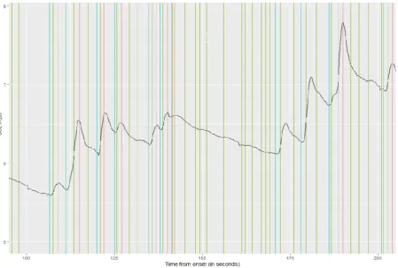
The graph below contrasts Ledalab’s CDA, TTP and the Explorers TTP method on one representative sample data set.

FIGURE 4 –LEDALAB’S CDA METHOD IS TOO SENSITIVE BECAUSE IT IDENTIFIES MANY PEAKS IN A CLEAR RELAXATION PERIODE

experiment. During this time, there was little change in SCL, yet the CDA method identified a total of 10 SCR’s during that time interval. This sample was just one representative example of many. Another finding that could be displayed in the graph above is that the EDA-Explorer identified the top of the peaks whereas Ledalab set the point of peak identification at the beginning of the SCR (as mentioned in the method section and see Appendix 5). The CDA method identified the halfway point between onset and actual peak. This is due to the fact that CDA makes an attempt of calculating the underlying sudomotor activity rather than simply finding the peaks on the graph. These differences were accounted for in the further calculations.

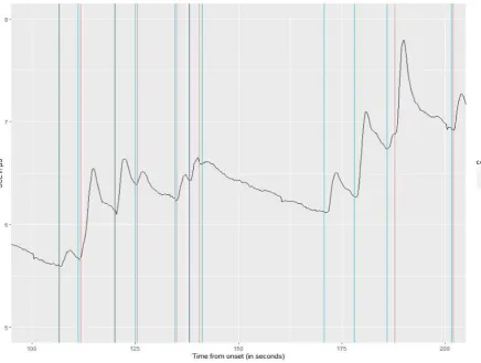
FIGURE 5 - ADJUSTED EXPLORER TTP METHOD SHOWS CLOSE SIMILARITY WITH LEDALAB'S TTP METHOD, BUT THE EXPLORER TTP METHOD MISSES TWO SCR’S.

which the EDA-Explorer fails to identify two of the SCR’s as peaks. Interestingly, the greatest difference between the EDA-Explorer’s peak detection and Ledalab’s peak detection is, that the Explorer accurately negated most artifacts as peaks, whereas Ledalab’s TTP (and CDA) methods also rendered artifacts as peaks. This is further explored in the graph below.

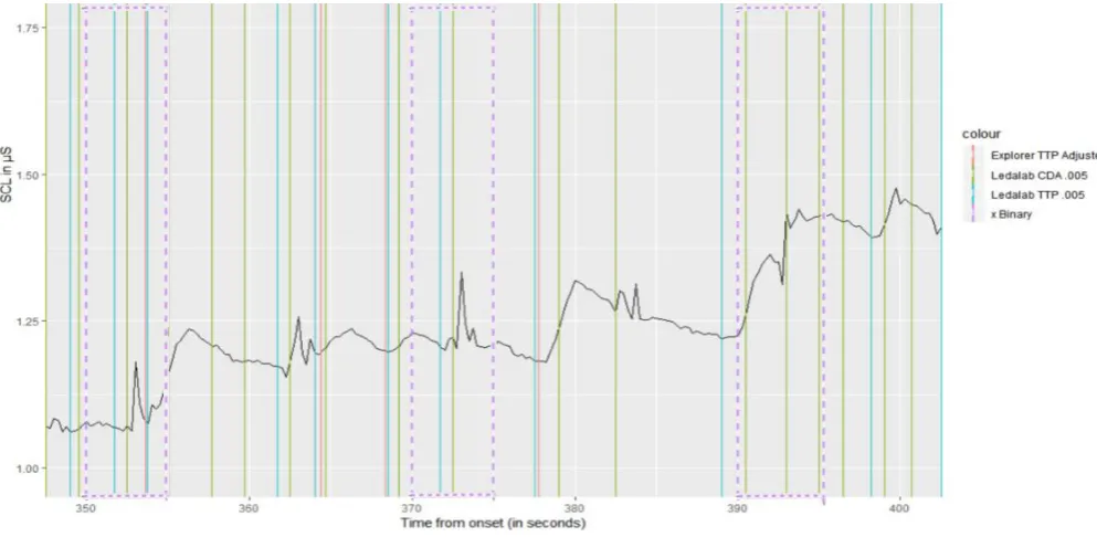
FIGURE 6 – THE EDA-EXPLORER SEEMS TO IGNORE ARTIFACTS IN THE PEAK DETECTION. THE BINARY METHOD IDENTIFIES MOST BUT NOT ALL OF THE ARTIFACTS. NOTE THAT THE EXPLORER'S BINARY METHOD RENDERS FIVE-SECOND INTERVALS AS CONTAINING ARTIFACTS OR NOT (THE DOTTED LINES).

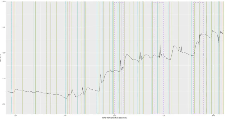
FIGURE 7 - BASELINE 40-340 SECONDS, CLAPPING TASK 340-460 SECONDS, START OF CARRYING TASK 460 SECONDS. BINARY METHOD VISUALIZED AS FIVE SECOND INTERVALS. MULTICLASS ARTIFACT REJECTION DOES NOT IDENTFY ANY ARTIFACTS IN THE CHOSEN INTERVAL.

Visually it was relatively easy to identify a pattern of artifacts followed by a SCR, followed by another artifact and then another SCR. Interestingly, every ‘spiky’ peak (the artifact) was followed by a SCR. This SCR could, as we addressed in the introduction, be classified as an artifact of the first category (one which is produced by the SNS as a reaction to a trigger that was not intended by the researcher). The current research was not interested in these kinds of artifacts. Strangely, the EDA-Explorer rendered most of these aretifacts as neither peak nor artifact, but simply ignored the occurrence. An interaction between the EDA-Explorer’s peak detection and artifact rejection method was tested for by running all methods first separately and then combined. Both ways of analyzing produced the exact same results. An interaction between the methods can therefore be ruled out as an explanation for this phenomenon.

3.2

A

algorithm can only accidentally fall right on the artifact when that artifact occurs right at the beginning of the time interval. The dotted lines for all plots that follow indicate the starting point from which the five second interval starts. It was chosen for this, because plotting artifacts as intervals make the plots unreadable.

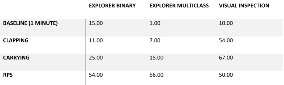
Diving into the data revealed some major findings about the artifact rejection algorithms. To begin with it could be shown that the binary method identified more artifacts than the multiclass method did, even when including all ‘uncertain’ (represented by 0 values in the data set) identifications of the multiclass method. On average across all four experiments the Explorer Binary method found N = 26.25 artifacts, the EDA-Explorer Multiclass method found N = 19.75 (N = 55 including uncertainty) and Visual Inspection found N = 52.75 artifacts.

TABLE 3 - SUM FREQUENCIES SUMMARIZED FOR ALL FOUR PARTICIPANTS DEVIDED BY TASK AND ANALYSIS METHOD

EXPLORER BINARY EXPLORER MULTICLASS VISUAL INSPECTION

BASELINE (1 MINUTE) 15.00 1.00 10.00

CLAPPING 11.00 7.00 54.00

CARRYING 25.00 15.00 67.00

RPS 54.00 56.00 50.00

TABLE 4 - INTER-RATER AGREEMENT BETWEEN BINARY, MULTICLASS AND VISUAL INSPECTION

AGREEMENT BETWEEN… N KAPPA SIGN.

BINARY & MULTICLASS 22 0.351 0.000

BINARY & VI 22 0.138 0.017

MULTICLASS & VI 22 -0.127 0.080

FIGURE 8 - ARTIFACT REJECTION BINARY, MULTICLASS AND VISUAL INSPECTION ACROSS THE ENTIRE TIME SPAN OF THE EXPERIMENT

FIGURE 9 - VISUAL INSPECTION VS EDA-EXPLORER BINARY AND MULTICLASS DURING THE CLAPPING TASK. NOTE THAT EACH LINE INDICATES THE STARTING POINT OF A FIVE SECOND INTERVAL.

FIGURE 10 - VISUAL INSPECTION VS EDA-EXPLORER BINARY AND MULTICLASS DURING RPS TASK

The experiment was set up to make the last task the most artifact heavy task. This can be found back in all data sets. For this task, the binary method identified almost every single five second interval as containing artifacts, whereas visual inspection suggested that artifacts only occur heavily in the beginning of the task. The multiclass method identified different intervals than visual inspection and the Explorer binary method.

All of the above statements were double checked with (1) different time intervals within the same data set, (2) the same intervals in different data sets and (3) other time intervals in other data sets. All findings were consistent with the findings presented above. (also see Appendix 5)

3.3

A

E

E4

Of all 22 datasets, only 4 could be used for the analysis. 18 data sets had to be rejected. The various causes for the rejection of those data sets gave reason to have a closer look at the Empatica E4 and what went wrong in the experiment. This part of the paper specifically focuses on systematically reporting all problems with the E4 and the experimental design and to make suggestions for their improvement.

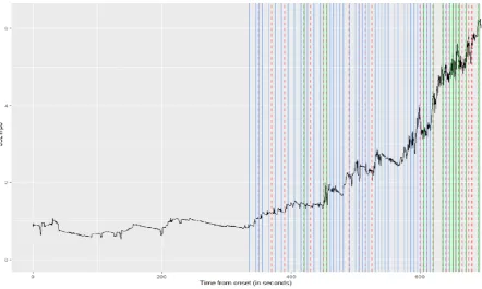
FIGURE 11 - DESCRIBES THE SCL LEVEL OF SESSION 6. A LOW SCL DURING BASELINE, CLAPPING TASK AND CARRYING TASK AND A

SUDDEN INCREASE IN SCL IN TASK 3 CAN BE NOTED.

The problem with most measurements, as can be seen in Figure 8, was that almost no signal was picked up during the first half or even the entire time of the experiment. Given such a signal it was impossible for the EDA-Explorer or Ledalab to identify any peaks or artifacts. Seeing the figure above, it could also be ruled out that the E4 was compressing the signal in any way. What appears most likely in this case is that the sensor did not pick up a signal because of a wrong placement of the wristband on the wrist. Personally, I assume that the E4 was applied too tightly on the skin preventing the sweat glands from releasing water or the sweat being able to form a continuous layer on the skin. Suddenly, the arm was moved so abruptly, that the wristband was slightly relocated and picked up a signal from the surrounding glands that were able to release water the whole time, causing an increase in SCL. Another possible explanation could be that the E4 only recorded a signal from a certain threshold and the participant was not sweating enough.

participants. Therefore, in the following round of experiments, for 10 participants, the warm up phase was adjusted. The participants were asked to walk up and down a flight of stairs five times and were noticeably breathing more heavily right before starting the experiment. Yet, 3 out of 10 data sets had to be discarded again because of an unusable SCL. The most apparent problem with inducing perspiration in the first place is it raises the baseline SCL, which if not consciously accounted for can possibly influence the results of other experiments. A balancing act must be performed between too much or too little warm up, which in both cases would render the data set useless. In this context, an additional problem occurs. When it comes to longitudinal measurements, the experimenter has no live feedback when using the E4 in its standard recording mode. That means that the researcher has no choice but to (1) do a pre-test via Bluetooth mode or (2) check the data set daily after upload. Suggestions for improvement include (1) a more sensitive sensor or higher amplitude, (2) the LED indicating when SCL drops below 1.25μS (which was found to be the minimum value in valid data sets from this experiment) and (3) allowing live feedback via Bluetooth connection while data is recorded to the hard drive of the E4.

3.3.2 FAILURE OF EXPORT

allows the user to manually skip the down- and upload of a specific file or (2) a software update that allows the user to directly access the hard drive of the E4.

3.3.3 USABILITY ISSUES

A few usability issues were discovered throughout the experimental phase. Firstly, almost all participants needed help with putting on the wristband in the first place. Furthermore, it often happened that the wristband needed adjustment after closing it because it was either too tight and therefore uncomfortable, or too loose for a proper recording of EDA data. A possible solution would be to redesign the closing mechanism of the wristband as shown in Figure 9 and 10 below. Figure 9 shows a wristband that goes through a slope on one side of the watch and then returns to the middle where it is possibly held by a magnet. The magnet here could possibly interefere with the skin conductance electrodes. Figure 10 shows another possible closing mechanism that resembles the one of a zip tie. Either closing mechanism would allow for smooth progressive and stepless adjustment for any kind of wrist.

FIGURE 13 - POSSIBLE CLOSING MECHANISM (2)

As described above, one concern with the E4 was the closing mechanism of the wrist strap. Another one was the size and appearance of the E4. It was frequently mentioned in the conversation with the participants. ¼ of all participants made a comment about the appearance of the watch, most of them reffering to its ‘clunkiness’. Similar findings were

also noted by (van Lier et al., 2017).

4

D

The discussion section is divided into four parts, starting with relating the findings back to the hypotheses and answering the research question. Part two contrasts the findings of this study with additional literature, theories and other measurement tools. Part three examines the limitations and places this research into a broader context. Finally, part four reviews the practical relevance of the findings from a psychological point of view.

4.1

A

The validity of the EDA-Explorer based on the findings from this study indicates that the peak detection TTP method performs unexpectedly well in artifact rich situations, up to the point of outperforming Ledalab’s TTP and CDA methods, whereas artifact rejection performance is varying per method and nature of the disturbance, but poor throughout.

Hypothesis 1: “The agreement in the number of peaks per time interval and moment of peaks between the EDA-Explorer (TTP) and Ledalab (TTP) is visually clearly detectable.”

Hypothesis 2: “The agreement in the number of artifacts and moment of artifacts per time interval between the EDA-Explorer (binary and multiclass) and Visual Inspection is

visually clearly detectable.” Hypothesis 2 must be rejected. It appears that both artifact rejection methods from the EDA-Explorer greatly disagree with Visual Inspection, as implemented in the present study, as they are either too sensitive, too insensitive or inaccurate depending on the task. Results indicate that the binary method on the one hand identifies many of the same peaks as Visual Inspection, but it also overestimates the amount of artifacts in artifact rich situations such as the RPS-task and underestimates the amount of peaks in artifact poor situations such as the clapping task. The multiclass method on the other hand identifies a smaller amount of artifacts than peak detection and is highly inaccurate in artifact rich situations. In artifact poor situations, the multiclass method barely identifies any artifacts. The difference between the methods is further supported statistically through no inter-rater agreement.

All of the findings can be explained by multiple factors. The first factor, as discussed above, is the frequency in which artifacts are occuring. The second factor is possibly the nature of the task itself. The RPS-Task can be described as artifact rich, given the constant

movement of the participants arm, but the artifacts created by this task can also be classified as motion artifacts. In comparison, the clapping task involves a mixture of motion and pressure. Given this distinction one might argue that both methods (binary and

multiclass) are more sensitive to motion artifacts than they are to pressure artifacts. This assumption is compatible with the notion of the multiclass method being inaccurate. However, there is only small support from the carrying task (a task specifically designed to create pressure artifacts) and there is too little research done on the EDA-Explorer as of today. Another problem with the artifact rejection approach in general could have influenced the results. Recent literature discusses the limitations of the sectioning approach by Taylor et. al’s (2017) and offers an explanation to the here observed phenomenon

(Kleckner et al., 2017) (This will be further explained and discussed in 4.2).

Most tooling (e.g. Ledalab, PsPM, Movisens Data Analyser) provide visual insight into the data sets, appliy basic filtering and identify SCRs (Bach, 2014; Joffily, 2012; Rothman & Silver, 2018; Storm, Fremming, Odegaard, Martinsen, & Morkrid, 2000). Few tools attempt to automatically detect artifacts in the data set or more specifically motion and pressure artifacts that are caused not by the recording method itself but external factors. Kelsey et. al (2017) propose a different approach to artifact detection: a single analysis for both peak detection and artifact rejection. They critique Taylor et. al (2017) because they section the data into smaller chunks. Kelsey et. al (2017) argue that peaks and artifacts are inseparable and sectioning the data may cause SCRs to be missed when they fall on the splitting point. Another issue is that, if both artifacts and SCRs occur in the same section, they cannot be properly distinguished. This insight, when relating it back to this research, offers an answer to the question why the EDA-Explorer correctly identified SCRs during the clapping task while artifact rejection missed almost all of the artifacts. It could be shown that each artifact (the clap) is almost directly followed by a SCR. The body reacts to the clap with a physiological response. This means that we can be certain of the simultaneous occurance of both artifact and SCR in the same time frame, which most likely fall into the same five-second section that the EDA-Explorer handles. Kelsey et. al’s parse recovery algorithm or orthogonal matching pursuit (OMP) offer a solution to this problem but is still being developed. Testing the data sets of this study with the novel parse recover algorithm falls out of the scope of this paper, but according to the researchers, it currently identifies peaks and artifacts with a success rate of 80%.

Kleckner et. al’s (2017) EDAQA is another open source EDA evaluation tool

designed for ambulatory EDA data analysis. Their approach features four simple rules for classifying an artifact as such: “1. EDA is out of range (not within 0.05-60 μS) 2. EDA changes too quickly (faster than ±10 μS/sec)3. Temperature is out of range (not within 30-

40ºC)4. EDA data are surrounding (within 5 sec of) invalid portions according to rules

human’s rating to the tool’s rating, unsurprisingly finding an extraordinary agreement. It can be argued that an artifact can be much more than the four-rule definition covers. In this research and with data sets that were designed to contain plenty of artifacts, handleing such a definition would have led to identifying close to no artifacts overall.

Their study is also a response to the Explorer. Their critique on the EDA-Explorer is the lack of transparency: “Although sophisticated, the authors did not indicate what rules the machine learning model used to identify any portion of EDA data as “valid”

or “invalid” based on a complex 14- dimensional EDA feature space.“ (Kleckner et al., 2017). Agreeably, this is a big limitation to their research because it makes it impossible to argue for or against their approach.

4.3

L

The population of this study is limited to students between the age of 25 and 29, whereby rendering the results more applicable to this agegroup, since people of different age groups have very different Skin Conductance Levels. It could be that older people would have created stronger or weaker peaks and artifacts on the data set which in turn could result in a different result from the analysis by the EDA-Explorer and Ledalab. Another limitation is the use of the Empatica E4. On the one hand the use of the E4 limits the generalizability of the findings to data set retrieved by other measurement devices, but more importantly it limits the overall sample size, due to its failure. The consequences of that error have severely filtered the sample to very specific data sets that are not as representative as a random selection would have been. For example, the age group has been limited to 25 to 29-year-old students. However, this limitation must also be put into perspective, seeing that the study is not interested in comparing people or groups of people to each other, but to identify the similarities and differences in analysis tools that were given the same exact data sets to analyze. The research relied mostly on visual inspection of close-up data sets and single data points.

experimental design is not an everyday life situation and even though ambulatory longitudinal studies will have to deal with similar sorts of artifacts, those artifacts will not appear so frequent or intense. This research more fundamentally gives answer to the validity of the EDA-Explorer in artifact rich situations.

4.4

P

The real value of automatic analysis tools such as the Empatica E4 lie in the field of longitudinal studies, because of the amount of time it would take to go through the data manually. Therefore, it is chosen to summarize the practical implications on the background of conducting such studies.

All findings must be seen in context. This study was really stressful for both the E4 and the EDA-Explorer. Such artifact rich measurements are not usual in everyday life situation. But even when stress-testing the E4, the EDA-Explorer is a great tool for peak detection. It is the conclusion of this research that the EDA-Explorer should be preffered over Ledalab, especially when handling artefact rich data sets. The EDA-Explorer’s ability to distingish between peaks and artifacts makes it superior in peak detection.

That said, this study also gives a good indication of the limitations for future studies that other researchers might want to consider before conducting their own experiments. For example, it is not recommended to use the Empatica E4 in cases of very low expected arousal of the SNS. Those kinds of studies should turn to stationary devices such as the Q Sensor instead. Another limitation to consider is the accuracy of artifact rejection tooling. Measuring sports activities for example might produce too many artifacts, whereby rendering the data sets useless to the researcher interested in peaks. of the EDA-Explorer’s peak detection and artifact rejection methods.

applies (2) not transparently enough documented and (3) performs greatly inaccurate in artefact rich data sets. It is the recommendation of this paper to not rely on this tool for artefact rejection in ambulatory studies in which motion or pressure artifacts (which are not produced by bodily functions, but by external events) are likely to occur paired together with SCRs. The EDAQA offers an alternative to the EDA-Explorer but oversimplifies the definition of what an artefact can be, whereby making it too insensitive (Kleckner et al., 2017). It is the opinion of the researcher that in most use cases it would be more harmful for the research to miss artifacts, than it would be to identify too many measurement points as artifacts, since the real value of longitudinal EDA data usually lies in the occurance or absence of SCRs. However, this must be considered individually by other researchers based on their research question and design. Future research should focus on creating a universal definition of what an artifact is and how it can be properly identified in various situations. It is proposed to collaboratively direct all efforts towards laying the groundwork first and developing tools second. Steps need to be taken to diversify the population, recording devices and contexts that contribute to the data sets that are being used for the creation of any automatic tool in order to make it useful in every day life situations. Furthermore, it is suggested to also clearly define a SCR in terms of rise and fall in μS over time and train any tool to identify SCRs too, since that is the information most research is interested in. A method that deserves futher examination and could offer a viable solution to the current problems could be the OMP method (Kelsey et al., 2017).

5.

R

Apple.com (2018, June 10). Apple Smart Watch. Retrieved from https://www.apple.com/lae/watch/

Bach, D. R. (2014). A head-to-head comparison of SCRalyze and Ledalab, two model-based methods for skin conductance analysis. Biological Psychology.

Benedek M., Kaernbach C. (2010). A continuous measure of phasic electrodermal activity.

Journal of Neuroscience Methods. vol. 190 pp. 80-91

Benedek, M., & Kaernbach, C. (2010). A continuous measure of phasic electrodermal activity. Journal of Neuroscience Methods, 190, 80–91. https://doi.org/10.1016/j.jneumeth.2010.04.028

Biopac, S. I. (2017). EDA data analysis & correction. Boucsein, W. (1992). Electrodermal activity.

Boucsein, W., Fowles, D. C., Grimnes, S., Ben-Shakhar, G., Roth, W. T., Dawson, M. E., & Fillion, D. L. (2012). Publication recommendations for electrodermal measurements (p. 18).

Braithwaite, J. J., Watson, D. G., Jones, R., & Rowe, M. (2013). A Guide for Analysing Electrodermal Activity (EDA) & Skin Conductance Responses (SCRs) for Psychological Experiments.

Breault C., Ducharme R. (1993). Effect of intertribal intervals on recovery and amplitude of electrodermal reactions. Int J Psychophysiol. p.75–80.

Callaway, J., & Rozar, T. (2015). Quantified Wellness, Wearable Technology Usage and Market Summary. Research Bulletin.

Chen, W., Jaques, N., Taylor, S., Sano, A., Fedor, S., & Picard, R. W. (2013). Wavelet-based motion artifact removal for electrodermal activity.

Cowley B., Filetti M., Lukander K., Torniainen J., Henelius A., Ahonen L., Barral O., Kosunen I., Valtonen T., Huotilainen M., Ravaja N., Jacucci G. (2016). The Psychophysiology Primer: a guide to methods and a broad review with a focus on human-computer interaction. Foundations and Trends in Human-Computer Interaction. p.150-307

Dawson, M. E., Schell, A. M., Filion, D. L., & Berntson, G. G. (2015, August 27). The Electrodermal System. Handbook of Psychophysiology. Cambridge University Press. https://doi.org/10.1017/cbo9780511546396.007

E4 wristband technical specifications. (2016, April 1).

Edelberg, R. (1967). Electrical properties of the skin. Methods in psychophysiology.

Edwards, J. (2012). Wireless Sensors Relay Medical Insight to Patients and Caregivers [Special Reports]. IEEE Signal Processing Magazine, 29, 8–12. https://doi.org/10.1109/msp.2012.2183489

Empatica (2016). E4 wristband technical specifications

Erçelebi, E. (2004). Electrocardiogram signals de-noising using lifting-based discrete wavelet transform.

Fitbit.com (2018, April 03). Fitbit VersaTM Watch. Retrieved from https://www.fitbit.com/shop/versa

behavior sciences. Behavioral Research Methods.

Greco A., Velenza G., Scilingo E. P. (2016). Advances in Electrodermal Activity Processing with Applications for Mental Health. Biomedical Sciences (Springer).

Idc.com (2018). IDC Tracker + Data Products. Retrieved from https://www.idc.com/tracker/showtrackerhome.jsp

Joffily M. (2012). EDA Toolbox.

https://github.com/mateusjoffily/EDA/wiki

Kelsey, M., Palumbo, R. V., Urbaneja, A., Akcakaya, M., Huang, J., Kleckner, I. R., Goodwin, M. S. (2017). Artifact Detection in Electrodermal Activity using Sparse Recovery.

Kim, K. H., Bang, S. W., & Kim, S. R. (2014, May). Emotion recognition system using short-term monitoring of physiological signals. Springer-Verlag. https://doi.org/10.1007/BF02344719

Kitipawang, P., Kakria, P., & Tripathi, N. K. (2015, August 10). A Real-Time Health Monitoring System for Remote Cardiac Patients Using Smartphone and Wearable Sensors.

Kleckner I. R., Jones R. M., Wilder-Smith O., Wormwood J. B., Akcakaya M., Quigley K. S., Lord C., Goodwin M. S. (2017). Simple, Transparent, and Flexible Automated Quality Assessment Procedures for Ambulatory Electrodermal Activity Data. IEEE Transactions on Biomedical Engineering.

Ledalab.de (2016). Ledalab Software. Retrieved from http://www.ledalab.de/software.htm Lee, B., Han, J., Baek, H., Shin, J., Park, K., & Yi, W. (2010). Improved elimination of

motion artifacts from a photoplethysmographic signal using a Kalman smoother with simultaneous accelerometry.

Macefield, V. G., & Wallin, B. G. (1996, December). The discharge behaviour of single sympathetic neurones supplying human sweat glands.

Mukhopadhyay, S. C. (2015). Wearable Sensors for Human Activity Monitoring: A Review. IEEE Sensors Journal, 15, 1321–1330. https://doi.org/10.1109/jsen.2014.2370945

Rothman J. S., Silver R. A. (2018). NeuroMatic: An Integrated Open-Source Software Toolkit for Acquisition, Analysis and Simulation of Electrophysiological Data. Salvo, P., Francesco, F. D., & Costanzo, D. (2010, October 10). A wearable sensor for

measuring sweat rate. IEEE.

Samsung.com (2018) Call. Text. Play.. Retrieved from https://www.samsung.com/us/mobile/wearables/smartwatches/

Storm H., Fremming A., Odegaard S., Martinsen O. G., Morkrid L. (2000). The development of a software program for analysing spontaneous and externally elicited skin conductance changes in infants and adults. Clinical Neurophysiology,

vol. 111 pp. 1889-98

Taylor, S., Jaques, N., Chen, W., Fedor, S., Sano, A., & Picard, R. (2017). Automatic Identification of Artifacts in Electrodermal Activity Data.

Venables, P. H. (1977). The electrodermal psychophysiology of schizophrenics and children at risk for schizophrenia: Controversies and developments. Schizophrenia Bulletin, 3(1), 28-48. http://dx.doi.org/10.1093/schbul/3.1.28

medicine.

Xia, V., Jaques, N., Taylor, S., Fedor, S., & Picard, R. (2015). Active Learning for Electrodermal Activity Classification.

Zhang, Y., Haghdan, M., & Xu, K. S. (2017, July 26). Unsupervised Motion Artifact Detection in Wrist-Measured Electrodermal Activity Data. EECS Department, University of Toledo, Toledo, OH, USA.

6.

A

A

1

–

I

“Welcome to my study on the EDA-Explorer. This study is meant to record your physiological reaction to 4 different everyday life tasks using the measurement device that you see here in front of you on the table. The tasks are sitting, clapping, carrying a bag of groceries and playing rock-paper-scissors. The order of those activities will be as follows: (1) sitting – 5 minutes (2) clapping one time every 10 seconds – 2 minutes, (3) carrying a bag of groceries (5kg) – 2 minutes, (4), playing rock-paper-scissors with the researcher – 2 minutes and (5) debriefing. Before the experiment begins we will warm up by walking up and down some stairs here in the Cubicus. This is necessary for a clean signal on the measurement device. In all tasks I will be right by your side. You can stop the experiment at any time without having to give a reason why. You will be wearing this measurement device during the whole session. It will record you skin conductance level. It should sit tight but not uncomfortable on your wrist. The recorded data will of course be anonymously saved and analyzed. If you

have any questions, please ask me now.”

After this introduction questions were answered. Then the researcher asks the participant to sign the informed consent, which will be as attached below (Appendix 2). After the experiment the debriefing was phrased something like this:

“This experiment was meant to create some so-called noise arti

facts on the measured data. That is why I asked you to move your wrist quickly or carry the bag. These tasks are meant to test the device on the one hand, but more so to later test the analysis software that is currently being developed by MIT. I am hoping to get some data that is not completely clean, so that I can compare two different analyzing tools against each other. I am hoping to find out whether one tool outperforms the other. There is really not much more to it. If you have any more questions you can of course ask them. Otherwise, have a good day.”

Informed Consent for standard research

‘I hereby declare that I have been informed in a manner which is clear to me about the nature and method of

the research as described to me in person. My questions have been answered to my satisfaction. I agree of my

own free will to participate in this research. I reserve the right to withdraw this consent without the need to

give any reason and I am aware that I may withdraw from the experiment at any time. If my research results

are to be used in scientific publications or made public in any other manner, then they will be made completely

anonymous. My personal data will not be disclosed to third parties without my express permission. If I request

further information about the research, now or in the future, I may contact:

Name: Jan Hemmelmann,

E-mail: j.hemmelmann(at)student.utwente.nl

Mobile: +31683613114

If you have any complaints about this research, please direct them to the secretary of the Ethics Committee of

the Faculty of Behavioural Sciences at the University of Twente, Drs. L. Kamphuis-Blikman P.O. Box 217, 7500

AE Enschede (NL), telephone: +31 (0)53 489 3399; email: [email protected]).

Signed in duplicate:

……… ………

Name subject Signature

I have provided explanatory notes about the research. I declare myself willing to answer to the best of my

ability any questions which may still arise about the research.’

……… ………

A

3

–

D

General Info - Extract and analyze data by EDA Explorer.

• Artifact rejection – binary and multiclass

• Peak detection with EDA-Explorer - Threshold 0.01, offset = 1, max. rise and decay time = 4

• Peak detection with Ledalab – handle same values

Workflow Peak detection:

1. Save all Raw files to laptop

2. Run Explorer without AR -> save files (including graph) 3. Open Peaks.csv

4. Select Column A -> Find/Replace (1) . to &, (2) , to ., (3) & to , 5. Save as .csv

6. Import into SPSS using the assistant file

7. Insert StartTime as case above all measurements

8. Transform Variable V1 by extracting time only (Variable Name: TimeOnly) 9. Change TimeOnly to Numeric

10. Calculate new variable by using ‘TimeOnly’ –first value from ‘TimeOnly’ variable. (Variable Name: ‘TimeFromOnsetExp’

11. Save SPSS file as: SessionX_ExplorerInSPSS 12. Clean data set only leaving TimeFromOnsetExp

13. Import Ledalab data set into SPSS by using the text import assistant file 14. Reduce onset_SCR… to 5 signs

15. Copy and paste into Excel Sheet 16. Follow Steps 14&15 with TTP data set 17. Select Column A & B -> Find/Replace . to ,

18. Insert Ledalab data (CDA and TTP) into SPSS (Variable names: Ledalab_CDA and Ledalab_TTP) 19. Save File as: Session7_ExplorerAndLedalabInSPSS.sav

20. Run this file through R Script (counter.R)

21. Name and save .csv output file to folder of your choice

22. Import csv into SPSS (using the “SortedPeaks” assistant file) or R in order to run inter rater comparison or similar analysis - Note: befor importing into SPSS make sure that the csv file is not opened in Excel otherwise no data will be importe

Workflow plotting Artifacts for Visual Inspection:

1. Save all Raw files to laptop

2. Run Explorer with Binary & Multiclass -> save files (including graphs) 3. Open EDA.csv

4. Save as EDA_Time.csv 5. Delete the first 4 rows of data

6. Calculate Seconds (S) from start recording until beginning of the Base Line measurement 7. Delete the first X rows (X= S*4)

8. Calculate Seconds (S) from end RPS until the end-time 9. Delete the last X rows (X= S*4)

10. Copy all data to column B Row 1 in the EDA_Time.csv

11. From 660.csv copy column B and insert it as column A into EDA_Time.csv

12. Create Column C and move comma by 6 places using “ =SUM(B2/1000000) “ for every row (B3, B4…)

14. Delete Column C 15. Save

16. Run this file through the R Script (Plotting_v2.Rmd) 17. Save the output as PNG in the designated folder

Plotting_v2.Rmd

Plotting EDA Data for Visual Inspection

Jan Hemmelmann

5 September 2017

Load the relevant libraries

library(tidyverse)

## Loading tidyverse: ggplot2 ## Loading tidyverse: tibble ## Loading tidyverse: tidyr ## Loading tidyverse: readr ## Loading tidyverse: purrr ## Loading tidyverse: dplyr

## Conflicts with tidy packages ---

## filter(): dplyr, stats ## lag(): dplyr, stats

library(gridExtra)

##

## Attaching package: 'gridExtra'

## The following object is masked from 'package:dplyr': ##

## combine

library(readr)

import the datafile

# import the EDA data of (for now) 1 participant

EDA_data

<-as.data.frame(read_csv2("C:/Users/j/Dropbox/shared_jan_matthijs/2.

## Using ',' as decimal and '.' as grouping mark. Use read_delim() for more control.

## Parsed with column specification: ## cols(

## SessionTimeInSeconds = col_double(), ## EDA = col_double()

## )

add a column that holds the interval number

This will help us with the plotting later on. It will allow us create one plot for each interval.

amountOfIntervals <- nrow(EDA_data)/60 + 1

EDA_data$interval_number <- rep(1:amountOfIntervals, each = 60,

length.out = nrow(EDA_data))

now plot the X second intervals

plotList <- list() # this list stores all the plots

for (interval in 1:amountOfIntervals) { # for each interval, do the

following

# create one plot for each interval and add it to the list that stores

all the intervals

plotList[[interval]] <- EDA_data %>%

filter(interval_number == interval) %>% # only draw the interval with

the right interval number

ggplot(data = ., aes(x = SessionTimeInSeconds, y = EDA)) +

geom_point() +

geom_line() + # there might be a more suitable geom than geom_line?

#geom_smooth(aes(group = 1))+

# theme(axis.text.y = element_blank()) + # disable the y value labels for better readability

ggtitle(as.character(interval)) # add the interval number as title

}

# draw all the plots that are stored in the plotList

marrangeGrob(grobs=plotList, nrow =3, ncol = 2) # this will create

various pages for all the plots

## geom_path: Each group consists of only one observation. Do you need to ## adjust the group aesthetic?

Plotting EDA data sets

title: "Plotting EDA Data for Visual Inspection"

author: "Jan Hemmelmann"

date: "09.April.2018"

output:

word_document: default

pdf_document: default

html_document: default

---

##Get Libraries

```{r}

library(haven)

library(ggplot2)

library(tidyverse)

#library(gridExtra)

```

```{r}

MF7 <- read_sav("C:/Users/J Hemmelman/Dropbox/shared_jan_matthijs/3. Experiment & Analysis/4 Analysis/MasterFile_S07.sav")

MF11 <- read_sav("C:/Users/J Hemmelman/Dropbox/shared_jan_matthijs/3. Experiment & Analysis/4 Analysis/MasterFile_S11.sav")

#MF11_raw <- read_sav("C:/Users/j/Dropbox/shared_jan_matthijs/3. Experiment & Analysis/4 Analysis/MasterFile_S11.sav")

MF13 <- read_sav("C:/Users/J Hemmelman/Dropbox/shared_jan_matthijs/3. Experiment & Analysis/4 Analysis/MasterFile_S13.sav")

MF15 <- read_sav("C:/Users/J Hemmelman/Dropbox/shared_jan_matthijs/3. Experiment & Analysis/4 Analysis/MasterFile_S15.sav")

```

## calibration

Compensate for a time-shift in the data (-1 placing all data of defined kind 1 second earlier)

If you do this, work with another variable so that the original .sav stays untouched. (MFXX_raw)

```{r}

#MF11$S11_TTP_Leda_010 <- as.data.frame(sapply(MF11_raw$S11_TTP_Leda_010, function(x){x-0.5}))

## Prep Data For classification based on tasks (MF11, 13 and 15 incomplete)

```{r}

#Lable Baseline, Clapping, Carrying & RPS Task with 1,2,3,4 respectively

#MF7$ExperimentID = 0

#MF7[MF7$Time > 39 & MF7$Time <= 339,]$ExperimentID <- 1

#MF7[MF7$Time > 339 & MF7$Time <= 459,]$ExperimentID <- 2

#MF7[MF7$Time > 459 & MF7$Time <= 579,]$ExperimentID <- 3

#MF7[MF7$Time > 579 & MF7$Time <= 699,]$ExperimentID <- 4

#MF11$ExperimentID = 0

#MF11[MF11$Time > 39 & MF11$Time <= 339,]$ExperimentID <- 1

#MF11[MF11$Time > 339 & MF11$Time <= 459,]$ExperimentID <- 2

#MF11[MF11$Time > 459 & MF11$Time <= 579,]$ExperimentID <- 3

#MF11[MF11$Time > 579 & MF11$Time <= 699,]$ExperimentID <- 4

#MF13$ExperimentID = 0

#MF13[MF13$Time > 339 & MF13$Time <= 459,]$ExperimentID <- 2

#MF13[MF13$Time > 459 & MF13$Time <= 579,]$ExperimentID <- 3

#MF13[MF13$Time > 579 & MF13$Time <= 699,]$ExperimentID <- 4

#MF15$ExperimentID = 0

#MF15[MF15$Time > 39 & MF15$Time <= 339,]$ExperimentID <- 1

#MF15[MF15$Time > 339 & MF15$Time <= 459,]$ExperimentID <- 2

#MF15[MF15$Time > 459 & MF15$Time <= 579,]$ExperimentID <- 3

#MF15[MF15$Time > 579 & MF15$Time <= 699,]$ExperimentID <- 4

```

## Plotting

```{r}

#Plot data per task - change c(x,x)numbers

#BL = coord_cartesian(xlim = c(40, 340), ylim = c(0.5,1.5))