Second Derivative Generalized Backward Diﬀerentiation Formulae for Solving Stiﬀ Problems

(1)

Second Derivative Generalized Backward

Diﬀerentiation Formulae for Solving Stiﬀ

Problems

G. C. Nwachukwu

∗

, T. Okor

†

Abstract—Second derivative generalized backward differentiation formulae (SDGBDF) are developed herein and applied as boundary value methods (BVMs) to solve stiff initial value problems (IVPs) in ordinary differential equations (ODEs). The order, error constant, zero stability and the region of ab-solute stability for the SDGBDF are discussed. The methods areA_v,k−v-stable and0_v,k−v-stable with (v,k-v)-boundary conditions for values of the steplength k≥1, v < kwith order p=k+ 1.

Keywords: Linear Multistep Formulae, Boundary Value Methods,Av,k−v-stable

AMS subject classiﬁcation: 65L04, 65L05

1

Introduction

The mathematical modeling in science and engineering problems often leads to systems of ordinary differential equations (ODEs) and many of these problems appear to be stiff. A potentially good numerical method for the so-lution of stiff systems of ODEs must have good accuracy and some reasonably wide region of absolute stability, see [23]. It is on this ground A-stable (stiffly-stable) methods are required.

Consider the initial value problem (IVP)

y =f(x, y), x∈[t₀, T], y(x₀) =y₀ (1)

Deﬁnition 1. (cf: Lambert [37]). The linear system

y=Ay+φ(x), y(a) =η, a≤x≤b (2)

where

y= (y₁, y₂. . . , ys) and η= (η1, η2, . . . , ηs)

is said to be stiﬀ if

(i)Re(λ_i)<0, i= 1,2, . . . , s

(ii)M ax|Re(λ_i)|>> M in|Re(λ_i)|

∗_{Corresponding Author: Advanced Research Laboratory}

(AR-LAB), Department of Mathematics, University of Benin, Benin City, Nigeria, [email protected]

†_{ARLAB, Department of Mathematics, University of Benin,}

Benin City, Nigeria, [email protected]

whereλi are the eigenvalues of s×s matrix A, and the

stiﬀ ratio is M ax|Re(λi)|

M in|Re(λi)|.

Deﬁnition 2.([23]). A numerical integrator is said to be A-stable if its region of absolute stability R incorporates the entire left half of the complex plane denotedC, i.e.,

R={z∈C|Re(z)≤0}. (3)

Backward diﬀerentiation formulae (BDF)

k

j=0

αjyn+j=hfn+k (4)

are among the first most popular numerical methods to be proposed for stiff initial value problems (IVPs), see [22, 29]. These methods are found to be A-stable up to orderp= 2 with orderp=kand A(α)−stable fork= 3(1)6. In [19] is introduced a class of extended backward differentiation formulae (EBDF)

k

j=0

α_jy_n₊_j=hβ_kf_n₊_k+hβ_k₊₁f_n₊_k₊₁ (5)

which has some advantage over the usual BDF. It is found to be A-stable for k = 1(1)3 and A(α)−stable

for k = 4(1)8 with order p = k+ 1. The modiﬁed ex-tended backward diﬀerentiation formulae (MEBDF) by [21] is

y_n₊_k−h(β_k−v_k)f_n₊_k

=−k_j₌₀−1α_jy_n₊_j+hv_kf_n₊_k+hβ_k₊₁f_n₊_k₊₁ (6)

where the choice ofv_kcan be defined to maximize in some way the region of absolute stability of (6). The MEBDF is A-stable fork= 1(1)3 andA(α)−stablefork= 4(1)8 with orderp = k+ 1. The second derivative extended backward differentiation formulae (SDEBDF) by [20] are of two classes in predictor-corrector pair. They are A-stable fork= 1(1)3 andA(α)−stablefork= 4(1)8 with orderp=k+ 2 and p≥k+ 3 for class 1 and p=k+ 3 for class 2. Other authors such as [34, 26, 42, 5] have also presented some modifications of the BDF. That of [8] and [9] considered the BDF (4) as boundary value methods

IAENG International Journal of Applied Mathematics, 48:1, IJAM_48_1_01

(2)

(BVMs) and obtained the generalized backward diﬀeren-tiation formulae (GBDF) with better stability properties than the BDF. This class of methods is

k

j=0

αjyn+j =hfn+v (7)

where

v=

_k₊₂

2 f or even k

k+1

2 f or odd k

It is 0_v,k₋_v-stable and A_v,k₋_v-stable for all k ≥ 1 with (v, k−v)-boundary conditions and orderp=k. A survey of some BVMs can be found in the literatures [12, 13, 14, 15, 16, 17, 33, 11, 1, 2, 3, 40, 32, 41]. In this paper second derivative generalized backward diﬀerentiation formulae (SDGBDF) shall be derived. This class of methods is an extention of GBDF proposed by [8] and [9]. The methods developed which are also applied as BVMs in the sense of [8] and [9] have improved order properties compared to the GBDF with respect to the steplength k and are suited for the solution of stiﬀ IVPs in ODEs (1).

The paper is organized as follows. In section 2 we recall the main facts about BVMs. The stability of BVMs is discussed in section 3. Section 4 deals with the second derivative BVMs, the derivation and stability. Section 5 is devoted to the computational aspect for the implemen-tation of the proposed class of methods to demonstrate how the class of methods are applied as BVMs. Numer-ical experiments are carried out in section 6. Finally, in section 7 the conclusion of the paper is given.

2

Boundary Value Methods (BVMs)

To obtain the numerical solution of (1) it is usual to use a k-step linear multistep formula (LMF),

k

j=0

α_jy_n₊_j=h

k

j=0

β_jf_n₊_j (8)

where yn denotes the discrete approximation of the

so-lution y(xn) at x = xn and h = (T −t0)/N and fn = f(xn, yn). If k1 and k2 are two integers such that k₁+k₂=kthen one may impose thekconditions for the LMF (8) by ﬁxing the ﬁrstk₁(≤k) values of the discrete solutiony₀, y₁, . . . , yk1−1 and the lastk2=k−k1 values y_N₋_k₂₊₁, . . . , y_N yielding the discrete problem

k2

i=−k1

αi+k1yn+i=h k2

i=−k1

βi+k1fn+i, n=k1, . . . , N−k2,

(9)

y₀, y₁, . . . , y_k₁₋₁, y_N₋_k₂₊₁, . . . , y_N f ixed

In this case the given continuous initial value problem (1) is approximated by means of a discrete boundary value problem. The resulting methods are BVMs with (k₁, k₂)-boundary conditions. Observe that for k₁ = k

and therefore k₂ = 0 , one has the initial value meth-ods (IVMs). So the class of IVMs is a subclass of BVMs for ODEs based on LMF [7]. The continuous problem (1) provides only the initial valuey₀. In the sense of [7], to implement (9) as a BVM, thek−1 additional values

y₁, . . . , y_k₁₋₁, y_N₋_k₂₊₁, . . . , y_N are obtained by introduc-ing a set ofk−1 additional equations which are derived by a set ofk₁−1 additional initial methods

k

i=0

α(_ij)y_i=h

k

i=0

β(_ij)f_i , j= 1, . . . , k₁−1 (10)

andk₂ ﬁnal methods

k

i=0

α(_kj₋)_iy_N₋_i =h

k

i=0

β_k(j₋)_if_N₋_i , (11)

j=N−k₂+ 1, . . . , N

The equations (9), (10) and (11) form a composite scheme assumed to be of the same order where (10) and (11) are the most suitable set of additional methods. The dis-crete problem generated by ak-step BVM with (k₁, k₂ )-boundary conditions can be put in matrix form as

A_Ny−hB_Nf=

⎛ ⎜ ⎜ ⎜ ⎜ ⎜ ⎜ ⎜ ⎜ ⎜ ⎜ ⎜ ⎜ ⎜ ⎜ ⎜ ⎝

k1−1

i=0 (αiyi−hβifi)

.. .

α₀y_k₁₋₁−hβ₀f_k₁₋₁

0 .. . 0

αkyN−hβkfN

.. .

_k₂

i=1(αk1+iyN−1+i−hβk1+ifN−1+i)

⎞ ⎟ ⎟ ⎟ ⎟ ⎟ ⎟ ⎟ ⎟ ⎟ ⎟ ⎟ ⎟ ⎟ ⎟ ⎟ ⎠ (12)

whereA_N andB_N are (N+ 1)×(N+ 1) matrices given in (39) and (40) respectively, y = (y₀, . . . , y_N)T _{is the}

discrete solution,f= (f₀, . . . , f_N)T _and_h_{is the step size.}

The matrixA_N−qB_N, whereq=hλ, has a block quasi-Toeplitz structure which is as a result of the additional methods (10) and (11) inAN andBN as given in (12).

3

Stability of BVMs

In order to characterize the stability of the family of methods to be considered the deﬁnitions of zero-stability and absolute stability for LMM (8) are generalized to BVM by introducing the following two kinds of polyno-mials [6, 8]:

Deﬁnition 3. Consider a polynomial p(z) such that p is a function of a complex variable z, calculated by the formula:

p(z) =

k

j=0

αjzk−j=α0zk+α1zk−1+. . .+αk (α0= 0)

(13)

IAENG International Journal of Applied Mathematics, 48:1, IJAM_48_1_01

(3)

The zeros of the polynomial p(z) are denoted by zi, i =

1, . . . , k. If the zeroszi are simple for all values ofitheir

multiplicities are equal to one.

1. The polynomial p(z) is called the Schur polynomial if for all values of i = 1, . . . , k the condition |z_i| <1 is satisﬁed

2. The polynomialp(z)is called the Von Neumann poly-nomial if for all values of i = 1, . . . , k the condition |zi| ≤1 is satisﬁed ([37]).

Deﬁnition 4. A polynomial p(z) of degree k =k₁+k₂ is aSk1k2-polynomial if its roots are such that

|z₁| ≤ |z₂| ≤. . .≤ |zk1|<1<|zk1+1| ≤. . .≤ |zk|

and it is aNk1k2 - polynomial if

|z₁| ≤ |z₂| ≤. . . ≤ |zk1| ≤1<|zk1+1| ≤. . .≤ |zk| being

simple the roots of unit modulus.

Observe that for k₁ = k and k₂ = 0 a N_k₁_k₂- poly-nomial reduces to a Von Neumann polypoly-nomial and a

S_k₁_k₂-polynomial reduces to a Schur polynomial. Let

ρ(z) =k_j₌₀α_jzj _and_σ₍_z_{) =}k

j=0βjzj denote the two

characteristic polynomials associated with the LMM (8). Thus (z, q) = ρ(z)−qσ(z), q = hλ , is the stability polynomial when (8) is applied on y = λy, Re(λ) < 0. Then we have the following deﬁnitions (see [6, 7]):

Deﬁnition 5. A BVM with(k₁, k₂)-boundary conditions isOk1k2-stable if ρ(z)is aNk1k2 - polynomial.

Observe that Ok1k2-stability reduces to the usual

zero-stability from Deﬁnition 5. for LMM when k₁ =k and

k₂= 0 .

Deﬁnition 6. (a) For a giving q ∈ C , a BVM with

(k₁, k₂)-boundary conditions is (k₁, k₂)-absolutely stable if(z, q) is aSk1k2-polynomial. Again,(k1, k2)-absolute stability reduces to the usual notion of absolute stability whenk₁=k andk₂= 0 for LMM.

(b) Similarly, one deﬁnes the region of (k₁, k₂)-absolute stability of the method as D_k₁_k₂ = {q ∈ C : (z, q) is a S_k₁_k₂-pololynomial}. Here (z, q) is a polynomial of type(k₁,0, k₂)

(c) A BVM with (k₁, k₂)-boundary conditions is said to beAk1k2 -stable ifC−⊆Dk1k2.

4

Second Derivative BVMs, Derivation

and Stability

The second derivative backward diﬀerentiation formulae (SDBDF) are based on the second derivative linear mul-tistep formula (SDLMF) and can be deﬁned generally as:

k

i=0

α_jy_n₊_j =hβ_kf_n₊_k+h2γ_kf_n₊_k (14)

The conventional SDBDF provides 0-stable methods up to k = 8 and are 0-unstable for k ≥ 9 with an order

p=k+ 1. Following the idea of Brugnano and Trigiante [6, 7, 8, 9], we rewrite (14) as:

k

j=0

α_jy_n₊_j =hβ_if_n₊_i+h2f_n₊_i (15)

where i= 0(1)k and γk has been normalized to 1. The

choice i = k is widely used to derive the conventional SDBDF as IVMs. When (15) is used as BVMs withi=k, we gain the freedom of choosing the values of i which provide methods having the best stability properties for all values ofk ≥1. In fact this is the case if i=v such that

v=

_k₊₂

2 f or even k

k+1

2 f or odd k

. (16)

Consequently (15) becomes

k

j=0

α_jy_n₊_j=hβ_vf_n₊_v+h2f_n₊_v (17)

where the k+ 2 parameters allow the construction of methods of maximal orderp=k+1. The class of methods (17) called second derivative generalized backward diﬀer-entiation formulae (SDGBDF) must be used as BVMs with (v, k−v) boundary conditions. These methods are found to be 0_v,k₋_v-stable andA_v,k₋_v-stable for allk≥1 wherev is the number of roots inside the unit circle and

k−vare the number of roots outside the unit circle. We rewrite the formula (17) as:

k

j=0

αjy(x+jh) =hβvy(x+vh) +h2y(x+vh). (18)

Expanding (18) in Taylor series and applying the method of undetermined coeﬃcients yields a system of linear equations for the coeﬃcientsαjandβv(see [38] and [18]).

These coeﬃcients are in Tables 7 and 8 fork = 1(1)10. According to [37] and [27] the local truncation error as-sociated with (17) is the linear diﬀerence operator

L[y(x);h] =_jk₌₀α_jy(x+jh)

−hβ_vy(x+vh)−h2y(x+vh). (19)

Assuming that y(x) is sufficiently differentiable, we can find the Taylor series expansion of the terms in (19) about the pointxto obtain the expression

L[y(x);h] =

C₀y(x) +C₁hy(x) +· · ·+C_qhq_y(q)₍_x_{) +}_{· · ·} (20)

where

C₀=

k

j=0

αj, C1=

k

j=1

jαj+βv, , · · ·

IAENG International Journal of Applied Mathematics, 48:1, IJAM_48_1_01

(4)

C_q =

k

j=1 jq_α

j

q! +

β_vvq−1

(q−1)! −

vq−2

(q−2)!

We say that (17) has order p if

Cj= 0, j= 0(1)p and Cp+1= 0, (21)

see [31]. The Cp+1 is the error constant and Cp+1hp+1yp+1(x) is the principle local truncation error

at the pointx. The order equations (21) is equivalent to ⎡ ⎢ ⎢ ⎢ ⎢ ⎢ ⎢ ⎢ ⎣

1 1 1 1 1 . . . 1 0 0 1 2 3 4 . . . k 1 0 1 22 32 42 . . . k2 2v

0 1 23 33 43 . . . k3 3v2

..

. ... ... ... ... . . . ... ... 0 1 2q ₃q ₄q _{. . .} _kq _qvq−1

⎤ ⎥ ⎥ ⎥ ⎥ ⎥ ⎥ ⎥ ⎦ ⎡ ⎢ ⎢ ⎢ ⎢ ⎢ ⎢ ⎢ ⎣ α₀ α1 α₂ .. . αk βv ⎤ ⎥ ⎥ ⎥ ⎥ ⎥ ⎥ ⎥ ⎦ = ⎡ ⎢ ⎢ ⎢ ⎢ ⎢ ⎢ ⎢ ⎣ 0 0 2 6v .. .

q(q−1)vq−2

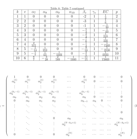
⎤ ⎥ ⎥ ⎥ ⎥ ⎥ ⎥ ⎥ ⎦ (22) The order and the error constant of the SDGBDF (17) are shown in tables 7 and 8 fork= 1(1)10.

For the numerical solution of (1) the second deriva-tive BVMs with (k₁, k₂)-boundary conditions, the main method

k2

i=−k1

αi+k1yn+i=h k2

i=−k1

βi+k1fn+i+h2 k2

i=−k1

λi+k1fn+i ,

(23)

n=k₁, . . . , N−k₂

y₀, . . . , yk1−1, yN, . . . , yN+k2−1 f ixed

together withk₁−1 additional initial methods

k

i=0

α(_ij)y_i=h

k

i=0

β_i(j)f_i+h2

k

i=0

λ(_ij)f_i , (24)

j= 1, . . . , k₁−1 andk₂ ﬁnal methods

k

i=0α(kj−)iyN−i=h

k

i=0βk(j−)ifN−i

+h2k_i₌₀λ(_kj₋)_if_N ₋_i , j=N, . . . , N+k₂−1 (25) can be expressed as

A_Ny−hB_Nf−h2C_Nf=

⎛ ⎜ ⎜ ⎜ ⎜ ⎜ ⎜ ⎜ ⎜ ⎜ ⎜ ⎜ ⎜ ⎜ ⎜ ⎜ ⎜ ⎜ ⎜ ⎝

_k₁₋₁

i=0 (αiyn+i−hβifn+i−h2λifn+i)

.. .

α₀yn+k1−1−hβ0fn+k1−1−h2λ0fn+k1−1

0 .. . 0

αkyn+N −hβkfn+N −h2λkfn+N

.. .

_k₂

i=1(αk1+iyn+N−1+i−hβk1+i×

fn+N−1+i−h2λk1+ifn+N−1+i)

⎞ ⎟ ⎟ ⎟ ⎟ ⎟ ⎟ ⎟ ⎟ ⎟ ⎟ ⎟ ⎟ ⎟ ⎟ ⎟ ⎟ ⎟ ⎟ ⎠ (26)

whereAN andBN are deﬁned similarly as in (12), while

CN is given in (41), y = (y0, . . . , yN)T is the discrete

solution,fand f are the ﬁrst and second derivatives re-spectively, h is the step size and AN, BN and CN are

(N + 1)×(N + 1) matrices with the same structure as those in (12).

To analyze the stability of a speciﬁc method (26), (see, [30]) we apply (23) on the test problem

y =λy, y=λ2y (27)

to determine its boundary locus. The class of methods (17) yields the characteristics equation:

k

j=0

αjzj−(qβv+q2)zv= 0, q=λh, q∈C (28)

wherev is deﬁned as in (16). Letting z =eiθ _{we obtain}

two roots (since (28) is quadratic inq) for corresponding values ofk andv to give the stability regions deﬁned by

q given in Figures 1 and 2 for odd and even values of

krespectively. Compared with the generalization of the BDF by Brugnano and Trigiante [8] discussed in section 1 the proposed class of methods (17) are found to have higher orderp=k+ 1 and a smaller error constant for corresponding values of the steplengthk, although with need to compute the second derivative for which it is not expensive for some autonomous stiﬀ systems.

5

Implementation Procedure

In this section the implementation procedure for the SDGBDF(17) of order 4 and 5 as BVMs in the sense of Brugnano and Trigiante [7, 8] is presented. The pro-posed class of methods (17) is used with the following additional initial methods:

k

j=0

α∗_jy_j =hβ_if_i+h2f_i, i= 1,2,· · ·, v−1 (29)

and ﬁnal methods:

k

j=0

α∗_jyj=hβifi+h2fi, i=v+ 1,· · ·, N (30)

The SDGBDF (17) of order 4 which isA₂,1-stable and

0₂,1-stable with (2,1)-boundary conditions requires two

initial methods (y₀is already provided by the initial value deﬁning the ODE (1)) and one ﬁnal method. The fourth order SDGBDF (17) is given as:

−1

6yn+2yn+1− 5 2yn+2+

2

3yn+3=−hfn+2+h

2_f

n+2 (31)

The main method ( 31) can be written in the form

−1

6yn−2+ 2yn−1− 5 2yn+

2

3yn+1=−hfn+h

2_f

n (32)

n= 2,· · ·, N−1

IAENG International Journal of Applied Mathematics, 48:1, IJAM_48_1_01

(5)

and used with the following initial method

2 3y0−

5

2y1+ 2y2− 1

6y3=hf1+h

2_f

1 (33)

and ﬁnal method

2 9yN−3−

3

2yN−2+6yN−1− 85

18yN =− 11

3 hfN+h

2_f

N (34)

Similarly the SDGBDF (17) of order 5

₁

18yn−1₂yn+1+ 3yn+2−55₁₈yn+3+1₂yn+4

=−5₃hfn+3+h2fn+3

(35)

n= 3,· · ·, N−1

with the initial methods

1 2y0−

55

18y1+ 3y2− 1 2y3+

1 18y4=

5

3hf1+h

2_f 1 (36)

and

−1 12y0+

4 3y1−

5 2y2+

4 3y3−

1

12y4= 2h

2_f

2 (37)

and the ﬁnal method

−1

8yN−4+8₉yN−3−3yN−2+ 8yN−1−415₇₂yN

=−25₆hfN +h2fN

(38)

will be taken together as a BVM.

The methods (31 and 35) are implemented as BVMs ef-ficiently by composing the main methods and the addi-tional methods as simultaneous numerical integrators for the IVP(1). In particular for linear problems, we can solve (1) directly from the start with Gaussian elimina-tion partially using pivoting and for nonlinear problems we can use a modified Newton-Raphson method. In each case, the main methods and the additional methods are combined as BVMs to give a single matrix of finite dif-ference equations which simultaneously provides the val-ues of the solution and the first derivatives generated by the sequences {yn},{yn}, n = 0, . . . , N, where the

sin-gle block matrix equation is solved while adjusting for boundary conditions ([35]).

6

Numerical

Experiments

with

SDGBDF

We consider the following stiﬀ problems (linear and non-linear) to illustrate the implementation and examine the accuracy of the SDGBDF (17) of orders p=4 (31) and 5 (35) implemented as block methods. The fourth order method (17) and the ﬁfth order method (17) are denoted by SDGBDF4 and SDGBDF5 respectively.

Problem 1: A linear stiﬀ problem, see [4, 10, 25, 43]

y₁ =−21y₁+ 19y₂−20y₃, y₁(0) = 1,

y₂= 19y₁−21y₂+ 20y₃, y₂(0) = 0,

y₃ = 40y₁−40y₂+ 40y₃, y₃(0) =−1.

The SDGBDF4 is applied to this problem and the maximum absolute errors (|y(x) − yn|) in the

inter-val 0 < x < 10 are compared with the Adams type block method of Akinfenwa [4] (ATBM7), the general-ized backward diﬀerentiation formula of Brugnano and Trigiante [10](GBDF8) and theL(α)-stable block multi-step method of Ehigie and Okunuga [25] denoted by EH-OK5. The rate of convergence, Rateh = log2(errerr2hh) whereerr_his the maximum absolute error at steplength

h= ₂n_.1₁₀₀, n= 0,1,2,3 and 4 , is used to verify the order of the methods. Also in comparison with the CBDF₅

of degree s = 5 in Ramos and Garcia-Rubio [43], the AbsErr(t_f) is obtained by the SDGBDF4 in the inter-val 0≤x≤1. It is observed that the new method even though it is of order 4 performs better than the EH-OK5, the ATBM7 and the GBDF8 of orders 5, 7 and 8 respec-tively. The details of the numerical results are displayed in Table 1. In Table 2, it is noticed that the SDGBDF4 is comparable with the EH-OK5 in [25] and theCBDF₅

[image:5.595.38.292.106.410.2]

in [43].

Table 1: Maximum absolute error, M ax₁<i<N|yi(x)−

yi,n|for problem 1,h= ₂n_.1₁₀₀

n SDGBDF4 EH-OK5 GBDF8 ATBM7 (Rate) (Rate) (Rate) (Rate) 0 2.28×10−17 3.21×10−13 1.19×10−3 3.95×10−6 1 1.56×10−18 1.01×10−14 1.39×10−5 2.91×10−8

(3.87) (4.99) (6.42) (7.08) 2 1.02×10−19 3.18×10−16 1.08×10−7 2.21×10−10

(3.93) (4.99) (7.00) (7.06) 3 6.21×10−21 9.96×10−18 1.08×10−9 6.65×10−13

(4.04) (5.00) (6.64) (8.36) 4 9.45×10−23 3.11×10−19 9.41×10−12 2.69×10−15

(6.04) (5.00) (6.84) (7.95)

Table 2: Numerical results in comparison with CBDF₅

and EH-OK5 for problem 1 the interval 0≤x≤1

Steps SDGBDF4 EH-OK5 CBDF5

(Rate) (Rate) (Rate) 20 1.12×10−11 3.04×10−11 4.12×10−12 40 7.01×10−13 9.75×10−13 1.33×10−12

(4.00) (4.96) (4.95) 80 4.47×10−14 2.25×10−14 4.31×10−15

(3.97) (5.43) (4.95) 160 1.47×10−15 9.69×10−16 2.55×10−15

(4.93) (4.53) (0.75)

Problem 2: Non-linear stiﬀ system solved by Wu and Xia [44]

y₁ =−1002y₁+ 1000y₂2, y₁(0) = 1,

y₂=y₁−y₂(1 +y₂), y₂(0) = 1,

IAENG International Journal of Applied Mathematics, 48:1, IJAM_48_1_01

(6)

The exact solution of the system is given by

y₁(x) =e−2x, y₂(x) =e−x

Problem 2 is solved using SDGBDF5 with a steplength

h= 0.008 in the range 0≤x≤1. The maximum error (Max|y_i−y(x_i)|) of the method is given in Table 3. From Table 3, it is obvious that the new method of order 5 is better than the methods of Ehigie et al [24] and Wu-Xia [44] and very comparable with the method of Jator and Sahi [36] which are of orders 5, 6 and 8 respectively.

Problem 3: Singularly Perturbed Problem

Table 3: Maximum error, Max|yi−y(xi)|, for problem 2

Method N h y1 y2

(Max|y_i−y(x_i)|) (Max|y_i−y(x_i)|) SDGBDF5 125 0.008 1.80_×10−15 6.11_×10−16 Ehigie et al 125 0.008 3.88×10−14 3.10×10−14

(BVM3)

Jator-Sahi 125 0.008 1.63×10−14 0.00 Wu-Xia 500 0.002 2.56×10−07 8.02×10−08

y₁ =−(2 + 104)y₁+ 104y2₂, y₂ =y₁−y₂−y₂2,

y₁(0) = 1, y₂(0) = 1 The exact solution is y₁ = e−2t_{, y}

2 = e−t, see [30].

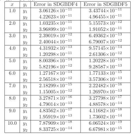
[image:6.595.304.533.266.402.2]

The SDGBDF4 and the SDGBDF5 are applied to Prob-lem 3 and the results are compared with the theoreti-cal solution. The SDGBDF5 performs better than the SDGBDF4 as expected, see Table 4. Furthermore, take note that the graphs of the exact and the numerical so-lutions in Figures 3 and 4 coincide.

Table 4: Absolute error in problem 3, h = 0.01, Error

yi=|yi−y(xi)|, i= 1,2

x y_i Error in SDGBDF4 Error in SDGBDF5 1.0 y1 3.06126×10−11 3.43744×10−11

y2 4.22623×10−11 4.96455×10−11 2.0 y₁ 1.03235×10−11 5.15573×10−12

y₂ 3.96899×10−11 1.91052×10−11 3.0 y₁ 2.39019×10−12 6.49362×10−13

y₂ 2.40044×10−11 6.79007×10−12 4.0 y₁ 4.31932×10−13 9.57145×10−14

y₂ 1.20298×10−11 2.61306×10−12 5.0 y₁ 8.00396×10−14 1.20228×10−14

y₂ 5.82196×10−12 9.28587×10−13 6.0 y₁ 1.27167×10−14 1.77133×10−15

y₂ 2.56518×10−12 3.57306×10−13 7.0 y₁ 2.18299×10−15 2.22482×10−16

y₂ 1.15005×10−12 1.26970×10−13 8.0 y₁ 3.27871×10−16 3.27798×10−17

y2 4.79014×10−13 4.88578×10−14 9.0 y₁ 4.83562×10−17 4.11682×10−18

y₂ 1.95919×10−13 1.73602×10−14 10.0 y1 7.87909×10−18 6.06524×10−19

y2 8.33725×10−14 6.67981×10−15

Problem 4: Van der Pol equations, see [30] (nonlinear problem)

y₁=y₂, y₂ =−y₁+ 10y₂(1−y₁2),

y₁(0) = 2, y₂(0) = 0.

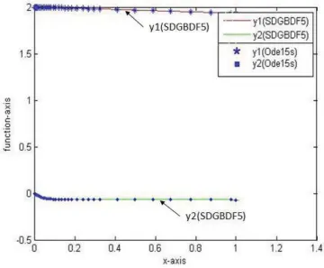
For problem 4, it is clearly seen from Table 5 and Figures 5 and 6 that the proposed class of methods compares favorably with the solution from the Ode15s in MATLAB.

Problem 5: Robertson’s equation, see [30] (nonlinear

Table 5: Errors in problem 4 using the modulus of the solution of SDGBDF minus the solution of Ode15s,h= 0.001. Error y_i=|y_iSDGBDF −y_iOde₁₅_s|,i= 1,2

x y_i Error in SDGBDF4 Error in SDGBDF5 1.0 y₁ 1.32308×10−4 1.82747×10−5

y2 8.31878×10−6 1.09583×10−6 5.0 y₁ 3.36208×10−4 1.47667×10−4

y₂ 2.22430×10−5 3.98291×10−6 10.0 y1 3.67025×10−5 2.25767×10−4

y2 1.98333×10−6 1.32565×10−5 15.0 y₁ 2.46188×10−5 6.92917×10−4

y₂ 3.09782×10−5 7.75023×10−5 20.0 y1 9.04906×10−5 2.00872×10−4

y2 1.10280×10−5 6.98618×10−6

problem)

y₁=−0.04y₁+104y₂y₃, y₂= 0.04y₁−104y₂y₃−3×107y₂2,

y₃ = 3×107y2₂, y₁(0) = 1, y₂(0) = 0, y₃(0) = 0.

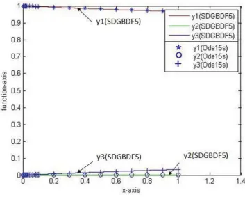
Problem 5 is solved by the SDGBDF4 and the SDGBDF5 and the results are compared with the solution from the Ode15s in MATLAB. It is observed from Table 6 and Fig-ures 7 and 8 that the new methods are very comparable with the Ode15s in MATLAB.

Table 6: Errors in problem 5 using the modulus of the solution of SDGBDF minus the solution of Ode15s,h= 0.0001. Erroryi =|yiSDGBDF−yiOde15s|, i= 1,2,3

x y_i Error in SDGBDF4 Error in SDGBDF5 1.0 y1 2.31233×10−5 6.11248×10−6

y2 3.68698×10−9 9.74789×10−10

y3 2.31270×10−5 6.11346×10−6 3.0 y₁ 3.91192×10−6 3.91187×10−6

y₂ 4.93245×10−10 4.93239×10−10

y₃ 3.91241×10−6 3.91236×10−6 5.0 y₁ 1.02179×10−6 1.02175×10−6

y₂ 2.95023×10−10 2.95027×10−10

y₃ 1.02149×10−6 1.02146×10−6 7.0 y₁ 4.48772×10−5 4.48771×10−5

y₂ 4.22263×10−9 4.22262×10−9

y₃ 4.48814×10−5 4.48814×10−5 10.0 y₁ 7.35061×10−5 7.35060×10−5

y₂ 5.76555×10−9 5.76555×10−9

y₃ 7.35118×10−5 7.35118×10−5

IAENG International Journal of Applied Mathematics, 48:1, IJAM_48_1_01

[image:6.595.44.277.541.773.2]

(7)

[image:7.595.57.533.311.795.2]

Table 7: The Coeﬃcients, Error Constant (EC) and Orderpof SDGBDF(18) fork= 1(1)10

k

v

α

₀

α

₁

α

₂

α

₃

α

₄

α

₅

α

₆

1

2

-2

0

2

−

1₂

4

−

7₂

0

3

2

−

1₆

2

−

5₂ 2₃

0

4

3

₁₈1

−

1₂

3

−

55₁₈ 1₂

0

5

3

₄₅1

−

1₄

2

−

49₁₈

1

−

₂₀1

0

6

4

−

₁₂₀1 ₄₅4

−

1₂ 8₃

−

217₇₂ 4₅

−

₃₀1

7

4

−

₂₈₀1 ₄₅2

−

₁₀3

2

−

205₇₂ 6₅

−

₁₀1

8

5

₇₀₀1

−

₅₆1 1₉

−

1₂ 5₂

−

5449₁₈₀₀

1

9

5

₁₅₇₅1

−

₁₁₂1 ₆₃4

−

1₃

2

−

5269₁₈₀₀ 4₃

10

6

−

₃₇₈₀1 ₅₂₅2

−

₁₁₂3 ₆₃8

−

1₂ 12₅

−

5489₁₈₀₀

Table 8: Table 7 continued

k

v

α

₇

α

₈

α

₉

α

₁₀

β

_v

γ

_v

EC

p

1

0

-2

1

1₃

2

0

-3

1

1₆

3

2

0

-1

1

−

₃₀1

4

3

0

−

5₃

1

−

₆₀1

5

3

0

−

2₃

1

₂₁₀1

6

4

0

−

7₆

1

₄₂₀1

7

4

₃₁₅2

0

−

1₂

1

−

₁₂₆₀1

8

5

−

₁₄1 ₂₅₂1

0

−

₁₀9

1

−

₂₅₂₀1

9

5

−

1₇ ₆₃1

−

₁₀₀₈1

0

−

2₅

1

₆₉₃₀1

10

6

8₇

−

₂₈3 ₁₈₉2

−

₁₆₈₀1

−

11₁₅

1

₁₃₈₆₀1

11

A

_N

=

⎛

⎜

⎝

1

0

· · ·

0

· · · ·

0

α

(1)₀

α

(1)₁

α

₂(1)

α

(1)₃

· · ·

α

(1)_k

0

· · · ·

0

..

.

..

.

..

.

..

.

· · ·

..

.

..

.

· · · ·

..

.

α

₀(k1−1)

α

₁(k1−1)

α

(₂k1−1)

α

(₃k1−1)

· · ·

α

_k(k1−1)

..

.

· · · ·

..

.

α

₀

α

₁

α

₂

α

₃

· · ·

α

_k

0

· · · ·

0

α

₀

α

₁

α

₂

· · ·

α

_k₋₁

α

_k

0

· · ·

0

..

.

. ..

. .. ... ...

..

.

..

.

. ..

. .. ... ...

0

..

.

. ..

0

α

₀

· · ·

· · · ·

α

_k

..

.

. ..

..

.

α

(N−k2+1)

0

· · ·

· · · ·

α

(kN−k2+1)

..

.

. ..

..

.

..

.

· · ·

· · · ·

..

.

0

· · ·

0

α

₀(N)

· · ·

· · · ·

α

(_kN)

⎞

⎟

⎠

(39)

IAENG International Journal of Applied Mathematics, 48:1, IJAM_48_1_01

(8)

B

_N

=

⎛

⎜

⎝

0

· · ·

0

· · · ·

0

β

₀(1)

β

₁(1)

β

₂(1)

β

₃(1)

· · ·

β

_k(1)

0

· · · ·

0

..

.

..

.

..

.

..

.

· · ·

..

.

..

.

· · · ·

..

.

β

₀(k1−1)

β

₁(k1−1)

β

₂(k1−1)

β

₃(k1−1)

· · ·

β

_k(k1−1)

..

.

· · · ·

..

.

β

₀

β

₁

β

₂

β

₃

· · ·

β

_k

0

· · · ·

0

β

₀

β

₁

β

₂

· · ·

β

_k₋₁

β

_k

0

· · ·

0

..

.

. ..

. .. ... ...

..

.

..

.

. ..

. .. ... ...

0

..

.

. ..

0

β

₀

· · ·

· · · ·

β

_k

..

.

. ..

..

.

β

(N−k2+1)

0

· · ·

· · · ·

β

(kN−k2+1)

..

.

. ..

..

.

..

.

· · ·

· · · ·

..

.

0

· · ·

0

β

₀(N)

· · ·

· · · ·

β

_k(N)

⎞

⎟

⎠

(40)

C

_N

=

⎛

⎜

⎝

0

· · ·

0

· · · ·

0

λ

(1)₀

λ

(1)₁

λ

(1)₂

λ

(1)₃

· · ·

λ

(1)_k

0

· · · ·

0

..

.

..

.

..

.

..

.

· · ·

..

.

..

.

· · · ·

..

.

λ

₀(k1−1)

λ

₁(k1−1)

λ

(₂k1−1)

λ

(₃k1−1)

· · ·

λ

_k(k1−1)

..

.

· · · ·

..

.

λ

₀

λ

₁

λ

₂

λ

₃

· · ·

λ

_k

0

· · · ·

0

λ

₀

λ

₁

λ

₂

· · ·

λ

_k₋₁

λ

_k

0

· · ·

0

..

.

. ..

. .. ... ...

..

.

..

.

. ..

. .. ... ...

0

..

.

. ..

0

λ

₀

· · ·

· · · ·

β

_k

..

.

. ..

..

.

λ

₀(N)

· · ·

· · · ·

λ

(_kN)

..

.

. ..

..

.

..

.

· · ·

· · · ·

..

.

0

· · ·

0

λ

₀(N+k2−1)

· · ·

· · · ·

λ

(_kN+k2−1)

⎞

⎟

⎠

(41)

(9)

Figure 1: Stability region (exterior of closed curves) of (17), k=1 (2) 31

(10)

Figure 2: Stability region (exterior of closed curves) of (17), k=2 (2) 32

(11)

[image:11.595.114.461.113.398.2]

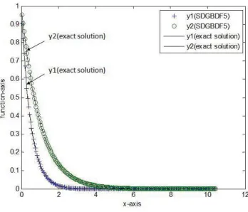
Figure 3: Numerical Results for Problem 3 with SDGBDF4, h=0.01

IAENG International Journal of Applied Mathematics, 48:1, IJAM_48_1_01

[image:11.595.110.459.455.753.2]

(12)

[image:12.595.128.442.108.407.2]

[image:12.595.102.463.456.753.2]

(13)

[image:13.595.107.461.115.410.2]

[image:13.595.107.461.464.747.2]

(14)

7

Conclusion

The second derivative generalized backward diﬀerentia-tion formulae (SDGBDF) have been introduced in secdiﬀerentia-tion (4). This class of methods is Av,k−v-stable and 0v,k−v

-stable with (v, k-v)-boundary conditions for values of

k ≥ 1 with order p = k+ 1. The new class of meth-ods is found to be suitable for the solution of stiﬀ IVPs in ODEs for reason of their stability. The class of meth-ods (17) also ﬁnds application in the solution of boundary value problems, see [35, 39].

Acknowledgement

The authors are grateful to Prof. M.N.O. Ikhile (Director of ARLAB) and the anonymous reviewers for comments that have improved the quality of this work.

References

[1] L. Aceto, P. Ghelardoni and C. Magherini, Boundary Value Methods as an extension of Numerovs method for Sturm-Liouville eigenvalue estimates, Appl. Nu-mer. Math., 59, (2009), 1644-1656.

[2] L. Aceto and C. Magherini, On the relations between B2VMs and Runge-kutta collocation methods, Jour-nal of ComputatioJour-nal and Applied Mathematics, 231, (2009), 11-23.

[3] L. Aceto, P. Ghelardoni and C. Magherini, PGSCM: A family of P-stable Boundary Value Methods for second-order initial value problems,Journal of Com-putational and Applied Mathematics, 236, (2012), 3857-3868.

[4] O. A. Akinfenwa, Seven step Adams Type Block Method with Continuous Coeﬃcient for Periodic Or-dinary Diﬀerential Equation,Word Academy of Sci-ence, Engineering and Technology, 74, (2011), 848-853 .

[5] B. I. Akinnukawe, O. A. Akinfenwa and S. A. Okunuga, L-Stable Block Backward Diﬀerentiation Formula for Parabolic Partial Diﬀerential Equations,

Ain Shams Engineering Journal, 7, (2016), 867-872.

[6] L. Brugnano and D. Trigiante, Convergence and sta-bility of boundary value methods for ordinary diﬀer-ential equations,Journal of Computational and Ap-plied Mathematics, 66, (1996), 97-109.

[7] L. Brugnano, Boundary Value Methods for the Numerical Approximation of Ordinary Diﬀerential Equations, Lecture Notes in Comput. Sci., 1196, (1997), 78-89.

[8] L. Brugnano and D. Trigiante, Solving Diﬀerential Problems by Multistep Initial and Boundary Value Methods, Gordon and Breach Science Publishers, Amsterdam, 1998a.

[9] L. Brugnano and D. Trigiante, Boundary Value Methods: the third way between linear multistep and Runge-Kutta methods, Comput. Math. Appl., 36, (10-12), (1998b), 269-284.

[10] L. Brugnano and D. Trigiante, Block Implicit meth-ods for ODEs in: D. Trigiante (Ed.), Recent trends in Numerical Analysis, New York: Nova Science Publ. inc, 2001.

[11] L. Brugnano and C. Magherini, Blended Implicit Methods for solving ODE and DAE problems and their extension for second order problems, Jour. Comput. Appl. Mathematics, 205, (2007), 777-790.

[12] L. Brugnano, F. Iavernaro and T. Susca, Hamilto-nian BVMs (HBVMs): implementation details and applications, AIP Conf. Proc., 1168, (2009), 723-726.

[13] L. Brugnano, F. Iavernaro and D. Trigiante, Hamil-tonian BVMs (HBVMs): a family of drift-free meth-ods for integrating polynomial Hamiltonian systems,

AIP Conf. Proc., 1168, (2009), 715-718.

[14] L. Brugnano, F. Iavernaro and D. Trigiante, Hamil-tonian boundary value methods (Energy preserving discrete line integral methods), Journal of Numeri-cal Analysis, Industrial and Applied Mathematics, 5, 1-2, (2010), 17-37.

[15] L. Brugnano, F. Iavernaro and D. Trigiante, A note on the eﬃcient implementation of Hamiltonian BVMs.Journal of computational and Applied Math-ematics, 236, (2011), 375-383.

[16] L. Brugnano, G. Frasca Caccia and F. Iavernaro, Eﬃcient implementation of Gauss collocation and Hamiltonian Boundary Value Methods. Numer. Al-gor., 65, (2014), 633-650.

[17] L. Brugnano, F. Iavernaro and D. Trigiante, Anal-isys of Hamiltonian Boundary Value Methods (HB-VMs): a class of energy preserving Runge-Kutta methods for the numerical solution of polynomial Hamiltonian systems, Communications in Nonlin-ear Science and Numerical Simulation, 20, 3, (2015), 650-667.

[18] R. L. Burden and J. D. Faires, Numerical Analy-sis (9th Edition), Brooks/Cole, Cengage Learning, Boston, 2011.

[19] J. R. Cash, On integration of stiff systems of ordi-nary differential equations using extended backward differentiation formula, Numer. Math., 3, (1980), 235-246.

[20] J. R. Cash, Second Derivative Extended Backward Diﬀerentiation Formulas for the Numerical Integra-tion of Stiﬀ Systems, SIAM Journal of Numerical Analysis, 18(1), (1981), 21-36.

IAENG International Journal of Applied Mathematics, 48:1, IJAM_48_1_01

(15)

[21] J. R. Cash, The Integration of Stiff initial value problems in ODEs using modified extended back-ward differentiation formula, Comput. Math. Appl., 9, (1983), 645-657.

[22] C. F. Curtis and J. O. Hirschfelder, Integration of Stiﬀ Equations, National Academy of Sciences, 38, (1952), 235-243.

[23] G. Dahlquist, A special stability problem for linear multistep methods,BIT, 3, (1963), 27-43.

[24] J.O. Ehigie, S.N. Jator, A.B. Sofoluwe and S.A. Okunuga, Boundary value technique for initial value problems with continuous second derivative multi-step method of Enright,Computational and Applied Mathematics, 33(1), (2014), 81-93.

[25] J.O. Ehigie and S.A. Okunuga, L(α)-stable second derivative block multistep formula for stiﬀ initial value problems,IAENG International journal of Ap-plied Mathematics, 44(3), (2014), 157-162.

[26] A. K. Ezzeddine and G. Hojjati, Hybrid Extended Backward Diﬀerentiation Formulas for Stiﬀ Systems,

International Journal of Nonlinear Science, 12(2), (2011), 196-204.

[27] S. O. Fatunla, Block methods for second order IVPs,

Intern. J. Compt. Maths., 41, (1991), 55-63.

[28] V. G. Ganzha and E. V. Vorozhtsov, Computer-Aided Analysis of Diﬀerence Schemes for Partial Diﬀerential Equations, John Wiley and Sons., Inc., Canada, 1996.

[29] C. W. Gear, Numerical initial value problems in ordinary diﬀerential equations, Prentice-Hall, New Jersey, (1971), 253pp.

[30] E. Hairer and G. Wanner,Solving Ordinary Differ-ential Equations II: Stiff and DifferDiffer-ential Algebraic Problems, Second Revised Edition, Springer Verlag, Germany, 1996.

[31] P. Henrici, Discrete Variable Methods in Ordinary Diﬀerential Equations, Wiley, New York, 1962.

[32] F. Iavernaro and F. Mazzia, Block-Boundary Value Methods for the solution of Ordinary Diﬀerential Equations, SIAM J. Sci. Comput., 21(1), (1999), 323-339.

[33] F. Iavernaro and B. Pace, Conservative Block-Boundary Value Methods for the Solution of Polyno-mial Hamiltonian Systems, AIP Conf. Proc., 1048, (2008), 888-891.

[34] Z. B. Ibrahim, K. I. Othman and M. Suleiman, Vari-able Step Block Backward Diﬀerentiation Formula for Solving First Order Stiﬀ Odes, World Congress on Engineering, (2007), 785-789.

[35] S. N. Jator and J. Li, Boundary Value Methods via a Multistep Method with Variable Coeﬃcients for Second order initial and boundary value problems,

International Journal of Pure and Applied Mathe-matics, 50(3), (2009), 403-420.

[36] S. N. Jator and R.K. Sahi, Boundary value tech-nique for initial value problems based on Adams-type second derivative methods,International Jour-nal of Mathematical Education in Science and Tech-nology, 41(6), (2010), 819-826.

[37] J. D. Lambert,Numerical methods for ordinary dif-ferential equations, John Wiley and Sons, New York, 1991.

[38] J. R. LeVeque, Finite Diﬀerence Methods for Or-dinary and Partial Diﬀerential Equations, SIAM, 2007.

[39] Z.A. Majid, M.M. Hasni and N. Senu, Solving Sec-ond Order Linear Dirichlet and Neumann Bound-ary Value Problems by Block Method, IAENG In-ternational Journal of Applied Mathematics, 43(2), (2013), 71-76.

[40] F. Mazzia, Boundary Value Methods for the nu-merical solution of Boundary Value Problems in Diﬀerential-Algebraic Equations, Bollettino dellU-nione Matematica Italiana, (7) 11-A, (1997), 579-593.

[41] F. Mazzia and I. Sgura, Numerical approximation of nonlinear BVPs by means of BVMs, Appl. Numer. Math., 42 (2002), 337-352.

[42] H. Musa, A 2-Point Variable Step Size Block Ex-tended Backward Diﬀerentiation Formula for Solv-ing Stiﬀ IVPs,Nigerian Association of Mathematical Physics, 28(2), (2014), 93-100.

[43] H. Ramos and R. Garcia-Rubio, Analysis of a Chebyshev-based Backward Diﬀerentiation Formu-lae and Relation with Runge-kutta Collocation Methods,International Journal of Computer Math-ematics, 88, 3, (2011), 555-577.

[44] X. Wu and J. Xia, Two low accuracy methods for stiﬀ systems,Appl. Math. Comput., 123, (2001), 141-153.