A Bayesian approach to comparing theoretic models to observational data: A case study from solar flare physics

(1)

arXiv:1102.0242v1 [astro-ph.SR] 1 Feb 2011

S. Adamakis1 C. L. Raftery2

R. W. Walsh1

P. T. Gallagher2

ABSTRACT

Solar flares are large-scale releases of energy in the solar atmosphere, which are characterized by rapid changes in the hydrodynamic properties of plasma from the pho-tosphere to the corona. Solar physicists have typically attempted to understand these complex events using a combination of theoretical models and observational data. From a statistical perspective, there are many challenges associated with making accurate and statistically significant comparisons between theory and observations, due primarily to the large number of free parameters associated with physical models. This class of ill-posed statistical problem is ideally suited to Baysian methods. In this paper, the solar flare studied by Raftery et al. (2009) is reanalysed using a Baysian framework. This enables us to study the evolution of the flare’s temperature, emission measure and energy loss in a statistically self-consistent manner. The Baysian-based techniques confirm that both conductive and non-thermal beam heating play important roles in heating the flare plasma during the impulsive phase of this event.

Subject headings: Sun: corona — Sun: flares — methods: statistical

1. Introduction

Solar flares are triggered by the instability of the magnetic field. This can result in the direct or indirect heating of chromospheric plasma leading to the process known as “chromospheric evaporation” (Milligan et al. 2006a,b). There are two ways to provoke evaporation (chromospheric

1_{Jeremiah Horrocks Institute for Astrophysics and Supercomputing, University of Central Lancashire, Preston,}

PR1 2HE, UK

(2)

plasma upflow): using thermal energy and/or using non-thermal energy according to the energy release mechanisms (Mariska et al. 1993). In the thermal energy model, heat is unleashed in the coronal portion of the loop (possibly because of magnetic reconnection). Then the thermal energy is carried downward to the upper chromosphere via conduction, where the deposited energy heats the plasma and stimulates it to move slowly upward. In the non-thermal energy model, the energy release (again in the corona) is in the form of a non- thermal electron beam. Electrons then collide with dense chromospheric plasma, which they heat, causing the plasma to expand both upward at very high speeds and downward at lower speeds.

This paper will focus on the statistical analysis of the observations outlined in Raftery et al. (2009) and will be compared with results from the Enthalpy Based Thermal Evolution of Loops (EBTEL) model (Klimchuk et al. 2008). Comparing to Raftery et al. (2009) this research will han-dle the statistics with care to derive which of the thermal or non-thermal heat flux is more dominant, during a single flare event, using model comparison techniques (Kass 1993; Kass & Greenhouse 1989; Kass & Raftery 1995; Raftery 1996; Clyde et al. 2007; Adamakis et al. 2008). Furthermore, the method used here treats the uncertainties for the time constraints with equal respect as the uncertainties of the temperature and emission measure, which are difficult to incorporate into our analysis regarding Classical statistics. The thermal heat flux is proportional to the non-thermal heat flux plus a constant background heat flux. The parameter space is extended with the addition of the radius of the loop in order to make the model more realistic. Last but not least, the ratios between the radiative loss rate of the transition and the corona, the average coronal and apex temperature, and the coronal base and apex temperature are assumed to be free parameters so that their values will be decided by the data. For more information about these parameters refer to Section 3.

(3)

2. Previous Work

2.1. Observations of a C-Class Solar Flare

The temporal evolution of temperature and emission measure in a C3.0 solar flare observed on March 26, 2002 has been analysed. During a typical solar flare, the temperature rises from less than one MK up to _∼ 20 MK, and then cools down to the pre-flare temperatures. In the example under consideration here, Raftery et al. (2009) used different instruments to track this evolution: the Reuven Ramaty High Energy Solar Spectroscopic Imager (RHESSI; > 5 MK), GOES-12 (5₋30 MK), the Transition Region and Coronal Explorer (TRACE 171 ˚A ; 1 MK), and the Coronal Diagnostic Spectrometer (CDS;_∼0.03₋8 MK). We note here that TRACE data were not included in the emission measure analysis. This is as a result of the instrument being sensitive to multiple emission lines, making it complex to define the contribution function. The reader is referred to Raftery et al. (2009) which outlines the reasons why and at which particular time of the flare each particular instrument was employed.

The flare began with evidence of pre-flare heating at its onset. This was followed by explosive chromospheric evaporation during the impulsive phase and gentle chromospheric evaporation during the early decay phase. It is believed that the plasma reached a peak temperature of just more than 13 MK in approximately 10 min. Conduction losses dominated over radiative losses for the initial_∼ 300 s of the post-flare decay, whereas for the next_∼4000 s, radiative losses prevailed. Raftery et al. (2009) concluded that approximately equal direct and non-thermal heating mechanisms produced the data observed according only to an estimation of the ratio between the thermal and non-thermal heating rate, which is of course very critical. The best fit and parameter intervals were derived using an acceptable fit to the data by eye.

2.2. The EBTEL Model

(4)

To reflect the physical processes taking place within the standard flare model, the EBTEL model allows for both thermal and non-thermal heating of the plasma in the system. It has been noted that proton precipitation is not included (see Aschwanden 2005). Proton beams are expected to excite strong kinetic Alfv´en waves. The turbulence caused by kinetic Alfv´en waves contains enough energy to produce the non-thermal velocities observed in flares, and therefore could contribute to impulsive primary plasma heating between the reconnection regions and the flare footpoints.

Deviations of the observations from the model could be caused by two distinct reasons: First, the EBTEL model treats the effects of the non-thermal electron beam in a very simple way. It is assumed that all the beam’s energy goes into evaporating plasma upwards into the loop, which is reasonable for gentle evaporation. However, for explosive evaporation, some of the beam energy will be used to drive chromospheric downflows, making the total observed non-thermal energy larger than that predicted by the EBTEL model. Second, the flare loop is almost certainly constructed of many strands that are heated at different times. Raftery et al. (2009) assume the flaring loop consists of individual strands, all heated simultaneously. Therefore they model the loop as one “fat strand”. However, some strands are likely to be heated at a different time compared to this solid structure.

3. Defining the Model Parameters

3.1. Data Distribution

The errors in temperature come from the width of the contribution function for the particular emission line (for the CDS points) and from the width of the instrument response function for GOES and TRACE. The RHESSI temperature error comes from the uncertainty in the fit to the Maxwell Boltzmann distribution.

As there is no information about the form of the errors, it is assumed that the errors between the observed temperatures and emission measures and those predicted from the model are normally distributed with mean zero and standard deviation derived from the error bars (we assume “3σ” belief; see Adamakis et al. 2008). This means that the likelihood will be of the form:

p(D_|P) = 1

(2π)(n1+n2)/2(Q_in1₌₁σi1) (Qn2i=1σi2)

exp   − n1 X i=1

Ti−Tbi(P)

2

2σ2

i1 − n2 X i=1

EMi−EMdi(P)

2

2σ2

i2

  

I maxT <3_×107,

(5)

respec-tively proposed by the EBTEL model, P is the parameter space (see end of Section 3), n1 is the

number of observed temperature values, n2 is the number of observed emission measure values, σi1 are the standard deviations of the temperature errors, σi2 are the standard deviations of the

emission measure errors and _I(_·) is the indicator function which is given by:

I maxT <3_×107=

(

1, if maxT <3_×107K 0, otherwise.

where maxT is the maximum temperature value of the cooling curve. The temperature profile is restricted to not exceed 30 MK because it is believed that temperatures above this threshold will create unphysical data.

3.2. Parameters for Non-Thermal Heat Flux

As discussed in Section 1, one of our aims is to compare which of the Half Gaussian and Full Gaussian functions for the non-thermal heat flux fits better to the data observed. In the case of the Half Gaussian the non-thermal heat flux function is given by the form:

F(t) =

(

A √

2πσ1exp

h

−(t₂−_σµ2)2 1

i

, t_≤µ

0, t > µ

wheretis the time, µis the time that maximise the non-thermal heat flux function (which can be adopted as a parameter), σ1 is a value that defines the width of this distribution (which can be

adopted as a parameter as well) and_A is the amplitude of the function (parameter). For the total non-thermal heat functionFtot we have:

Ftot =

Z _∞

0 F

(t)dt=

Z µ

0 F

(t)dt=P(0_≤t_≤µ)_A,

where P(_·) defines the probability. We have P(0< t < µ) =p_≤0.5 if and only ifσ1 = _Φ−1_[µ1+2p

2 ] ,

where Φ−1₍_·_{) is the cumulative distribution function of the Gaussian distribution with mean 0 and}

standard deviation 1. In the case thatµis big andσ1 is small (e.g. σ1 ≤µ/3), thenP(0 ≤t≤µ)≈ 1

2. For these examples, we can assumeFtot = A2. Moreover, if Ftot′ is the dimensionless total non-thermal heat flux, then_Ftot =_F′

tot×109 ergs cm−2.

In the case of the Full Gaussian the heat flux function is given by the form:

F(t) = √A 2πσ1

exp

−(t−µ)

2

2σ2 1

.

We have P(t > 0) =p (with 0.5< p_≤1) if and only ifσ1= _Φ−µ1₍_p₎. If again, e.g.,σ1 ≤µ/5, then

(6)

3.3. Parameters with the EBTEL Model

The thermal heating rate is assumed to be of the form:

Q(t) =α_F1(t) +B. (1)

Here Qis the direct heating rate; B =B′_×₁₀−5 _{ergs cm}−3 _s−1 _{is a constant background heating}

rate that is occurring (B′is dimensionless and is included as a parameter);_F1(t) is the non-thermal

heating rate with _F1(t) = F_L(t) where L = L′×109 cm is the loop’s length from the top of the

chromosphere to the apex (parameter); and α is a factor that defines which of the two heating functions (thermal or non-thermal) is dominant assuming that the background heating rate is negligible comparing the other two heating sources. Under this assumption, ifα= 1 we have equal amounts of thermal and non-thermal heating, if α >1 then thermal heat flux is more dominant, whereas ifα <1 then non-thermal heat flux is more dominant. In particular, we will be examining comparisons of the form: H0 :α 6= 1, H1 :α= 1, H2 :α > 1 and H3 :α <1. Finally, we include

the dimensionless radius of the loop r′ (assuming the loop to be homogeneous), with r=r′_×109 cm, as another parameter into our analysis. The importance ofr′ _{is that we calculate 2}_n2

eπr2Lin order to compare it with the observed emission measure values.

There has been much debate about the parametersci, i= 1, . . . ,3 in the Klimchuk et al. (2008) paper, wherec1 = R_Rtr_c is the ratio of the radiative loss function between the transition region and

the corona, c2 = _TT¯_a the ratio between the average temperature at the coronal part of the loop

and the temperature at the apex of the loop andc3 = T0_T_a is the ratio between the temperature at

the base of the corona and the temperature at the apex of the loop. In Section 6.1, these values are assumed to be fixed to given numbers, whereas in Section 6.2 they are assumed to be free parameters which can be determined by the data.

3.4. Dealing with time

The data values have uncertainties (error bars) not only on the y axis (temperature and emission measure), but also on the x axis (time). These time errors were calculated as being the width of the spline interpolated light curves. There have been some attempts in the past to deal with problems of error bars in both axes (Winsor 1946; Berkson 1950; Jaynes 1991). A Bayesian solution to the problem using the reversible jump MCMC algorithm can be found in Henderson et al. (2000). According to this, thetrue time1 should be included as another parameter.

1_{In statistics, the}_true _{value of a variable (}_e.g.

(7)

All in all, the parameter space would be: P = (P1,P2), with P1 = (t1, . . . , tn1), where ti is the time for the ith observation, and P₂ = (L′_,_F′

tot, µ, σ1, α, B′, r′) for Section 6.1 and P2 = (L′_,_F′

tot, µ, σ1, α, B′, r′, c1, c2, c3) for Section 6.2.

4. Defining the Priors for the Parameters

There is a very important difference between Classical statistics and Bayesian statistics. The former does not consider any prior information for the parameters, whereas the latter can incorpo-rate any information we have about the parameters before we observe the data. Further discussion on choosing priors can be found in Kass & Wasserman (1996), while the importance of priors in model comparison can be found in Kass (1993), Kass & Greenhouse (1989) and Adamakis (2009).

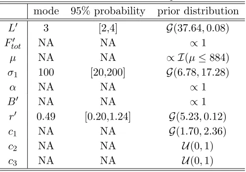
Thus, prior distributions are constructed based on our prior knowledge about where the param-eters should lie. Non-informative priors are employed where we do not have any prior information at all. The belief we have before we undertake the analysis in Section 6 is summarised in Table 1. From the observations we conclude thatL′ _{should be around 3 and probably between 2 and 4. We}

have the option to give more weight to the value of 3 and less weight as we move away from that value. Hence, we assume thatL′ _{∼ G}(37.64,0.08) which will give a 95% probability between 2 and 4 with mode at 3. For the total non-thermal energy _F′

tot we do not have any information at all, therefore _F′

tot ∝1.

We assume that the flare observations are from the cooling phase of the temperature profile; from the highest temperature lines downwards, the temperature drops continually. Thus, it is very likely that the main flare energy release will occur at most up until the first observation. For this reason we choose the mean of the non-thermal heat flux (µ) to have an upper limit at the lower error bar of the first observation (which is 884 s after the beginning of the observational period). Since we do not have any other belief about giving weights to any specific values we assume

µ _{∝ I}(µ_≤ 884), where _I(_·) is the indicator function (see Section 3.1). Also, σ1 ∼ G(6.78,17.28)

will give 95% probability for the one standard deviation of the heating function to be between 20 and 200 with mode at 100. Since we do not not have any knowledge about the background heating, we can assume an improper prior,e.g. π(B′)_∝1. In Section 6.2 we use_G(1.70,2.36) as a prior for

c1 and U(0,1) prior forc2, c3. The prior for c1 will give ∼99.90% probability for values below 20

and those forc2 andc3 come naturally as they will impose an upper limit of one, without favouring

any values below unity. Note that the prior for c2 can be conservative, as there might be evidence

that this number is close to the value 0.87 (Klimchuk et al. 2008).

For the radius of the loop as observed in Figure 1 from Raftery et al. (2009), we assume that the ratio R = _Lr′′ is probably 1/6. It is certainly no more than 1/2; so we give the ratio a 99.73%

probability to be inside the interval [0,0.5]. For this reason we have R _{∼ G}(6.03,0.03). Since

r′ ₌_R_×_L′ _and _{R, L}′ _{have known prior distributions, we can simulate the prior distribution of} _r′

(8)

Since we do not have any prior information regarding theα parameter, it would be preferable to give it an uninformative prior just as with B′_{. However, the fact that it is the “important”}

parameter of the analysis (if we want to test the hypotheses Hi, i= 0, . . . ,3) it has been given an informative prior, otherwise this would lead to Bartlett’s paradox (Lindley 1957; Bartlett 1957). Thus, a probability density function that will give a 50% probability forα <1 and a 50% probability for α >1 was chosen. For the H0 hypothesis (α 6= 1), this probability density function will be of

the form:

π(α) =

(

0.5, 0< α <1

0.5 exp(1₋α), α >1;

for theH2 hypothesis (α >1),π(α) = exp(1−α); and for theH3 hypothesis (α <1),α∼ U(0,1).

As far as the true time is concerned we can assume that it is normally distributed about the observed time with standard deviation obtained from the time error bars.

Our last assumption involves the initial values of the temperature, density and emission mea-sure. For this, we assume the pre-flare conditions to have an upper limit of 0.5 MK, 6 _×107 cm−3

and 4 _× 1043 _cm−3 _{respectively (Raftery et al. 2009). Since the non-thermal heating rate is}

al-most zero in the beginning, then because of Equation (1), the dominant heat input will be the background heating rate. Hence, these upper limits can indirectly serve as an upper limit to the background heating rate.

5. Model Comparison Methods

Model comparison methods using Bayesian statistics are reviewed in great detail in Clyde et al. (2007). An excellent description of how Bayes factor is applied in several problems can be found in Kass & Raftery (1995) and Raftery (1996). The key value for estimating the Bayes factor is to calculate the marginal density function:

p(D_|Hk) =

Z

P

p(D_|P)π(P)dP,

where Hk is the hypothesis (model) under consideration, p(D|P) is the likelihood function and

π(P) is the prior distribution. Basically, the marginal distribution is nothing more than the belief that we have about the data after we have integrated all the parameters, for the specific model under consideration. Then, the Bayes factor is given by:

BF01= p( D_|H0) p(D_|H1)

, (2)

for testing two hypotheses (H0 and H1). From Equation (2) it is clear that if BF01 ≫ 1 there

is more evidence in favour the H0 hypothesis, if BF01 ≪ 1 there is more evidence in favour the H1 hypothesis, whereas if BF01≈1 the data do not favour either model (but see Kass & Raftery

(9)

they are very difficult to calculate analytically, we will turn to numerical methods. In this paper we employ the two-stage sampler described in Adamakis et al. (2008).

We also employ the Akaike Information Criterion (AIC), proposed by Akaike (1974), and the Bayesian Information Criterion (BIC), proposed by Schwarz (1978). AIC propose to choose the model that minimises:

AIC =₋2(log maximised likelihood) + 2λ,

whereas the latter chooses the model that minimises:

BIC =₋2(log maximised likelihood) +λlogn,

whereλis the number of the parameters and nis the number of the data-points.

6. Results

The analysis can be separated into three crucial questions:

1. Which of the Half Gaussian and Full Gaussian functions fits better to the data we have?

2. Which of the thermal and non-thermal heat fluxes is dominant?

3. Should the ci values remain fixed or should they be free parameters?

The second question is the most important regarding the physics of the system. The other two questions are associated more with the statistical analysis. Nevertheless, they can indirectly affect which heat flux is most dominant because they contain relevant parameters. The estimations of the marginal densities of the different models that are shown in Figure 1 are presented in Table 2. For all the statistical models we have assumed that the mean energy of the accelerated (non-thermal) electrons impinging the chromosphere is_E = 15 keV. Different values of_Edo not have a large effect on the temporal profiles.

(10)

6.1. ci Fixed

6.1.1. Model selection

The ci parameters are fixed at c1 = 4, c2 = 0.87, c3 = 0.72 due to an acceptable overall

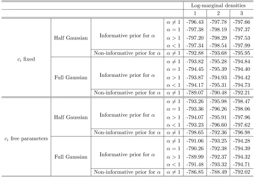
agreement with 1D HD simulations (Raftery et al. 2009; Klimchuk et al. 2008). From Table 2 and with a non-informative prior for α we can derive that the Bayes factor between the Full Gaussian and the Half Gaussian heating function is 42.10 using the Importance sampling estimator. This provides “strong” evidence in favour of the Full Gaussian, according to the table in Kass & Raftery (1995). By looking the results for the H0 :α6= 1 hypothesis, there is “positive” evidence in favour

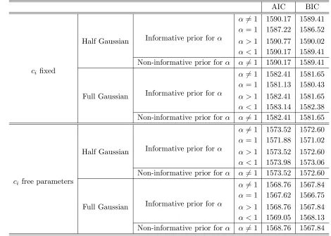
of the Full Gaussian. The information criteria agree with this conjecture (see Table 3). Note that the values for AIC and BIC are the same for the hypotheses α ₆= 1 because the information criteria do not depend on the priors. From this, we can conclude that there is enough evidence to support that the Full Gaussian function for the heating profiles is much more adequate than the Half Gaussian, at least for the particular data-set under analysis.

In order to distinguish between the thermal and non-thermal heat fluxes, let us focus on the results from Table 2 with the informative prior forα. Roughly speaking, the model with the largest marginal density will provide evidence of its favour among a given class of models. Using the Full Gaussian we conclude that the evidence we get is “not worth more than a bare mention” for any hypothesis (α >1, α <1, α = 1). We reach the same conclusion for the Half Gaussian as all the marginal probability densities are almost the same. On the other hand the information criteria select theα= 1 hypothesis for both Gaussian functions. This time, the model that minimises the information criteria can be proven more useful among a given set of models.

Thus, if we had to choose one of the three hypotheses, we would have chosenα= 1, i.e. equal amount of thermal and non-thermal heat input, as there is lack of evidence to support a more complicated statistical model. Since the Full Gaussian is more preferable than the Half Gaussian we will choose to adopt the Full Gaussian results for estimating the parameters.

6.1.2. Parameter estimation

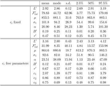
The results of this analysis with non-informative prior for α can be viewed in Table 4. We estimate the mean of L to be 29.20 Mm, which is close to what was used by Raftery et al. (2009) (i.e. 30 Mm). The mean total non-thermal heat flux is calculated around 79.83_×109 _{ergs cm}−2_,

while mean time for the peak of this function is 853.5 s after the beginning of the flare. For the α

(11)

that is misused in astrophysics and can lead to false conclusions. More discussion about this is presented in Section 7.

The first column of Figure 2 shows the best fit of the parameters regarding the posterior distributions. Even by eye we can distinguish between the Full Gaussian and the Half Gaussian function. As previously discussed, introducing a prior distribution for theαparameter, while there is no prior information, will create a bias. This is the price we have to pay in order to address Question 2. However, the prior we employed seems reasonable as it provides 1/2 probability for 0 < α <1 and, subsequently, 1/2 probability for α >1. In order to see how different the results are, both with and without prior information for theα parameter, then we compare Table 4 with the respective table we get from the analysis where prior information forα is imported. From that we can conclude that all the parameters have almost the same posterior distributions, apart from the _Ftot parameter. Especially for this parameter, a 95% highest posterior density interval2 _will

give [51.51,544.56] with informative prior forαand [2.11,171.90] with non-informative prior forα.

6.2. ci Parameters

6.2.1. Model selection

We follow the same procedure as in Section 6.1.1 in order to derive the models that best describe the data. Regarding which of the two non-thermal heat fluxes is more dominant, there is no question that the Full Gaussian is more preferable as can be seen from Table 2 (the Bayes factor in favour of the Full Gaussian is 142.54 with non-informative prior for α, according to the Importance sampling estimator). This can be characterised as “very strong” evidence in favour of the Full Gaussian. The same preference for the Full Gaussian function can be derived by comparing the log-marginal densities for α ₆= 1 with informative prior for α. From Table 3 the information criteria are in agreement with this. Therefore, the fact that we included theci as free parameters, did not alter the outcome comparing to the analysis in Section 6.1.1 where the ci are fixed.

Using an informative prior for α and the Full Gaussian non-thermal heat flux, it can be concluded from Table 2 that the α >1 hypothesis is slightly better than the other two. But this evidence is not that strong and it can be characterised as “not worth more than a bare mention”. For the Half Gaussian model the same picture is obtained: the data we have cannot distinguish which of the thermal or non-thermal heat fluxes is more dominant, if either. The information criteria (see Table 3) choose the Full Gaussian distribution and α = 1. Therefore, if we had to choose a hypothesis we would go for equal amount of thermal and non-thermal heat flux (α= 1).

2_{A 95% highest posterior density interval of a parameter leaves 95% probability for the parameter to be inside}

(12)

6.2.2. Parameter estimation

All the estimations from the posterior distributions of the parameters can be viewed in Table 4, using the Full Gaussian function. We estimate the mean of L to be 31.6 Mm, the mean of the total non-thermal heat flux is 31.99_×109 _{ergs cm}−2_{, the mean time for the peak of this function}

864.6 s after the beginning of the flare, the mean of the standard deviation of the Full Gaussian is 92.6 s, the mean of theαparameter is 23.51, the mean background heating rate is 0.12_×10−5 _ergs

cm−3 _s−1 _{and the radius of the loop is 6}_._{7 Mm.}

Regarding theci ratios, the mean of the ratio between the radiative loss rate of the transition and the corona (c1) is 2.07, the mean of the ratio between the average coronal temperature and

the apex temperature (c2) is 0.86 and the mean of the ratio between the coronal base temperature

and the apex temperature (c3) is 0.75. Once again, we should bear in mind that although the

estimation forα is greater than unity (23.51) with non-informative prior, a more detailed analysis shown in Section 6.2.1 suggests that we cannot distinguish which of the thermal or non-thermal heat fluxes is more dominant. Furthermore, assuming informative prior for α, α is greater than unity with probability 57.13% . The second column of Figure 2 shows the best fit of the parameters regarding the posterior distributions for both the Full and Half Gaussian functions.

As in Section 6.1.2, we want to check the sensitivity of the analysis regarding the prior in-formation for α. Comparing Table 4 with the respective table we get when we use informative prior for α, then the only difference worth mentioning is the _F′

tot parameter which will give a 95% highest posterior density interval [37.33,318.38] for informative prior for α and [3.26,119.65] for non-informative prior for α.

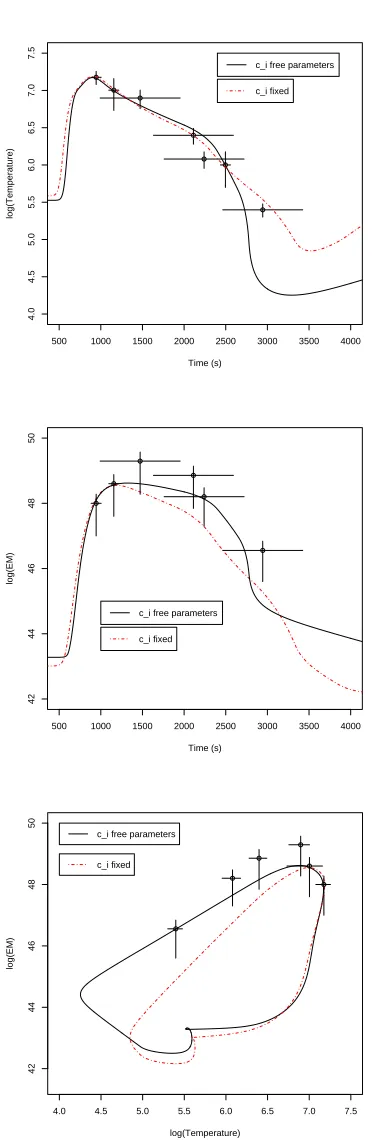
6.3. Comparison Between the Hypotheses: ci Fixed and ci Free Parameters.

Considering the non-thermal heat flux, both of the two hypotheses (ci fixed andci free param-eters) propose the Full Gaussian statistical model. However, none of them can distinguish which of the two heating mechanisms is dominant (if any). Regarding Question 3, from Table 2 we reach dif-ferent conclusions depending on the estimation method for the marginal distribution: Importance sampling do not seem to favour any hypothesis, but the other two methods favour the hypothesis

ci free parameters. However, the information criteria (Table 3) clearly choose the hypothesisci free parameters. This indicates that the values introduced forciwhen they are fixed are not very good, in terms of maximising the likelihood function. The information added whenci are free parameters is higher than the price we have to pay for introducing three additional parameters.

(13)

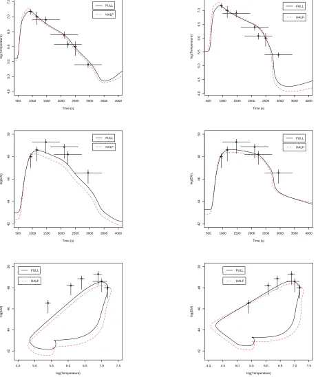
measure values than the temperature values. The fact that there are better values for ci than 4, 0.87 and 0.72 is even more clear in the third row where temperature is plotted against emission measure.

7. Discussion

In order to reveal the mysteries of the Sun, we can break down our investigations into three major stages: (i) constructing theoretical models, (ii) gathering observations, and (iii) applying a statistical analysis in order to compare different statistical models and/or to restrict the parameters of the models. All of them are of equal importance and give us confidence in our results.

Making inference alone from the mean or mode of Table 4 is of utmost criticism. For model comparison purposes the 95% credible interval is more robust. However, even with the 95% credible interval we can not compare with the α = 1 hypothesis. Also, we do not directly include the likelihood function in our calculations. On the other hand, model comparison techniques like AIC and BIC take into account the likelihood function but ignore the spread of the parameter distributions. However, model comparison techniques using Bayesian statistics (e.g. Bayes factor) take into account both the spread of the parameter posterior distributions and the information of the likelihood function.

In this paper, temperature and emission measure profiles produced by the EBTEL model were compared with solar flare observations. The data distribution, the parameter space and the priors employed in this analysis were described in great detail. The form of thermal and non-thermal heat input is much better described using Full Gaussian energy profile than Half Gaussian, which is what Raftery et al. (2009) also used. This is not surprising as the heating function is expected to mimic the X-ray profile, which is often found to be Gaussian-like.

Apart from choosing which function was more appropriate for the data-set we analysed, we were also interested in determining which of the thermal or non-thermal heat fluxes was more dominant. The data obtained were not able to provide an answer with great confidence. More data-points may be required in order to address this question. However, this result implies that both thermal and non-thermal heating mechanisms are almost equally important during the flaring process. Although, this is in agreement with Raftery et al. (2009), we fully recommend a proper treatment of statistics as we may be led to fallacious results as in Ugarte-Urra et al. (2005), which were discovered in Adamakis et al. (2008).

(14)

The fact that the Bayes factor is not so decisive in choosing between the hypotheses ci fixed or free parameters is partially an outcome of the conservative prior distributions we have chosen for theci parameters (see Section 4). If we had added more information in the prior distribution of

c2, say U(0.5,1) or even better the Beta distributionB(38.49,5.75), this would have been in favour

of the ci parameters hypothesis. However, since we do not know anything about these values in advance, it is better to have them as free parameters and let the simulation decide upon these values. More improved estimations for these parameters can be seen from the mean or mode of Table 4 (for the particular data-set we analyse).

Finally, an obstacle presented in this analysis was that of constraining the profiles produced by the EBTEL model. For example, we might not want to restrict the initial values of temperature, density and/or emission measure profiles. This might produce model profiles that are closer to the data profiles, but the initial values might take exceptionally high numbers. For example, we had undertaken the same analysis without fixing the initial values of temperature, density and emission measure. This resulted in model profiles with initial temperatures of 3 MK, initial electron density of 500_×107_cm−3 _{and initial emission measures of 3}_×₁₀47_cm−3_{. This was because the background}

heating rate was three orders of magnitude higher than that in Table 4. Apart from unrealistic estimations of the parameters of interest, this could have also have led to unreliable Bayes factor estimations with false conclusions regarding the three posed questions in the beginning of Section 6. Naturally, the quality of the output of the analysis is dependent of the quality of the input.

Apart from improved statistical techniques, of equal importance is that improvement upon the observations should be made. This means that future missions with new instrumentation should provide data-sets with a large enough number of observations in order to distinguish between different heating mechanisms. The data-set under consideration provided information only upon the decay phase of the temporal evolution. However, a better time resolution for the rise phase of the temperature will be needed in order to provide a better estimate for the form of thermal/non-thermal heat flux. And of course, a large sample of solar flares will be required.

An assumption made by Raftery et al. (2009) was that the thermal and non-thermal fluxes have the same form, based on a lack of information on the thermal distribution. However, it would be interesting to test fluxes of different forms that do not depend on each other. Additionally, a further improvement in the EBTEL model is required regarding the non-thermal heat flux, as it is efficient for gentle chromospheric evaporation but suffers from inadequately representing explosive chromospheric evaporation. In addition, several other forms of heating input, like proton beams, could be included in an attempt to make the model more realistic.

(15)

REFERENCES

Adamakis, S. 2009, PhD thesis, University of Central Lancashire

Adamakis, S., Walsh, R., & Morton-Jones, T. 2008, Constraining Coronal Heating: Employing Bayesian Analysis Techniques To Improve the Determination of Solar Atmospheric Plasma Parameters, [arXiv:0807.4209]

Aitken, C. & Taroni, F. 2004, Statistics and the Evaluation of Evidence for Forensic Scientists (John Wiley and Sons Ltd.)

Akaike, H. 1974, IEEE Transactions on Automatic Control, 19, 716

Aschwanden, M. 2005, Physics of the Solar Corona: An Introduction with Problems and Solutions (Springer Praxis Books/Astronomy and Planetary Sciences)

Bartlett, M. S. 1957, Biometrika, 44, 533

Berkson, J. 1950, Journal of the American Statistical Association, 45, 164

Carlin, B. & Louis, T. 2000, Bayes and Empirical Methods for Data Analysis (Chapman and Hall/CRC)

Chen, M.-H., Shao, Q.-M., & Ibrahim, J. 2000, Monte Carlo Methods in Bayesian Computation (Springer-Verlag New York, Inc.)

Clyde, M., Berger, J., Bullard, F., et al. 2007, in Statistical Challenges in Modern Astronomy IV, ed. G. J. Babu & E. D. Feigelson (ASP Conference Series, Vol. 371), 224–240

Henderson, R., Morton-Jones, A., & McKnespiey, P. 2000, Applied Statistics, 49, 563

Jaynes, E. 1991, Straight Line Fitting – A Bayesian Solution [Internet] (Updated 21 April 1999), Technical Report. Available at http://bayes.wustl.edu/etj/node2.html [Accessed 22 March 2008]

Kass, R. E. 1993, Statistician, 42, 551

Kass, R. E. & Greenhouse, J. 1989, Statistical Science, 4, 310

Kass, R. E. & Raftery, A. 1995, Journal of the American Statistical Association, 90, 773

Kass, R. E. & Wasserman, L. 1996, Journal of the American Statistical Association, 91, 1343

Klimchuk, J., Patsourakos, S., & Cargill, P. 2008, The Astrophysical Journal, 682, 1351

Lindley, D. V. 1957, Biometrika, 44, 187

(16)

Milligan, R., Gallagher, P., Mathioudakis, M., et al. 2006a, The Astrophysical Journal, 638, L117

Milligan, R., Gallagher, P., Mathioudakis, M., & Keenan, F. 2006b, The Astrophysical Journal, 642, L169

Raftery, A. E. 1996, in Markov Chain Monte Carlo in Practice, ed. W. Gilks, S. Richardson, & D. Spiegelhalter (Chapman and Hall), 163–188

Raftery, C., Gallagher, P., Milligan, R., & Klimchuk, J. 2009, Astronomy & Astrophysics, 494, 1127

Schwarz, G. 1978, Annals of Statistics, 6, 461

Ugarte-Urra, I., Doyle, J. G., Walsh, R. W., & Madjarska, M. S. 2005, Astronomy & Astrophysics, 439, 351

Winsor, C. 1946, Biometrics Bulletin, 2, 101

(17)

[image:17.612.194.413.95.695.2]

(18)

500 1000 1500 2000 2500 3000 3500 4000 4.5 5.0 5.5 6.0 6.5 7.0 7.5 Time (s) log(Temperature) FULL HALF

500 1000 1500 2000 2500 3000 3500 4000

4.0 4.5 5.0 5.5 6.0 6.5 7.0 Time (s) log(Temperature) FULL HALF

500 1000 1500 2000 2500 3000 3500 4000

42 44 46 48 50 Time (s) log(EM) FULL HALF

500 1000 1500 2000 2500 3000 3500 4000

42 44 46 48 50 Time (s) log(EM) FULL HALF

4.5 5.0 5.5 6.0 6.5 7.0 7.5

42 44 46 48 50 log(Temperature) log(EM) FULL HALF

4.0 4.5 5.0 5.5 6.0 6.5 7.0 7.5

[image:18.612.74.536.133.681.2]

42 44 46 48 50 log(Temperature) log(EM) FULL HALF

Fig. 2.—: Temperature evolution (first row), emission measure evolution (second row) and tem-perature against emission measure (third row) using the EBTEL model that best reproduced the observations (maximised the posterior distributions). Solid lines represent the fit from the Full Gaussian function for the thermal and non-thermal heat inputs, whereas dashed lines represent the fit from the Half Gaussian function. For all the curvesnon-informativeprior forαwas employed.

First column depicts solutions using the ci fixed, whereas second column depicts solutions from ci

(19)

500 1000 1500 2000 2500 3000 3500 4000

4.0

4.5

5.0

5.5

6.0

6.5

7.0

7.5

Time (s)

log(Temperature)

c_i free parameters

c_i fixed

500 1000 1500 2000 2500 3000 3500 4000

42

44

46

48

50

Time (s)

log(EM)

c_i fixed c_i free parameters

4.0 4.5 5.0 5.5 6.0 6.5 7.0 7.5

42

44

46

48

50

log(Temperature)

log(EM)

c_i free parameters

[image:19.612.209.396.109.679.2]

c_i fixed

(20)

[image:20.612.183.432.324.498.2]

Table 1:: Prior belief about the parameters. mode 95% probability prior distribution

L′ ₃ _[2,4] _G₍₃₇_.₆₄_,₀_.₀₈₎

F_tot′ NA NA _∝1

µ NA NA _{∝ I}(µ_≤884)

σ1 100 [20,200] G(6.78,17.28)

α NA NA _∝1

B′ _NA _NA _∝₁

r′ 0.49 [0.20,1.24] _G(5.23,0.12)

c1 NA NA G(1.70,2.36)

c2 NA NA U(0,1)

(21)

[image:21.612.69.570.285.635.2]

Table 2:: Logarithmic marginal densities estimations under several hypotheses, using the EBTEL model to compare with temperature and emission measure profiles (Raftery et al. 2009). This table produces results for both ci fixed and free parameters for comparison tests. The logarithmic marginal densities are estimated using: 1: Laplace method with posterior covariance matrix, 2: Laplace method with robust posterior covariance matrix, 3: Importance sampling estimation with the probability density from stage 1 as the additional probability density (Adamakis et al. 2008).

Log-marginal densities

1 2 3

α₆= 1 -796.43 -797.78 -797.66

α= 1 -797.38 -798.19 -797.37 Half Gaussian Informative prior for α α >1 -797.20 -798.29 -797.53

α <1 -797.34 -798.54 -797.99 Non-informative prior forα α₆= 1 -792.88 -793.68 -795.95

ci fixed _α₆_{= 1} _-793.82 _-795.28 _-794.84

α= 1 -794.45 -795.39 -794.40 Full Gaussian Informative prior for α α >1 -793.87 -794.93 -794.42

α₆= 1 -793.26 -795.98 -798.47

α= 1 -793.36 -796.26 -798.06 Half Gaussian Informative prior for α α >1 -794.07 -795.91 -797.96

ci free parameters _α₆_{= 1} _-791.06 _-793.25 _-794.28

α= 1 -790.26 -792.38 -794.39 Full Gaussian Informative prior for α α >1 -789.99 -792.37 -794.32

(22)

[image:22.612.66.536.265.600.2]

Table 3:: Information criteria for comparison between temperature/emission measure profiles pro-duced using the EBTEL model and observations (Raftery et al. 2009). This table produces results for both ci fixed and free parameters for comparison tests.

AIC BIC

α₆= 1 1590.17 1589.41

α= 1 1587.22 1586.52 Half Gaussian Informative prior for α α >1 1590.77 1590.02

α <1 1590.17 1589.41 Non-informative prior forα α₆= 1 1590.17 1589.41

ci fixed _α₆_{= 1} _1582.41 _1581.65

α= 1 1581.13 1580.43 Full Gaussian Informative prior for α α >1 1582.41 1581.65

α₆= 1 1573.52 1572.60

α= 1 1571.88 1571.02 Half Gaussian Informative prior for α α >1 1573.52 1572.60

ci free parameters _α₆_{= 1} _1568.76 _1567.84

α= 1 1567.62 1566.75 Full Gaussian Informative prior for α α >1 1568.76 1567.84

(23)

[image:23.612.127.485.285.565.2]