Characterising the Human Auditory System using a Linear Least Squares System Identification Approach

Characterising the Human Auditory

System using a Linear Least-Squares

System Identification Approach

Denis P. Drennan, BEng, MEng

Under the supervision of

Dr. Edmund C. Lalor

A dissertation submitted to the

University of Dublin, Trinity College

in fulfilment of the requirements for the degree of

Doctor of Philosophy

16

August 2019

ii

Declaration

I, Denis Drennan, confirm that this thesis has not been submitted as an exercise for a degree at this or any other university and is entirely my own work.

I agree to deposit this thesis in the University's open access institutional repository or allow the Library to do so on my behalf, subject to Irish Copyright Legislation and Trinity College Library conditions of use and acknowledgement.

Signed,

______________________ Denis P. Drennan

iii

Summary

Disabling hearing loss affects many millions of people around the world. Early identification and suitable interventions, e.g., the provision of hearing aids, cochlear implants, etc., can help but are limited by the methods currently used to assess hearing function. Hearing function can be assessed in one of two ways: using either subjective or objective methods. Subjective methods rely on the behavioural response to sound, while objective methods rely on the physiological response to sound. While subjective methods such as pure tone audiometry (PTA) have played an important role in hearing assessment for decades, they are generally limited to simple detection tasks, e.g. detecting pure tones in quiet, and provide little indication as to the source of any deficit. While some objective measures such as the auditory evoked potential (AEP)—a transient electrophysiological response to sound—can provide more detailed neurophysiological information, they are often restricted by the need to use simple discrete stimuli such as clicks or tone-bursts, which are arguably not that representative of everyday sounds.

iv this thesis is to develop and appraise new methodological approaches that facilitate the use of TRF estimation in the study and assessment of low-level (sensory) auditory processing.

In Chapter 4, two approaches for indexing low-level processing along the auditory pathway are introduced over two experiments: Experiment 1 and 2. Experiment 1 is an initial exploratory attempt to derive responses along the auditory pathway to click trains, i.e., sequences of click stimuli—the classic stimuli of auditory research. Experiment 2 is a more thorough attempt to derive responses along the auditory pathway to amplitude modulated (AM) broadband noise (BBN), using a novel efficient TRF estimation approach. Considerations of stimulus type, stimulus representation, i.e., what stimulus feature to use and how to represent it in the analysis, and computational efficiency are discussed, and the neural underpinnings of the derived responses investigated through comparisons with their canonical counterparts, i.e., AEPs, elicited using chirp trains.

In Chapter 5, a novel TRF estimation approach for objectively determining hearing thresholds, i.e., the lowest levels at which certain sounds can be heard in quiet, using multiplexed, i.e., multiple, mixed, AM tones (AMTs) is presented. Considerations of stimulus type, stimulus representation, and modelling approach are discussed, and the performance of this approach evaluated through comparisons with thresholds recovered using PTA, in both normal hearing and hearing loss populations.

In Chapter 6, several novel stimulus representations are presented with the view of enhancing response derivation using TRF estimation. The importance and benefits of taking certain neurophysiological properties of the human auditory system into account when designing stimulus representations are discussed and then quantified through comparisons with other models derived using more standard stimulus representations.

v

Acknowledgements

This thesis would not have been possible without the support of several people. Therefore, I would like to thank:

Ed, for your constant support and guidance throughout the PhD. I have learned a lot from you over the years. Thank you for making it both interesting and fun.

Richard, for all your kind help and advice.

Mick, for getting me set up in the beginning, and for your time and patience even though you were so busy completing your own PhD.

Kevin, for all your help, particularly with MAMTA. It is very much appreciated. Other past and current members of the Lalor Lab: Ger, Jim, Gio, Andy, Nate, Aaron, Adam, Emily, Michael, Aisling, Joyce, Kathryn, Shyantony, and Lauren. Thank you for all your helpful feedback and advice, and for making the Lalor Lab such a nice place to work.

Ter, for all the consultation and comic relief. This would have been a very different experience without you. Thanks for everything.

Other past and current members of the Reilly Lab: Céline, Isabelle, Martin, Alejandro, Brendan, Niamh, Saskia, Ciara, Surbhi, Shruti, Clodagh, and Eugene. Thank you for making these last few years so memorable.

Ross, for getting me started on this road many years ago, and for your support throughout. I have learnt a lot from you over the years, for which I am very grateful.

vi Caroline and Brendan, for all your help with patient recruitment, audiological testing, and for all the good times.

Everyone else in Neuromod Devices for making it a wonderful place to work over the last few years.

My parents Thos and Angela, for your constant love and support, and for instilling within me a strong work ethic, through your own example.

My brother Tom for your friendship and advice, and for feeding my intellectual curiosity outside of the PhD.

Marie, for your love, support, and patience throughout what was a challenging few years at the beginning of our relationship. I will always be grateful.

All the subjects who generously volunteered their time to participate in these studies.

This research was kindly supported by the Irish Research Council (IRC) and Science Foundation Ireland (SFI).

D

P

D

vii

Publications Arising from this Thesis

Journal Articles

• Drennan DP, Lalor EC (2019). Cortical tracking of complex sound envelopes: modeling the changes in response with intensity. eNeuro, ENEURO.0082-19.2019.

Journal Articles in Preparation

• Drennan DP, Lalor EC (in prep.). Indexing the Human Auditory Processing Hierarchy: Considerations of Stimulus Type, Stimulus Representation, and Computational Efficiency.

Conference Poster Presentations

• Drennan DP, Lalor EC. Improved Modelling of Auditory Responses to Amplitude Modulation using Multivariate Representations of Amplitude. Auditory EEG Signal Processing 2018, Leuven, Belgium.

• Drennan DP, Lalor EC. A System Identification Approach for Rapid Characterization of the Human Auditory System. Society for Neuroscience 2016, San Diego, USA.

1

Table of Contents

Declaration ... ii

Summary ... iii

Acknowledgements ... v

Publications Arising from this Thesis ... vii

Journal Articles ... vii

Journal Articles in Preparation ... vii

Conference Poster Presentations ... vii

Table of Contents ... 1

List of Figures ... 5

List of Tables ... 7

Glossary of Abbreviations ... 8

Chapter 1. Introduction ... 10

Background ... 10

Aims ... 12

Thesis Outline ... 13

Chapter 2. Electrophysiology of Human Auditory Processing ... 15

Anatomy and Physiology of Human Auditory Processing ... 15

Peripheral Auditory System ... 15

Central Auditory System... 18

Auditory Cortex ... 19

Pathophysiology of Human Auditory Processing ... 20

Conductive Hearing Loss ... 20

2

Hidden Hearing Loss ... 20

Electrophysiology of Low-Level Human Auditory Processing ... 21

Electroencephalography ... 21

Electrophysiological Measures of Low-Level Human Auditory Processing .... 22

Auditory Evoked Potential ... 22

Recovering Auditory Evoked Potentials ... 23

Chapter 3. Temporal Response Function Estimation ... 26

Introduction ... 26

Forward Models ... 28

Backward Models ... 28

Regularisation ... 30

Model Fitting Procedure ... 31

Stimulus Representation ... 31

Interpretation ... 33

Relationship to AEP ... 34

Chapter 4. Indexing the Human Auditory Processing Hierarchy: Considerations of Stimulus Type, Stimulus Representation, and Computational Efficiency ... 35

Experiment 1 ... 35

Introduction ... 35

Materials and Methods ... 36

Subjects ... 36

Stimuli ... 37

Experimental Procedure ... 37

EEG Acquisition ... 38

EEG Preprocessing ... 38

Temporal Response Function Estimation ... 38

Results ... 39

3

Experiment 2 ... 41

Introduction ... 41

Materials and Methods ... 41

Subjects ... 41

Stimuli ... 41

Experimental Procedure ... 43

EEG Acquisition ... 44

EEG Preprocessing ... 44

Temporal Response Function Estimation ... 44

AM BBN Stimulus Representations ... 45

Modelling Approaches ... 46

Results ... 48

Validating our Choice of Stimulus Representation ... 48

Evaluating the Reduced and Variable Sampling Rate Responses ... 50

Comparing the Variable Sampling Rate Full-Range Multiple-Latency Response to Canonical Responses ... 53

Discussion ... 57

Chapter 5. MAMTA: Multiplexed Amplitude Modulated Tone Audiometry... 61

Introduction ... 61

Materials and Methods ... 63

Subjects ... 63

Stimuli ... 63

Experimental Procedure ... 64

EEG Acquisition ... 65

EEG Preprocessing ... 65

Temporal Response Function Estimation ... 66

Stimulus Representation ... 66

4

Results ... 67

Examining the Relationship between Reconstruction Accuracy and Hearing Loss 67 Using Reconstruction Accuracies to Determine Hearing Thresholds ... 70

Discussion ... 74

Chapter 6. Stimulus Dependent Modelling of the Cortical Tracking of Complex Sound Envelopes 77 Introduction ... 77

Materials and Methods ... 78

Subjects ... 78

Stimuli ... 79

Experimental Procedure ... 79

EEG Acquisition ... 81

EEG Preprocessing ... 82

Temporal Response Function Estimation ... 82

Amplitude-Binned Envelope Stimulus Representation ... 82

Other Stimulus Representations ... 83

Model Comparison... 84

Results ... 86

Channel Selection ... 86

Individual Model Comparisons... 86

Combined Model Comparisons ... 90

Discussion ... 93

Chapter 7. General Discussion ... 95

Introduction ... 95

Low-Level Assessment ... 95

Low- and High-Level Assessment ... 97

Decoding ... 97

Summary and Conclusions ... 98

5

List of Figures

Figure 2.1: Peripheral Auditory System ... 17

Figure 2.2: Central Auditory System ... 18

Figure 2.3: Auditory Cortex ... 19

Figure 2.4: ABR, MLR, and LAEP ... 23

Figure 2.5: Time-Domain Averaging ... 25

Figure 3.1: TRF Estimation ... 27

Figure 4.1: Example Segments of the Stimuli Used in This Experiment ... 37

Figure 4.2: Grand Average Click Train vs. Grand Average Chirp Train LAEPs ... 39

Figure 4.3: Example Segments of the Stimuli used in This Experiment. ... 43

Figure 4.4: Time-lag Differences and Equivalent Reduced and Variable Sampling Rates ... 48

Figure 4.5: Narrowband, Broadband, and Gammachirp Envelope ABRs ... 49

Figure 4.6: ABRs Derived using the FSFR, FSRR, RSRR, and VSFR Approaches ... 51

Figure 4.7: MLRs Derived using the FSFR, FSRR, RSRR, and VSFR Approaches ... 52

Figure 4.8: LAEPs Derived using the FSFR, RSFR, and VSFR Approaches ... 53

Figure 4.9: Comparison of VSFR and 20.1 Hz LS-Chirp train ABRs. ... 55

Figure 4.10: Comparison of VSFR and 12.3 Hz LS-Chirp train MLRs. ... 56

Figure 4.11: Comparison of VSFR and 1.0 Hz LS-Chirp train LAEPs. ... 57

Figure 5.1: Example Segments of the Calibrated AMTs Used in This Study ... 64

Figure 5.2: Uncompensated Global Relationship between Reconstruction Accuracy and Hearing Loss. ... 68

6 Figure 5.4: Compensated Global Relationship between Reconstruction Accuracy and Hearing

Loss. ... 70

Figure 5.5: Scatter Plots of Compensated Reconstruction Accuracies against PT Thresholds at Each Frequency ... 71

Figure 5.6: Representative Reconstruction Accuracy Profiles for the Moving-Threshold Approach ... 73

Figure 6.1: Example Segments and Properties of the Stimuli Used in This Study ... 81

Figure 6.2: Example Segments of Some of the Stimulus Representations Used in this Study 84 Figure 6.3: Prediction Accuracies for the AM BBN Dataset... 87

Figure 6.4: Analysis of Amplitude-Dependent Changes for the AM BBN Dataset. ... 89

Figure 6.5: Prediction Accuracies for the Speech Dataset ... 90

Figure 6.6: Analysis of Amplitude-Dependent Changes for the Speech Dataset. ... 91

7

List of Tables

8

Glossary of Abbreviations

AB Amplitude-Binned

ABR Auditory Brainstem Response ADJAR Adjacent Response

AEP Auditory Evoked Potential

AM Amplitude Modulated

AMT Amplitude Modulated Tone ASSR Auditory Steady-State Response BBN Broadband Noise

cABR Complex Auditory Brainstem Response CLAD Continuous Loop Averaging Deconvolution

dB Decibel

EEG Electroencephalography EMG Electromyography EOG Electrooculography

FAB Frequency- and Amplitude-Binned

FB Frequency-Binned

fMRI Functional Magnetic Resonance Imaging FSFR Full Sampling Rate Full Range

FSRR Full Sampling Rate Reduced Range GFP Global Field Power

9 LAEP Late Auditory Evoked Potential

LS Level-Specific / Least-Squares

MAMT Multiplexed Amplitude Modulated Tone

MAMTA Multiplexed Amplitude Modulated Tone Audiometry MEG Magnetoencephalography

MLR Middle-Latency Response MLS Maximum Length Sequence

MSAD Multiple-Rate Steady-State Deconvolution

peRETSPL Peak-to-Peak Equivalent Reference Equivalent Threshold SPL peSPL Peak-to-Peak Equivalent SPL

PT Pure-Tone

PTA Pure-Tone Audiometry QSD Q-Sequence Deconvolution

RSA Randomized Stimulation and Averaging RSFR Reduced Sampling Full Range

RSRR Reduced Sampling Rate Reduced Range SEM Standard Error of the Mean

10

Chapter 1.

Introduction

Background

According to the World Health Organisation (WHO) 466 million people worldwide have disabling hearing loss, 34 million of whom are children (WHO, 2018). Disabling hearing loss is defined in this context as hearing loss greater than 40 dB in the better hearing ear of adults, and greater than 30 dB in the better hearing ear of children (WHO, 2018). Early identification and suitable interventions, e.g., the provision of hearing aids, cochlear implants, etc., can help, but are limited by the methods currently used to assess hearing function.

Hearing function can be assessed in one of two ways: using either subjective or objective methods. Subjective methods rely on the behavioural response to sound, while objective methods rely on the physiological response to sound. One widely used subjective method is pure-tone audiometry (PTA; Bunch, 1923, 1922). With PTA, a subject is typically presented with short excerpts of a pure-tone (PT) at a fixed level and asked if they can hear it. The level is then adjusted in descending and ascending runs until the lowest level at which they can hear that tone, i.e., their hearing threshold for that tone, has been determined. This process is then repeated for the other frequencies being tested, until a full audiometric profile has been established (BSA, 2011).

11 et al., 1966). And so, there has been a growing interest for many years in the use of objective measures.

One widely used objective measure is the so-called auditory evoked potential (AEP). This is a transient electrophysiological response to brief sounds, recorded from the auditory system using electrodes placed on the scalp—a technique referred to as electroencephalography (EEG). AEPs show several characteristic voltage fluctuations known as waves at different latencies that can be linked with different processing stages along the auditory pathway. By examining the properties of these waves, one can hope to pinpoint the locus of hearing dysfunction in a quantitative and objective manner (Musiek et al., 1994). Like PTA, the AEP can also be used to determine hearing thresholds (Tyberghein and Forrez, 1971). Unlike PTA, it can be used to evaluate suprathreshold processing (Ruggles et al., 2011) and is suitable for use with young children or those with a diminished capacity to respond.

While these characteristics make the AEP a potentially attractive tool for assessing hearing function, it has traditionally had two major disadvantages. First, response recovery can be relatively slow as the signal-to-noise ratio (SNR) associated with it is poor—as most of the EEG recorded from the scalp is unrelated to the presented sound—and separate sets of stimuli and resulting EEG are required to assess each hierarchical processing stage (latency) of interest. Second, the AEP—like most objective measures—is typically elicited using simple discrete stimuli, like clicks or tone-bursts, but as the human auditory system has evolved to process a broad spectrum of sounds—from simple discrete stimuli such as the crack of a twig, to complex continuous stimuli such as speech—it would seem fitting that the approach used to interrogate this system be able to utilise such a wide variety of sounds.

While some methods have enabled measures to be recovered using more complex stimuli, e.g., the complex auditory brainstem response (cABR; Skoe and Kraus, 2010)—a transient electrophysiological response to short repeated syllables—the quasi-discrete, repeated nature of its elicitation, is unlikely to engage the kinds of high-level (cognitive) auditory processing commensurate with continuous natural speech. While other methods have enabled measures to be recovered using continuous stimuli, e.g., the auditory steady-state response (ASSR; Galambos et al., 1981)—an oscillatory electrophysiological response usually to regularly amplitude modulated (AM) sounds—this comes at the cost of any temporal resolution in the response, i.e., it is typically analysed in the frequency domain.

12 (TRF) estimation (Lalor et al., 2009). TRF estimation is a modelling approach, that tries to fit models that describe the relationship between a sensory input and neural response, i.e., it uses features of the observed inputs, e.g., auditory stimuli, and outputs, e.g., EEG, to mathematically estimate the intermediary, e.g., auditory, system response (TRF). As mentioned, the main advantage of this approach is that it can be used with almost any auditory stimuli while still retaining full temporal resolution in the response. For example, Lalor et al. (2009) showed that using TRF estimation, it is possible to derive low-level, i.e., sensory, auditory responses to quasi-periodic tone-bursts, AM tones (AMTs), and AM broadband noise (BBN), while Lalor and Foxe (2010) showed that it is possible to derive low-level auditory responses to continuous natural speech.

However, much of the work that has been done using this approach has been focused on high-level auditory processing, e.g., while studying the so-called cocktail party attention problem, i.e., the problem associated with attending to one speaker in a multi-speaker environment (O’Sullivan et al., 2015), as well as linguistic processing at the level of phonemes (Di Liberto et al., 2015) and semantics (Broderick et al., 2018). That was until recently, however, when Maddox and Lee (2018) modified the TRF estimation approach and showed that it is possible to derive low-level responses to continuous natural speech, from the entire auditory pathway simultaneously, i.e., not just from the auditory cortex as in Lalor and Foxe (2010). That is not to say that these two endeavours are entirely unrelated, however, indeed this finding may facilitate the study of interactions between high and low-level auditory processing, thus bridging the gap between these two bodies of work.

It would seem then that this approach holds a lot of potential for the study and assessment of low-level auditory processing—for which it remains relatively underexplored— and that any advances to that end, may benefit the study and assessment of high-level processing as well. As such, it represents an opportunity to move the field closer towards more diagnostically useful objective measures of hearing function along the auditory pathway.

Aims

13 1. To develop a novel TRF estimation approach for efficiently deriving low-level

responses from the entire auditory pathway.

2. To develop a novel TRF estimation approach for objectively determining hearing thresholds, and to pilot it in both normal hearing and hearing loss populations.

3. To develop more neurophysiologically-inspired stimulus representations to enhance response derivation using TRF estimation.

Thesis Outline

In Chapter 2, the anatomy and physiology of low-level human auditory processing is introduced. This is followed by a brief overview of its pathophysiology, i.e., a brief overview of the different types of hearing loss and how they manifest. The basic principles of EEG are then described, along with a discussion of its strengths and weaknesses. Some of the various measures of low-level auditory processing that can be recovered using EEG are outlined, with a focus on the AEP, as it can be analogous to the TRF in some cases. Finally, some of the different methods that can be used to recover AEPs from EEG are described.

In Chapter 3, the TRF estimation approach is introduced. This is followed by a description of its theoretical/mathematical basis, including definitions of relevant terminology, equations, and procedures. Some nomenclature associated with different types of stimulus representations are then defined, followed by a discussion on how to interpret the resulting TRFs. Finally, the relationship between the TRF and AEP is outlined.

In Chapter 4, two approaches for indexing low-level processing along the auditory pathway are introduced over two experiments: Experiment 1 and 2. Experiment 1 is an initial exploratory attempt to derive responses along the auditory pathway to click trains, i.e., sequences of click stimuli—the classic stimuli of auditory research. Experiment 2 is a more thorough attempt to derive responses along the auditory pathway to AM BBN, using a novel efficient TRF estimation approach. Considerations of stimulus type, stimulus representation, i.e., what stimulus feature to use and how to represent it in the analysis, and computational efficiency are discussed, and the neural underpinnings of the derived responses investigated through comparisons with their canonical counterparts, i.e., AEPs, elicited using chirp trains.

14 performance of this approach evaluated through comparisons with thresholds recovered using PTA, in both normal hearing and hearing loss populations.

15

Chapter 2.

Electrophysiology of Human

Auditory Processing

In this chapter, the anatomy and physiology of low-level human auditory processing is introduced. This is followed by a brief overview of its pathophysiology. The basic principles of EEG are then described, along with a discussion of its strengths and weaknesses. Next, some of the various measures of low-level auditory processing that can be recovered using EEG are presented, with a focus on the AEP. Finally, some of the different methods that can be used to recover AEPs from EEG are outlined.

Anatomy and Physiology of Human Auditory Processing

Peripheral Auditory System

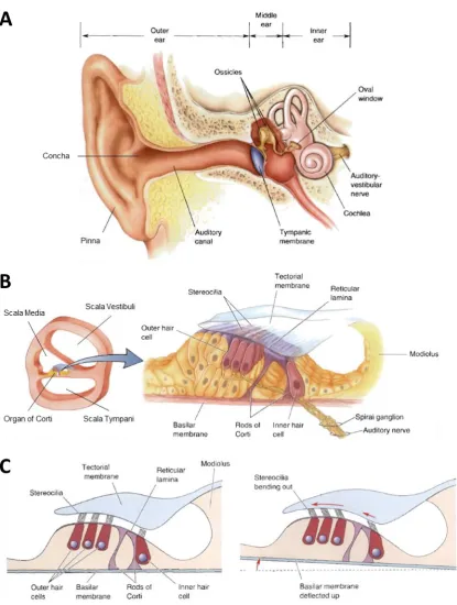
The peripheral auditory system can be broken down into three subsections, specifically the outer-, middle-, and inner-ear (Figure 2.1).

16 The middle-ear is an air-filled cavity, comprising three small bones known as the ossicles, i.e., the malleus, incus, and stapes, that contact another flexible membrane on the cochlea, known as the oval window (Figure 2.1A). As sound waves impinge upon the tympanic membrane, the resulting vibrations are transmitted mechanically through the ossicles to the oval window. The main purpose of the middle-ear is to act like a transformer, matching the impedance of the ear canal to the much higher impedance of the cochlear fluids. This is predominantly achieved by virtue of the scaling down—in terms of area—between the tympanic membrane and the oval window—or more accurately the stapes footplate on the oval window—which increases the pressure at the latter (Pickles, 2008, p. 15).

The inner-ear is made up of a snail-shaped tubular structure embedded in the temporal bone called the cochlea, and its connections to the auditory nerve (Figure 2.1A). If the cochlea were cut cross-sectionally, one would see that the tube is divided into three fluid-filled chambers, i.e., the scala vestibuli, the scala media, and the scala tympani (Figure 2.1B). The scala media and scala tympani are separated by the basilar membrane, upon which sits the organ of Corti, and over which hangs the tectorial membrane. The organ of Corti contains ~20,000 hair cells, so-called as they have hair-like stereocilia extending from their top (Figure 2.1C; Bear et al., 2007, p. 354). Hair cells can be divided into inner and outer hair cells depending on their location with respect to the rods of Corti, and are innervated by auditory nerve fibres with their cell bodies in the spiral ganglion (Bear et al., 2007, p. 354; Pickles, 2008, p. 73).

17 (Bear et al., 2007, p. 354). The cochlea can be thought of as an analogue filter bank, that splits incoming soundwaves into logarithmically-spaced frequency bands.

Figure 2.1: Peripheral Auditory System

18

Central Auditory System

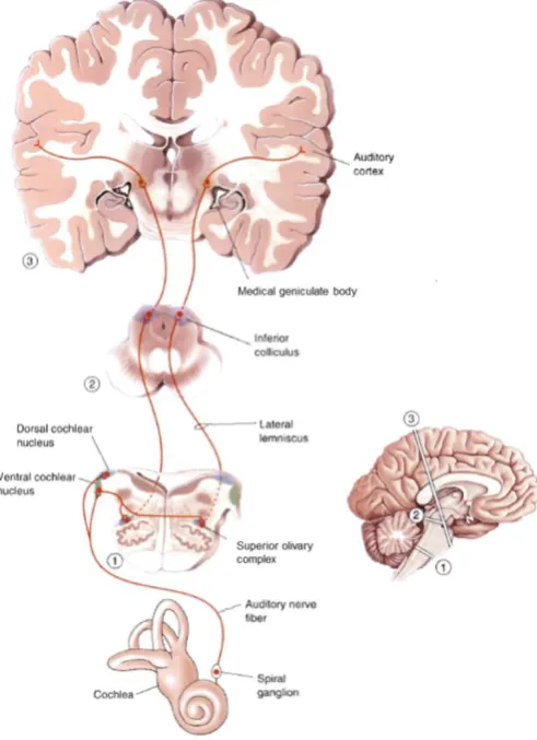
Electrical signals leaving the cochlea travel to the cochlear nucleus via the auditory nerve (Figure 2.2). The cochlear nucleus then projects to higher nuclei through two main streams: the ventral and dorsal streams. Processes in the ventral stream are predominantly concerned with sound localisation, while processes in the dorsal stream are predominantly concerned with sound identification (Pickles, 2008, p. 155). The ventral (sound localisation) stream runs to the superior olivary nuclei on both sides, and up through the lateral lemniscus to the inferior colliculus, while the dorsal (sound identification) stream runs primarily through the lateral lemniscus to the inferior colliculus on the opposite side (Pickles, 2008, p. 170). The inferior colliculus forms the primary site of convergence for these streams, and is a critical stage in the transformation from simple auditory responses to complex auditory objects (Pickles, 2008, p. 183). The inferior colliculus then projects up to the medial geniculate body, which acts as an auditory relay between the inferior colliculus and auditory cortex.

Figure 2.2: Central Auditory System

19

Auditory Cortex

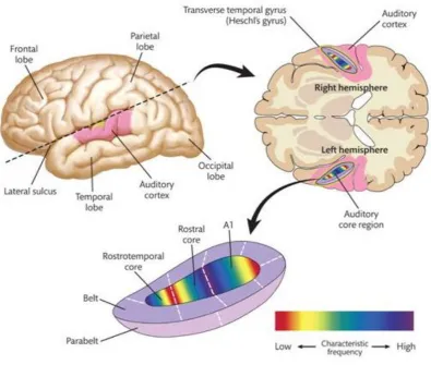
The auditory cortex is located in the superior portion of the temporal lobe (Figure 2.3). It can be subdivided into three areas, i.e., the core, belt, and parabelt, the functions of which tend to show a progressive increase in complexity from inside out. The core is located deep within the lateral sulcus and receives input from the medial geniculate body. Like the cochlea, the core is tonotopically organised (Pickles, 2008, p. 207). The belt is a narrow band of cortex that surrounds the core, that also receives input from the medial geniculate body as well as the core (Pickles, 2008, p. 209). Belt regions are highly interconnected and can also be tonotopically organised. The parabelt receives input from the belt, and is connected to several areas of the frontal, parietal and temporal lobes. These areas tend to be involved in high-level, e.g., speech, processing and are beyond the scope of this thesis.

Figure 2.3: Auditory Cortex

20

Pathophysiology of Human Auditory Processing

Conductive Hearing Loss

Conductive hearing loss refers to hearing loss due to some abnormality in the outer- or middle-ear. In these parts of the hearing system, sound is transferred through movement, e.g., the movement of air along the ear canal or the movement of the tympanic membrane and ossicles, and so the cause of conductive hearing loss tends to be something that impedes this movement in some way, e.g., the ear canal may be blocked, the tympanic membrane damaged, or the ossicles immobilised due to ossification, etc. This type of hearing loss can be well compensated by hearing aids, and in more severe cases surgical interventions, e.g., by replacing the stapes with a prosthesis (Pickles, 2008, p. 309).

Sensorineural Hearing Loss

Sensorineural hearing loss refers to hearing loss due to some problem arising in the cochlea or auditory nerve. While this can be caused by a benign tumour around the sheath of the auditory nerve known as an acoustic neuroma, it is most commonly an issue with the hair cells of the cochlea. These issues can be caused by acoustic trauma, drugs, infections, or may be congenital or due to old age (Pickles, 2008, p. 309). Unfortunately, hearing aids tend to be of limited use for this type of hearing loss, although in more severe cases cochlear implants—electronic prostheses that aim to replicate the mechanical-to-electrical transduction of the cochlea—can provide a limited sensation of hearing to those who otherwise would have none.

Hidden Hearing Loss

21 While this type of hearing loss can remain “hidden” with PTA, it can be revealed using appropriate high-level measures, such as those involving dichotic listening, speech-in-noise, etc.

Electrophysiology of Low-Level Human Auditory

Processing

Electroencephalography

Once the mechanical-to-electrical transduction has taken place in the cochlea, auditory processing becomes electrical—or more specifically, electrochemical—in nature. Signals propagate along the auditory pathway in the form of action potentials—all-or-nothing electrochemical events that depolarise sections of nerve fibres, and neurons, provided that sufficient membrane potentials have been met. These electrical signals can be recorded using electrodes placed on the surface of the scalp using a technique referred to as EEG and can provide objective measures of auditory processing.

The connections between neurons are known as synapses, and it is typically the electrical fields generated by synchronous postsynaptic activity from many neurons that is what is recorded with EEG. As EEG electrodes are placed on the surface of the scalp, these electrical fields need to pass through several anatomical layers, e.g., cerebrospinal fluid, bone, and skin, before reaching the electrode surface. This leads to an attenuation of the signal, particularly in-contrast to other larger electrophysiological signals such as those of the electrooculogram (EOG), e.g., as a result of blinking or eye movement, or electromyogram (EMG), e.g., as a result of muscle movement, which are often also recorded along with the EEG. It can also lead to spatial smearing at the scalp—particularly as a result of passing through the skull (Srinivasan et al., 1996)—meaning that the activity recorded at a single electrode can comprise a mixture of underlying sources (Makeig et al., 1996).

22

Electrophysiological Measures of Low-Level Human Auditory Processing

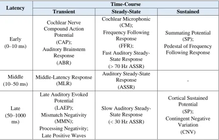
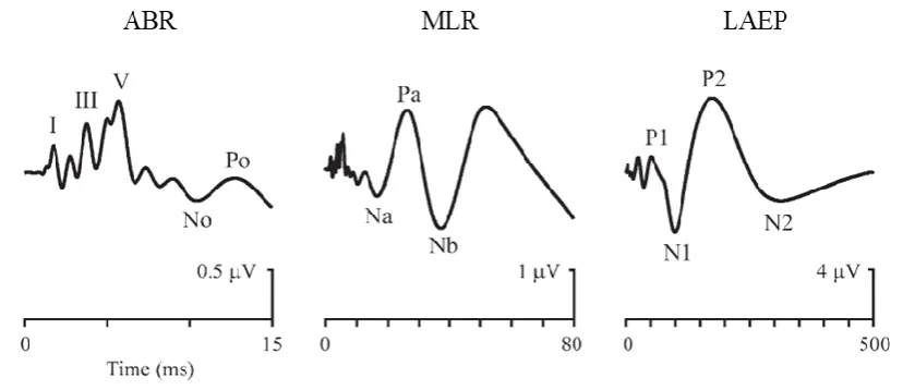
There are numerous measures of low-level human auditory processing that can be recovered with EEG. These can be categorised by latency and time-course (Table 2.1). The measures that are of most relevance to this work are the early, middle, and late transient responses (Picton, 2010, p. 5), specifically the auditory brainstem response (ABR), the middle-latency response (MLR), and the late auditory evoked potential (LAEP), which together comprise the multiple-latency AEP. The reason that these responses are so relevant to the current work is that they can be considered as special cases of the TRF (see Chapter 3 for details). Briefly, the AEP is the auditory system response to (quasi-)discrete stimuli while the TRF represents the auditory system response to any stimuli—including (quasi-)discrete stimuli.

Table 2.1: Low-Level Auditory Responses

Latency Time-Course

Transient Steady-State Sustained

Early (0–10 ms) Cochlear Nerve Compound Action Potential (CAP); Auditory Brainstem Response (ABR) Cochlear Microphonic (CM); Frequency Following Response (FFR); Fast Auditory

Steady-State Response (> 70 Hz ASSR)

Summating Potential (SP);

Pedestal of Frequency Following Response Middle (10–50 ms) Middle-Latency Response (MLR) Auditory Steady-State Response (ASSR) - Late (50–1000 ms)

Late Auditory Evoked Potential (LAEP); Mismatch Negativity

(MMN); Processing Negativity;

Late Positive Waves

Slow Auditory Steady-State Response (< 30 Hz ASSR)

Cortical Sustained Potential (SP); Contingent Negative Variation (CNV)

Auditory Evoked Potential

23 evaluated (Burkard et al., 2007, p. 230). While it can be helpful to think of each wave as representing a distinct stage of neural processing along the auditory pathway, most waves— apart from wave I which is generated solely by the auditory nerve—are generated by multiple neural sources.

The MLR refers to the transient response recorded from the upper brainstem and thalamic nuclei, i.e., the late central auditory system and auditory cortex, between 10–50 ms after the onset of a brief sound (Figure 2.4). It comprises a series of 5 waves—2 positive and 3 negative—i.e., No-Po-Na-Pa-Nb, following the convention of Goldstein and Rodman (1967). N and P denote the polarity of the waves when recorded at the vertex. The shape and amplitude of these waves are sensitive to stimulus, subject, and recording factors.

The LAEP refers to the transient response recorded from the auditory cortex, between 50–1000 ms after the onset of a brief sound. It comprises a series of 4 waves—2 positive and 2 negative—i.e., P1-N1-P2-N2, following the convention of Williams et al., (1962). The shape and amplitude of these waves are also sensitive to stimulus, subject, and recording factors.

Figure 2.4: ABR, MLR, and LAEP

Example ABR, MLR, and LAEP with labelled waves. Please note the different time and amplitude scales used. Adapted from Picton (2013).

Recovering Auditory Evoked Potentials

24 noting, however, that this increase in SNR is proportional to the square root of the number of averages (Hall, 1992, p. 82), and so comes with diminishing returns. The exquisite temporal resolution afforded by TDA has produced the canonical ABRs, MLRs, and LAEPs that have come to be so heavily studied. As such, TDA has been instrumental in advancing our knowledge of the human auditory system.

One shortcoming of the TDA approach, however, is that one is typically restricted to using (quasi-)discrete stimuli. Another shortcoming is that data collection can be quite slow as the maximum rate at which stimuli can be presented is limited. This is because a succeeding stimulus typically cannot be presented until the response to the preceding stimulus has ended, as otherwise a confusing overlap of responses would occur. Traditionally, this has meant that separate sets of specialised stimuli and resulting neural data are required to assess each auditory latency of interest, i.e., it has not been possible to recover multiple-latency responses using just one set of stimuli and resulting EEG.

25 Figure 2.5: Time-Domain Averaging

26

Chapter 3.

Temporal Response Function

Estimation

In this chapter, the TRF estimation approach is introduced. This is followed by a description of its theoretical/mathematical basis, including definitions of relevant terminology, equations, and procedures. Some nomenclature associated with different types of stimulus representations are then defined, followed by a discussion on how to interpret the resulting TRFs. Finally, the relationship between the TRF and AEP is outlined.

Introduction

27 complexity and decrease in interpretability has led to linear modelling approaches being favoured.

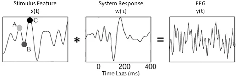
One explicit use of this linear modelling approach has been the fitting of TRFs to describe how EEG is affected by variations in visual (Gonçalves et al., 2014) or—as in this case—auditory stimuli (Lalor et al., 2009). With TRF estimation, the assumption is that the instantaneous output EEG at channel 𝑛 of 𝑁, 𝑦(𝑡, 𝑛), sampled at times 𝑡 = 1 … 𝑇, comprises the linear convolution of an input stimulus feature, 𝑥(𝑡 − 𝜏), with an unknown system response, 𝑤(𝜏, 𝑛), i.e., the TRF, plus noise (Figure 3.1):

𝑦(𝑡, 𝑛) = ∑ 𝑤(𝜏, 𝑛)𝑥(𝑡 − 𝜏)

𝜏

+ 𝜀(𝑡, 𝑛)

where 𝜏 represents the range of time-lags over which the TRF is estimated, and 𝜀(𝑡) represents the residual EEG not explained by the model (Crosse et al., 2016). The range of time-lags used to derive a TRF is typically similar to that used to recover an AEP, although the interpretation of their timing is somewhat different. For example, the value of an AEP at 100 ms describes the average response in the EEG 100 ms after stimulus onset, whereas the value of a TRF at 100 ms describes how a change in the stimulus feature will affect the EEG 100 ms later (Lalor et al., 2009).

Figure 3.1: TRF Estimation

With TRF estimation, the assumption is that the output EEG, 𝒚(𝒕), consists of the convolution of a particular input stimulus feature, 𝒙(𝒕), with an unknown system response, i.e., the TRF,

28

Forward Models

TRFs that describe the mapping from the stimulus feature to the EEG are known as forward models. Forward models are derived by minimising the mean-squared error (MSE) between the predicted EEG, 𝑦̂(𝑡, 𝑛), and measured EEG, 𝑦(𝑡, 𝑛):

min 𝜀(𝑡, 𝑛) = ∑[𝑦̂(𝑡, 𝑛) − 𝑦(𝑡, 𝑛)]2

𝑡

In practice this is done using linear regression:

𝑤 = (𝑋𝑇𝑋)−1𝑋𝑇𝑦

where 𝑦 is a matrix of EEG data with channels arranged column-wise, 𝑋 is the design matrix or lagged time series of the stimulus feature 𝑥(𝑡):

𝑥(1 − 𝜏𝑚𝑖𝑛) 𝑥(−𝜏𝑚𝑖𝑛) ⋯ 𝑥(1) 0 ⋯ 0

⋮ ⋮ ⋯ ⋮ 𝑥(1) ⋯ ⋮

⋮ ⋮ ⋯ ⋮ ⋮ ⋯ 0

⋮ ⋮ ⋯ ⋮ ⋮ ⋯ 𝑥(1)

𝑋 = 𝑥(𝑇) ⋮ ⋯ ⋮ ⋮ ⋯ ⋮

0 𝑥(𝑇) ⋯ ⋮ ⋮ ⋯ ⋮

⋮ 0 ⋯ ⋮ ⋮ ⋯ ⋮

⋮ ⋮ ⋯ ⋮ ⋮ ⋯ ⋮

0 0 ⋯ 𝑥(𝑇) 𝑥(𝑇 − 1) ⋯ 𝑥(𝑇 − 𝜏𝑚𝑎𝑥) where 𝜏𝑚𝑖𝑛 and 𝜏𝑚𝑎𝑥 are the minimum and maximum time lags (in samples) respectively, 𝑋𝑇𝑋 is the autocovariance matrix—which can be problematic to invert—and 𝑋𝑇_{𝑦 is the} cross-covariance matrix (Crosse et al., 2016). In 𝑋, each time lag is arranged column-wise and non-zero lags are padded with non-zeros to ensure causality (Mesgarani et al., 2009). The window or window of support over which the TRF is calculated is defined as 𝜏𝑤𝑖𝑛𝑑𝑜𝑤 = 𝜏𝑚𝑎𝑥− 𝜏𝑚𝑖𝑛, and so the dimensions of 𝑋 are 𝑇 × 𝜏_{𝑤𝑖𝑛𝑑𝑜𝑤}, although a column of ones is also concatenated to the left of 𝑋 to include the y-intercept in the regression model (Crosse et al., 2016). 𝑦 has dimensions 𝑇 × 𝑁 and the resulting TRF, 𝑤, has dimensions 𝜏_{𝑤𝑖𝑛𝑑𝑜𝑤}× 𝑁, where each column represents the mapping between the stimulus feature and EEG at a different channel (Crosse et al., 2016).

Backward Models

stimulus-29 response mappings are derived for each EEG channel, whereas with backward modelling, all of the available data is exploited simultaneously when deriving reverse stimulus-response mappings (Crosse et al., 2016). This makes backward models more sensitive to small differences between EEG channels that are highly correlated with each other—as is often the case with EEG (Crosse et al., 2016)—although this does come at the cost of direct neurophysiological interpretability (Haufe et al., 2014).

Like forward models, backward models are derived by minimising the MSE between the reconstructed stimulus feature, 𝑥̂(𝑡), and actual stimulus feature, 𝑥(𝑡):

min 𝜀(𝑡) = ∑[𝑥̂(𝑡) − 𝑥(𝑡)]2

𝑡

Again, in practice, this is done using linear regression:

𝑔 = (𝑌𝑇_𝑌)−1_𝑌𝑇_𝑥

where 𝑥 is a column-wise vector or matrix containing the stimulus feature—depending on whether it is a univariate or multivariate feature, e.g., an envelope or spectrogram—and 𝑌 is the lagged time series of the EEG matrix, 𝑦. For simplicity, for a single channel system:

𝑦(1 − 𝜏𝑚𝑖𝑛, 1) 𝑦(−𝜏𝑚𝑖𝑛, 1) ⋯ 𝑦(1,1) 0 ⋯ 0

⋮ ⋮ ⋯ ⋮ 𝑦(1,1) ⋯ ⋮

⋮ ⋮ ⋯ ⋮ ⋮ ⋯ 0

⋮ ⋮ ⋯ ⋮ ⋮ ⋯ 𝑦(1,1)

𝑌 = 𝑦(𝑇, 1) ⋮ ⋯ ⋮ ⋮ ⋯ ⋮

0 𝑦(𝑇, 1) ⋯ ⋮ ⋮ ⋯ ⋮

⋮ 0 ⋯ ⋮ ⋮ ⋯ ⋮

⋮ ⋮ ⋯ ⋮ ⋮ ⋯ ⋮

0 0 ⋯ 𝑦(𝑇, 1) 𝑦(𝑇 − 1,1) ⋯ 𝑦(𝑇 − 𝜏𝑚𝑎𝑥, 1) The range of time-lags, 𝜏, used here would typically be similar to that used in forward modelling except in the reverse direction, as it is effectively mapping backwards in time (Crosse et al., 2016). So instead of the lags ranging from -100 to 400 ms for example, they would range from -400 to 100 ms. The dimensions of 𝑌 for a single channel system are

𝑇 × 𝜏𝑤𝑖𝑛𝑑𝑜𝑤, although a column of ones is also concatenated to the left of 𝑌 to include the

30

Regularisation

Two issues that can arise when deriving TRFs involve the inversion of ill-conditioned matrices, and overfitting. Matrix inversion is prone to numerical instability when solved with finite precision, and so small changes in the autocovariance matrix, 𝑋𝑇𝑋, can cause large changes in the TRF if the former is ill-conditioned (Crosse et al., 2016). Overfitting occurs when a TRF has become optimally fit for a particular dataset but does not generalise well to unseen data. This is often because the TRF has also been fit to the “noise” in the data it has been trained on, which is unlikely to be present in any other (Crosse et al., 2016). Both issues can be improved using a method known as regularisation, i.e., the introduction of a bias or “smoothing” term to reduce the variance in the TRF.

In practice, regularisation can be carried out by weighting the diagonal of 𝑋𝑇𝑋 before inversion—a method known as ridge regression:

𝑤 = (𝑋𝑇𝑋 + 𝜆𝐼)−1𝑋𝑇𝑦

where 𝜆 is the bias term (regularisation parameter) and 𝐼 is the identity matrix. This form of regularisation enforces a smoothness constraint on the TRF by penalising TRF values as a function of their distance from zero (Crosse et al., 2016). Another option is to quadratically penalise the difference between each two neighbouring terms of the TRF, a method known as Tikhonov regularisation (Tikhonov, 1963):

𝑤 = (𝑋𝑇𝑋 + 𝜆𝑀)−1𝑋𝑇

where:

1 −1

−1 2 −1

𝑀 = −1 2 −1

⋱ ⋱ ⋱

−1 2 −1

−1 1

31

Model Fitting Procedure

The first step when deriving TRFs is to fit a separate model for each of M trials. One trial is then typically chosen to be left-out, i.e., to be used as the validation/test set, with the remaining M-1 trials to be used as the training set. An average model is then attained by averaging over the single-trial models in the training set, before being convolved with the stimulus feature associated with the validation/test set to predict its EEG response. Model performance is then assessed by quantifying how accurately the predicted EEG response matches the recorded EEG response in the validation/test set. This measure is often attained using Pearson’s correlation coefficient and is referred to as prediction accuracy. This entire process—which is referred to as cross-validation—is then repeated M-1 times such that each trial is left-out of the training set once. The overall model performance can then finally be determined by averaging over the individual model performances for each trial (Crosse et al., 2016).

This procedure can also be carried out in the backward direction, where instead of trying to predict the EEG response of the left-out trial, one is trying to reconstruct the stimulus feature used to elicit its EEG response (Crosse et al., 2016). In this case, model performance can be assessed by quantifying how accurately the reconstructed stimulus feature matches the presented stimulus feature associated with the validation/test set. This measure is again often attained using Pearson’s correlation coefficient and is referred to as reconstruction accuracy. Because the models are fit using regularisation, it is also necessary to determine the optimal lambda value. This is done by repeating the cross-validation procedure for each of several lambda values and then choosing the value that results in the best prediction/reconstruction accuracy.

Stimulus Representation

32 from multiple latencies simultaneously, i.e., using just one set of stimuli and resulting EEG, and does so while permitting a wider variety of stimuli to be used.

Given that the modelling approach and EEG are typically fixed, the choice of stimulus feature and the way in which it is represented—collectively referred to as the stimulus representation—plays an important role in determining the resulting model. For example, depending on whether one uses a global measure of amplitude change like the envelope, or a multivariate binary representation of phoneme activity, such as the phoneme representation introduced by Di Liberto et al. (2015a), one can interrogate very different aspects of auditory processing. How these stimulus representations are generated, and what they can be used for will be discussed in more detail throughout the thesis. First, however, it would be useful to define a nomenclature with which to describe them.

Feature

‘Feature’ refers to some property of the original stimulus that is encapsulated by the stimulus representation. Classically the envelope has been used (Lalor and Foxe, 2010) but other features such as the raw audio signal (Maddox and Lee, 2018), phonemes, phonetic features (Di Liberto et al., 2015), and semantic dissimilarity (Broderick et al., 2018) have also proven useful. The choice of feature is dependent on the attribute and/or result of interest.

Form

‘Form’ refers to the way in which the stimulus representation is expressed. For example, stimulus representations are typically expressed in their voltage form, i.e., the form in which they are stored in the audio file. However, as electrophysiological responses tend to vary in proportion to the log of the stimulus amplitude, for example (Aiken and Picton, 2008), they could also be represented in their in their log or “sound pressure level” (SPL) form (as in Chapter 6).

Compensation

33 depending on the goal, e.g., the application of a gammachirp filter bank would obviously be inappropriate if trying to study the cochlear-neural time-delay.

Calculation

‘Calculation’ refers to the calculation of some higher-order feature from the original stimulus feature. For example, this could be the positive or negative half-wave rectified audio signal (Maddox and Lee, 2018), the full-wave rectified audio signal, the positive half-wave rectified first derivative (onset) of the envelope (Hertrich et al., 2012; Fiedler et al., 2016; as in Chapter 6), the negative half-wave rectified first derivative (offset) of the envelope, or the full-wave rectified first derivative of the envelope.

Binning

‘Binning’ refers to the binning of the stimulus representation based on chosen attributes. The stimulus representation could be frequency-binned (FB), i.e., a spectrogram, amplitude-binned (AB; as in Chapter 6), or frequency- and amplitude-binned (FAB).

Value

‘Value’ refers to the value given to the binned features. For example, these could be their original values, or perhaps they may be categorical such as phonetic features and so be represented as binary, or in the case of semantic dissimilarity, the value of the feature corresponds to the semantic dissimilarity at that point.

The specific combination of these parameters can be used to describe the stimulus representation. For example, a raw audio signal stored in a WAV file or similar, could be referred to simply as a voltage signal, while an audio signal that has been passed through a gammachirp filter bank, had its envelope extracted, transformed to SPL, and amplitude-binned, could be referred to as an AB gammachirp SPL envelope. There are certain situations where parameters are implicit, but for others perhaps this format could be useful.

Interpretation

34 representation that is exemplary of that hypothesis, and then evaluating its fit using the resulting prediction or reconstruction accuracies. If the chosen feature is indeed represented in the brain in the manner hypothesised, it should result in high prediction or reconstruction accuracies. What is defined as “high” in this instance is relative, as the actual values tend to be quite low. This is because the ratio of EEG associated with the stimulus representation to EEG not associated with the stimulus representation also tends to be quite low, and so, prediction and reconstruction accuracies need to be interpreted in this light. Analysis of the model parameters themselves can also provide some insight. For example, one can examine and compare the TRF values at different channels and time-lags to determine which cortical regions may be contributing to the response, and when. These approaches are used extensively throughout the thesis.

Relationship to AEP

35

Chapter 4.

Indexing the Human Auditory

Processing Hierarchy: Considerations of

Stimulus Type, Stimulus Representation, and

Computational Efficiency

In this chapter, two approaches for indexing low-level processing along the auditory pathway are introduced over two experiments: Experiment 1 and 2. Experiment 1 is an initial exploratory attempt to derive multiple-latency responses to high-rate click trains. Experiment 2 is a more thorough attempt to derive multiple-latency responses to AM BBN, while introducing a novel efficient TRF estimation approach. A manuscript on Experiment 2 is in preparation at the time of writing for submission to the Journal of the Acoustical Society of America.

Experiment 1

Introduction

36 i.e., it has not been possible to recover multiple-latency responses using just one set of stimuli and resulting EEG. Facilitating the efficient recovery of these canonical responses could have wide ranging benefits for both research and clinical applications where these responses remain instrumental.

As also mentioned in Chapter 2, several methods have permitted faster presentation rates to be used by attempting to account for the overlapping responses. These include MLS deconvolution (Eysholdt and Schreiner, 1982), the ADJAR technique (Woldorff, 1993), CLAD (Delgado and Ozdamar, 2004), QSD (Jewett et al., 2004), RSA (Valderrama et al., 2012), MSAD (Wang et al., 2013), and LS deconvolution (Bardy et al., 2014). While these methods have enabled recovery from overlapping responses, the presentation rate limit has remained problematic. Other methods focused on the use of slower presentation rates, optimised for the recording of dual- or multiple-latency responses (Bidelman, 2015; Kohl and Strauss, 2016) have been more successful, but have also necessarily resulted in certain compromises.

As TRF estimation has been shown to be effective in the derivation of responses to continuous stimuli (Lalor et al., 2009; Lalor and Foxe, 2010), we were curious as to whether it could be used to improve upon previous efforts to permit faster discrete presentation rates. To the author’s knowledge, this had not been attempted before, i.e., it was not known at the time of this experiment’s inception that a similar approach had been proposed by Bardy et al., (2014). Hence, in this experiment we aim to investigate the utility of TRF estimation in the derivation of canonical multiple-latency responses to high-rate click trains. The effectiveness of this approach will be determined through comparisons with canonical AEPs to suitable-rate click trains, derived using TRF estimation.

Materials and Methods

Subjects

37

Stimuli

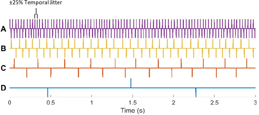
Alternating 100 µs click trains with uniformly distributed ±25% temporal jitter, were presented at rates of 58.4, 21.9, 7.3, and 1.0 Hz (Figure 4.1). These specific rates were chosen because they are suitable—in terms of having sufficiently long SOAs—for evoking canonical ABRs— with some degradation of the earlier waves—ABRs—with little degradation of the earlier waves—MLRs, and LAEPs, respectively.

Figure 4.1: Example Segments of the Stimuli Used in This Experiment

A–D – Alternating 100 µs click trains with uniformly distributed ±25% temporal jitter, presented at 58.4, 21.9, 7.3, and 1.0 Hz, respectively.

Experimental Procedure

38 headphones (ISO 389-6:2007). The click trains were presented using Sennheiser HD 650 headphones, via Presentation software from Neurobehavioral Systems (http://www.neurobs.com). The stimulus presentation order, i.e., for each 60 s long stimulus, was pseudorandomised to minimise any potential order effects.

EEG Acquisition

34 channels of EEG data were recorded at 16384 Hz (analog -3 dB point of 3276.8 Hz), using a BioSemi ActiveTwo system (http://www.biosemi.com). 32 cephalic electrodes were positioned according to the standard 10-20 system, with another 2 electrodes located over the left and right mastoids. Triggers indicating the start of each 60 s trial were presented using Neurobehavioral Systems Presentation software for synchronous recording along with the EEG.

EEG Preprocessing

The EEG data were first resampled to 128 Hz using the decimate function in MATLAB (http://www.mathworks.com). The decimate function incorporates an 8th _{order low-pass} Chebyshev Type I infinite impulse response (IIR) anti-aliasing filter. This filter was implemented using the filtfilt function, ensuring zero phase distortion and in effect doubling the order of the filter. A 1st _{order high-pass Butterworth filter was then applied with a cutoff} frequency of 1 Hz, also using the filtfilt function. Bad channels were determined as those whose variance was either less than half or greater than twice that of the surrounding 2–4 channels, depending on location. These were then replaced through spherical spline interpolation using EEGLAB (Delorme and Makeig, 2004). Finally, the data were rereferenced to the average of the mastoids, separated into trials based on the triggers provided, and z-scored.

Temporal Response Function Estimation

39

Results

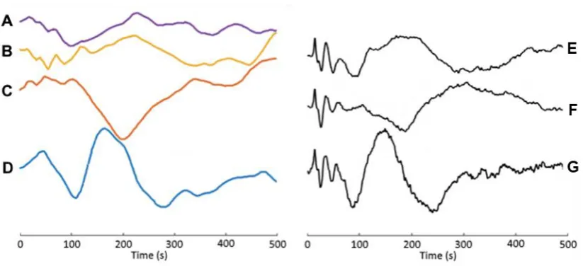
First, grand average click train LAEPs were derived in response to each of the four click train stimuli, and the resulting waveforms plotted—stacked on top of one another—on the left-hand side of Figure 4.2. It is clear from these plots that the morphologies (shapes) of the 58.4, 21.9, and 7.3 Hz click train LAEPs are quite different from that of the canonical 1.0 Hz click train LAEP. This—albeit qualitative—comparison indicates that it is not possible to derive canonical multiple-latency responses to high-rate click trains using TRF estimation, and that any efforts to derive MLRs or ABRs would be moot.

These results concur with previous efforts to derive multiple-latency responses using high-rate discrete stimuli. Indeed these results effectively mirror those of high-rate chirp train LAEPs derived using CLAD (Holt and Özdamar, 2016; right-hand side of Figure 4.2). The high degree of similarity between these two sets of responses, suggests that this is due to some fundamental feature of the auditory system rather than being a technical limitation inherent to any one approach.

Figure 4.2: Grand Average Click Train vs. Grand Average Chirp Train LAEPs

A–D – Grand average LAEPs derived to the 58.4, 21.9, 7.3, and 1.0 Hz click trains used in this experiment, respectively. E–G – Grand average LAEPs derived by Holt and Özdamar (2016) to 20.0, 7.0, and 1.0 Hz chirp trains, respectively.

Discussion

40 LAEP. This is likely due to response adaptation at the higher rates, as has been seen with other similar approaches, e.g., CLAD (Holt and Özdamar, 2016). Adaptation in this context refers to changes in response amplitude as a function of SOA. This manifests as changes in response morphology because LAEP waves tend to comprise multiple components and these components tend to be differently affected by SOA (Lü et al., 1992; Sams et al., 1993). Therefore, it is highly unlikely that any approach employing high-rate discrete stimuli would ever be able to derive canonical LAEPs—and thus canonical multiple-latency responses—as the morphology of these responses are fundamentally dependent on the SOAs of the stimuli used to elicit them.

While it may not be possible to derive canonical LAEPs using high-rate discrete stimuli, it is possible to recover LAEPs that display the effects of adaptation. Such responses could be useful in the study of adaptive mechanisms (Burkard et al., 1990; Lasky, 1997) and in the diagnosis of certain pathologies (Tanaka et al., 1996; Jiang et al., 2000). One approach that could be interesting to try in this context, would be to separate the discrete stimuli trains into multiple bins, based on SOA, i.e., as a multivariate stimulus representation. This is similar in principle to how Di Liberto et al. (2015) represented different phonetic features, and could facilitate the study of adaptation at different SOAs.

41

Experiment 2

Introduction

In Experiment 1, we investigated the utility of TRF estimation in the derivation of canonical multiple-latency responses to high-rate click trains and determined that we should focus our efforts on other approaches. These for example could include the use of TRF estimation and continuous stimuli. As mentioned in Chapter 3, this approach has been used successfully in the past, e.g., Lalor et al. (2009) showed that using TRF estimation, it is possible to derive LAEPs to AMTs and AM BBN, Lalor and Foxe (2010) showed that it is possible to derive LAEPs to continuous natural speech, and recently, Maddox and Lee (2018) modified this approach and showed that it is possible to derive responses to continuous natural speech, from the entire auditory pathway simultaneously.

Here we aim to build upon the work of Lalor et al. (2009), Lalor and Foxe (2010), and Maddox and Lee (2018), by focusing on the derivation of multiple-latency responses to AM BBN. Specifically, we aim to demonstrate that the specificity of these responses and the efficiency of their derivation can be further improved using different stimulus representations and modelling approaches respectively. We also propose to further the investigation of their neural underpinnings through comparisons with their canonical counterparts, elicited using level-specific (LS) chirp trains (Elberling and Don, 2010; Elberling et al., 2012).

Materials and Methods

Subjects

13 subjects aged 23–35 years participated in this study; 5 were male. All subjects had self-reported normal hearing. The protocol for this study was approved by the Ethics Committee of the Health Sciences Faculty at Trinity College Dublin, Ireland, and all subjects gave written informed consent.

Stimuli

42 The carrier signal for the AM BBN stimulus (Figure 4.3A) was uniform BBN with energy limited to a bandwidth of 0–24000 Hz (Figure 6.1C). Its modulating signal had a log-uniform amplitude distribution and a bottom-heavy (right-skewed) frequency (modulation rate) distribution (Figure 6.1E and G)—so chosen as it has been shown that auditory cortical areas tend to be most sensitive to AM stimuli presented at lower modulation rates (Liégeois-Chauvel et al., 2004). The modulating signal was created by first generating a discrete “template” signal, with impulse amplitudes randomly drawn from a beta distribution, i.e., 𝐵(0.65,0.65), and impulse SOAs uniformly randomly set to between 0.125 s and 0.0313 s, resulting in instantaneous presentation rates of between 8 and 32 Hz. Another signal was then created by interpolating between the different impulses in the template signal, resulting in a continuous signal with a slightly more Gaussian amplitude distribution than the template—and so uniform overall given that the template signal had a slightly “U-shaped” beta amplitude distribution— and a more bottom-heavy modulation rate distribution—given that the amplitude at each impulse now only contributed to at most half of a full-cycle in the continuous signal, although typically less than that as the impulse amplitudes did not always alternate consecutively, thus, at least halving the instantaneous presentation rates to between 4 and 16 Hz. Finally, the continuous modulating signal—which was assumed to be in its SPL form—was transformed into its voltage form using:

𝑥_{𝑣𝑜𝑙𝑡𝑎𝑔𝑒} = 10((80×𝑥𝑆𝑃𝐿)/20)

where 𝑥𝑣𝑜𝑙𝑡𝑎𝑔𝑒 is the modulating signal in its voltage form, 𝑥𝑆𝑃𝐿 is the modulating signal in its SPL form, and 80 refers to the maximum presentation level in dB SPL. This was done so that when the modulating signal was applied across the transducer, it would be transformed back into its SPL form with a uniform amplitude distribution as intended.

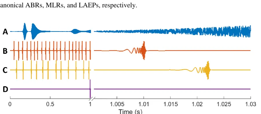
43 also take the influence of stimulus level on response latency into account (Elberling et al., 2012).

Here, alternating 60 dB nHL LS-Chirp trains with uniformly distributed ±25% jitter were presented at rates of 20.1, 12.3, and 1.0 Hz (Figure 4.3B–D). These specific rates were chosen because they are suitable—in terms of having sufficiently long SOAs—for evoking canonical ABRs, MLRs, and LAEPs, respectively.

Figure 4.3: Example Segments of the Stimuli used in This Experiment.

A – The AM BBN stimulus. B–D – Alternating 60 dB nHL LS-Chirp trains, with uniformly distributed +/-25% temporal jitter, presented at 20.1, 12.3, and 1.0 Hz, respectively. Please note the variable timescale on the x-axis which is there to provide both a sense of their overall time-course (left, 0 to 1 s) and their fine temporal detail (right, 1 to 1.03 s).

Experimental Procedure

44 Etymotic Research ER-2 earphones, via VLC Media Player from VideoLan (http://www.videolan.org). The stimulus presentation order, i.e., for each 60 s long stimulus, was pseudorandomised to minimise any potential order effects. Compensation for the 1 ms sound tube delay introduced by the ER-2 earphones was applied post-hoc.

EEG Acquisition

40 channels of EEG data were recorded at 16384 Hz (analog -3 dB point of 3276.8 Hz), using a BioSemi ActiveTwo system (http://www.biosemi.com). 32 cephalic electrodes were positioned according to the standard 10-20 system. A further eight non-cephalic electrodes were also collected although only two—those over the left and right mastoids—were used in the analysis. Triggers indicating the start of each 60 s trial were encoded in a separate channel in the stimulus WAV file as three cycles of a 16 kHz tone burst. These triggers were interpreted by custom hardware before being fed into the acquisition laptop for synchronous recording along with the EEG.

EEG Preprocessing

The EEG data were first resampled to the appropriate rate (see below) using the decimate function in MATLAB (http://www.mathworks.com). The decimate function incorporates an 8th _{order low-pass Chebyshev Type I IIR anti-aliasing filter, implemented using the filtfilt} function. A 1st order high-pass Butterworth filter was then applied with a cutoff frequency of 1 Hz, also using the filtfilt function. 5 Hz wide 1st order notch Butterworth filters were then applied with centre frequencies of 50, 150, 450, and 750 Hz, i.e., the electrical mains frequency, and the first three triplen harmonics, again using the filtfilt function. Bad channels were determined as those whose variance was either less than half or greater than twice that of the surrounding 2–4 channels, depending on location. These were then replaced through spherical spline interpolation using EEGLAB (Delorme and Makeig, 2004). Finally, the data were rereferenced to the average of the mastoids, separated into trials based on the triggers provided, and z-scored.

Temporal Response Function Estimation

45 consideration with these calculations is the so-called window of support, i.e., the range of time-lags over which the TRF is to be estimated. As will become clear below, this range was chosen in different ways to emphasise the different auditory latencies. In all cases, baseline correction was performed on each subject’s average TRF by subtracting the mean of certain pre-stimulus values, i.e., ABR: -5 to 0 ms; MLR: -10 to 0 ms; LAEP: -20 to 0 ms, before being combined to form the grand average response.

AM BBN Stimulus Representations

As mentioned, an important consideration when employing TRF estimation is the choice of stimulus feature. As the defining characteristic of AM BBN is its amplitude envelope, it is the obvious feature of choice. It is worth noting that while envelopes used in previous studies have often been too slow for studying the fast dynamics of subcortical nuclei, envelopes extracted from higher sampling-rate representations of the audio signal can contain the requisite high-rate fluctuations. Here, the envelope representation was genehigh-rated by first resampling the original audio signal down to 24576 Hz using the decimate function in MATLAB, then taking the absolute value of its Hilbert transform, before finally resampling it down to 8192 Hz.

One issue with this representation, however, is that given the strong relationship between stimulus frequency and ABR latency—due to the tonotopic nature of the cochlea—an ABR derived using a broadband envelope is likely to be temporally smeared. This could perhaps be ameliorated using an approach akin to the stacked ABR, where a number of different narrowband ABRs are first recovered, then realigned in time and summed (Don et al., 1997). In this case, such responses could be derived separately for each frequency component or perhaps simultaneously using a FB (spectrogram) representation (Ding and Simon, 2012; Di Liberto et al., 2015). However, given the temporal cost of the former and the computational cost of the latter—particularly given the high sampling rates used here—neither of these approaches were preferred.

46 12288 Hz, then extracting the envelopes from each band and averaging them together, before finally resampling it down to 8192 Hz.

Modelling Approaches

Maddox and Lee (2018) were the first to show that it is possible to derive responses to continuous natural speech, from the entire auditory pathway simultaneously. However, the high sampling rates that are necessary for deriving the short-latency (ABR) parts of these responses make this a computationally- and memory-intensive analysis—although ameliorated in their case using a novel Fourier-based approach. This is particularly problematic as the stimulus autocovariance matrix used to derive the TRF grows quadratically with sampling rate. However, the high sampling rates that are necessary for deriving the short-latency parts of these responses are higher than are necessary for deriving the middle- and long-latency (MLR and LAEP) parts of these responses. Therefore, reducing the sampling rates to the minimum necessary when deriving each latency, should help to minimise