A Multigrid Block Krylov Subspace Spectral Method for Variable-Coeﬃcient Elliptic PDE

(1)

A Multigrid Block Krylov Subspace Spectral

Method for Variable-Coeﬃcient Elliptic PDE

James V. Lambers

∗

Abstract—Krylov subspace spectral (KSS) methods have been demonstrated to be effective tools for solv-ing time-dependent variable-coefficient PDE. They employ techniques developed by Golub and Meurant for computing elements of functions of matrices to approximate each Fourier coefficient of the solution using a Gaussian quadrature rule that is tailored to that coefficient. In this paper, we apply this same ap-proach to time-independent PDE of the form 𝐿𝑢=𝑔, where 𝐿 is an elliptic differential operator. Numer-ical results demonstrate the effectiveness of this proach, in conjunction with residual correction ap-plied on progressively finer grids, for Poisson’s equa-tion and the Helmholtz equaequa-tion.

Keywords: spectral methods, Gaussian quadrature, block Lanczos method, Poisson’s equation, Helmholtz equation

1 Introduction

Let𝐿 be an elliptic second-order diﬀerential operator of the form

𝐿𝑢=−∇ ⋅(𝑝∇𝑢) +𝑞𝑢, (1)

where 𝑝(𝑥, 𝑦)>0 and𝑞(𝑥, 𝑦) are smooth functions. We consider the following boundary value problem on a rect-angle,

𝐿𝑢=𝑔(𝑥, 𝑦), 0< 𝑥, 𝑦 <2𝜋, (2)

with homogeneous Dirichlet boundary conditions, or pe-riodic boundary conditions.

In [16] a class of methods, called Krylov subspace spectral (KSS) methods, was introduced for the purpose of solving parabolic variable-coeﬃcient PDE. These methods are based on techniques developed by Golub and Meurant in [5] for approximating elements of a function of a matrix by Gaussian quadrature in thespectraldomain. In [9, 12], these methods were generalized to the second-order wave equation, for which these methods have exhibited even higher-order accuracy.

∗_Submitted _September _7, _2009. _University _of

South-ern Mississippi, Department of Mathematics, Hattiesburg, MS 39406-0001 USA Tel/Fax: 601-266-5784/5818 Email: [email protected]

It has been shown in these references that KSS methods, by employing different approximations of the solution op-erator for each Fourier coefficient of the solution, achieve higher-order accuracy in time than other Krylov subspace methods (see, for example, [10]) for stiff systems of ODE, and, as shown in [12], they are also quite stable, consid-ering that they are explicit methods. In [13, 14], the accuracy and robustness of KSS methods were enhanced using block Gaussian quadrature. Recent extensions in-clude the time-dependent Schrödinger equation [15] and Maxwell’s equations [18].

It is our belief that by a change of integrand in the in-tegrals used to compute the Fourier coefficients of the solution, the high accuracy achieved for time-dependent problems can be extended to the time-independent case, even for cases in which the operator𝐿is indefinite, as in the Helmholtz equation. In this paper, we will see that by applying block KSS methods in conjunction with resid-ual correction, first on coarser grids and proceeding to finer grids, we do in fact obtain a highly accurate and ef-ficient method for these problems. Section 2 reviews the main properties of KSS methods, including block KSS methods, and explains how they can be applied to ellip-tic problems. Numerical results are presented in Section 3, and conclusions are stated in Section 4.

2 Krylov Subspace Spectral Methods

We ﬁrst review KSS methods, which were ﬁrst developed in [16] for parabolic problems. Let 𝑆 = 𝐿−1 _represent

the exact solution operator of the problem (2), restricted to one space dimension for simplicity, and let⟨⋅,⋅⟩denote the standard inner product of functions deﬁned on [0,2𝜋],

⟨𝑢(𝑥), 𝑣(𝑥)⟩= ∫ 2𝜋

0

𝑢(𝑥)𝑣(𝑥)𝑑𝑥. (3)

(2)

applying the exact solution operator to𝑔(𝑥),

ˆ

𝑢(𝜔) = 〈 ₁

√ 2𝜋𝑒

𝑖𝜔𝑥_{, 𝑆𝑔}₍_𝑥₎ 〉

. (4)

2.1 Elements of Functions of Matrices

In [5] Golub and Meurant describe a method for comput-ing quantities of the form

u𝑇𝑓(𝐴)v, (5)

whereuandvare𝑁-vectors,𝐴 is an𝑁×𝑁 symmetric positive deﬁnite matrix, and𝑓 is a smooth function. Our goal is to apply this method with 𝐴 = 𝐿𝑁 where 𝐿𝑁 is a spectral discretization of 𝐿, 𝑓(𝜆) = 𝜆−1_{, and the}

vectorsuandvare derived from ˆe𝜔andg, where ˆe𝜔is a discretization of √1

2𝜋𝑒

𝑖𝜔𝑥_and_g_{represents the right-hand}

side function𝑔(𝑥), evaluated on an𝑁-point uniform grid.

The basic idea is as follows: since the matrix 𝐴is sym-metric positive deﬁnite, it has real eigenvalues

𝑏=𝜆1≥𝜆2≥ ⋅ ⋅ ⋅ ≥𝜆𝑁 =𝑎 >0, (6)

and corresponding orthogonal eigenvectors q𝑗, 𝑗 = 1, . . . , 𝑁. Therefore, the quantity (5) can be rewritten as

u𝑇𝑓(𝐴)v= 𝑁 ∑

𝑗=1

𝑓(𝜆𝑗)u𝑇q𝑗q𝑇𝑗v. (7)

We let 𝑎=𝜆𝑁 be the smallest eigenvalue, 𝑏=𝜆1 be the

largest eigenvalue, and deﬁne the measure𝛼(𝜆) by

𝛼(𝜆) = ⎧  ⎨

 ⎩

0, if𝜆 < 𝑎

∑𝑁

𝑗=𝑖𝛼𝑗𝛽𝑗, if𝜆𝑖≤𝜆 < 𝜆𝑖−1

∑𝑁

𝑗=1𝛼𝑗𝛽𝑗, if𝑏≤𝜆

, (8)

where 𝛼𝑗 =u𝑇q𝑗 and𝛽𝑗=q𝑇𝑗v.If this measure is posi-tive and increasing, then the quantity (5) can be viewed as a Riemann-Stieltjes integral

u𝑇𝑓(𝐴)v=𝐼[𝑓] = ∫ 𝑏

𝑎

𝑓(𝜆)𝑑𝛼(𝜆). (9)

As discussed in [5], the integral𝐼[𝑓] can be approximated using Gaussian quadrature rules, which yield an approx-imation of the form

𝐼[𝑓] = 𝐾 ∑

𝑗=1

𝑤𝑗𝑓(𝑡𝑗) +𝑅[𝑓], (10)

where the nodes 𝑡𝑗, 𝑗 = 1, . . . , 𝐾, as well as the weights

𝑤𝑗, 𝑗 = 1, . . . , 𝐾, can be obtained using the symmetric Lanczos algorithm ifu=v, and the unsymmetric Lanc-zos algorithm ifu∕=v (see [8]).

2.2 Block Gaussian Quadrature

In the caseu∕=v, there is the possibility that the weights may not be positive, which destabilizes the quadrature rule (see [1] for details). One option to get around this problem is rewriting (5) using decompositions such as

u𝑇𝑓(𝐴)v= 1

𝛿[u

𝑇_𝑓₍_𝐴₎₍_u₊_𝛿_v₎₋_u𝑇_𝑓₍_𝐴₎_u_]_, ₍₁₁₎

where 𝛿 is a small constant. Guidelines for choosing an appropriate value for𝛿can be found in [16, Section 2.2].

If we compute (5) using the formula (11) or the polar decomposition

1

4[(u+v)

𝑇_𝑓₍_𝐴₎₍_u₊_v₎₋₍_v₋_u₎𝑇_𝑓₍_𝐴₎₍_v₋_u_)]_, ₍₁₂₎

then we would have to run the process for approximating an expression of the form (5) with two starting vectors. Instead we consider

[

u v ]𝑇

𝑓(𝐴)[

u v ]

which results in the 2×2 matrix

∫ 𝑏

𝑎

𝑓(𝜆)𝑑𝜇(𝜆) = [

u𝑇𝑓(𝐴)u u𝑇𝑓(𝐴)v v𝑇𝑓(𝐴)u v𝑇𝑓(𝐴)v

]

, (13)

where𝜇(𝜆) is a 2×2 matrix function of 𝜆, each entry of which is a measure of the form𝛼(𝜆) from (8).

In [5] Golub and Meurant show how a block method can be used to generate quadrature formulas. We will describe this process here in more detail. The integral ∫𝑏

𝑎 𝑓(𝜆)𝑑𝜇(𝜆) is now a 2×2 symmetric matrix and the most general𝐾-node quadrature formula is of the form

∫ 𝑏

𝑎

𝑓(𝜆)𝑑𝜇(𝜆) = 𝐾 ∑

𝑗=1

𝑊𝑗𝑓(𝑇𝑗)𝑊𝑗+𝑒𝑟𝑟𝑜𝑟 (14)

with𝑇𝑗and𝑊𝑗being symmetric 2×2 matrices. Equation (14) can be simpliﬁed using

𝑇𝑗=𝑄𝑗Λ𝑗𝑄𝑇𝑗

where 𝑄𝑗 is the eigenvector matrix and Λ𝑗 the 2×2 di-agonal matrix containing the eigenvalues. Hence,

𝐾 ∑

𝑗=1

𝑊𝑗𝑓(𝑇𝑗)𝑊𝑗= 𝐾 ∑

𝑗=1

𝑊𝑗𝑄𝑗𝑓(Λ𝑗)𝑄𝑇𝑗𝑊𝑗

and if we write𝑊𝑗𝑄𝑗𝑓(Λ𝑗)𝑄𝑇𝑗𝑊𝑗 as

(3)

where z𝑘 =𝑊𝑗𝑄𝑗e𝑘 for𝑘= 1,2, we get for the quadra-ture rule

∫ 𝑏

𝑎

𝑓(𝜆)𝑑𝜇(𝜆) =

2𝐾 ∑

𝑗=1

𝑓(𝜇𝑗)v𝑗v𝑇𝑗 +𝑒𝑟𝑟𝑜𝑟,

where 𝜇𝑗 is a scalar and v𝑗 is a vector with two compo-nents.

We now describe how to obtain the scalar nodes𝜇𝑗 and the associated vectors v𝑗. In [5] it is shown that there exist orthogonal matrix polynomials such that

𝜆𝑝𝑗−1(𝜆) =𝑝𝑗(𝜆)𝐵𝑗+𝑝𝑗−1(𝜆)𝑀𝑗+𝑝𝑗−2(𝜆)𝐵𝑇𝑗−1

with 𝑝0(𝜆) =𝐼2 and 𝑝−1(𝜆) = 0. We can write the last

equation as 𝜆 ⎡ ⎢ ⎢ ⎢ ⎣

𝑝0(𝜆)

𝑝1(𝜆)

.. .

𝑝𝐾−1(𝜆)

⎤

⎥ ⎥ ⎥ ⎦

=𝒯𝐾 ⎡

⎢ ⎢ ⎢ ⎣

𝑝0(𝜆)

𝑝1(𝜆)

.. .

𝑝𝐾−1(𝜆)

⎤ ⎥ ⎥ ⎥ ⎦ + ⎡ ⎢ ⎢ ⎢ ⎣ 0 .. . 0

𝑝𝐾(𝜆)𝐵𝑇𝐾 ⎤ ⎥ ⎥ ⎥ ⎦ with

𝒯𝐾 = ⎡ ⎢ ⎢ ⎢ ⎢ ⎢ ⎣

𝑀1 𝐵𝑇1

𝐵1 𝑀2 𝐵2𝑇

. ._. . ._. . ._.

𝐵𝐾−2 𝑀𝐾−1 𝐵𝐾𝑇−1

𝐵𝐾−1 𝑀𝐾 ⎤ ⎥ ⎥ ⎥ ⎥ ⎥ ⎦ (15)

which is a block-triangular matrix. Therefore, we can deﬁne the quadrature rule as

∫ 𝑏

𝑎

𝑓(𝜆)𝑑𝜇(𝜆) =

2𝐾 ∑

𝑗=1

𝑓(𝜆𝑗)v𝑗v𝑇𝑗 +𝑒𝑟𝑟𝑜𝑟 (16)

where 2𝐾is the order of the matrix𝒯𝐾,𝜆𝑗 an eigenvalue of 𝒯𝐾 and u𝑗 is the vector consisting of the ﬁrst two elements of the corresponding normalized eigenvector.

To compute the matrices 𝑀𝑗 and 𝐵𝑗, we use the block Lanczos algorithm, which was proposed by Golub and Underwood in [7]. Let 𝑋0 be an 𝑁 ×2 given matrix,

such that 𝑋𝑇

1𝑋1 =𝐼2. Let 𝑋0 = 0 be an𝑁 ×2 matrix.

Then, for𝑗= 1, . . ., we compute

𝑀𝑗 =𝑋𝑗𝑇𝐴𝑋𝑗,

𝑅𝑗=𝐴𝑋𝑗−𝑋𝑗𝑀𝑗−𝑋𝑗−1𝐵𝑗𝑇−1, (17)

𝑋𝑗+1𝐵𝑗 =𝑅𝑗.

The last step of the algorithm is the 𝑄𝑅 decomposition of 𝑅𝑗 (see [6]) such that 𝑋𝑗 is 𝑛×2 with 𝑋𝑗𝑇𝑋𝑗 = 𝐼2.

The matrix 𝐵𝑗 is 2×2 upper triangular. The other co-eﬃcient matrix 𝑀𝑗 is 2×2 and symmetric. The matrix

𝑅𝑗 can eventually be rank deﬁcient and in that case 𝐵𝑗 is singular. The solution of this problem is given in [7].

2.3 Block KSS Methods

We are now ready to describe block KSS methods for elliptic PDE in 1-D of the form 𝐿𝑢=𝑔. For each wave number 𝜔=−𝑁/2 + 1, . . . , 𝑁/2, we deﬁne

𝑅0(𝜔) =[ ˆe𝜔 g ]

and then compute the 𝑄𝑅factorization

𝑅0(𝜔) =𝑋1(𝜔)𝐵0(𝜔),

which yields

𝑋1=

[ ˆ

e𝜔 u𝑛𝜔/∥u𝑛𝜔∥2

]

, 𝐵0=

[ 1 ˆe𝐻

𝜔u𝑛 0 ∥u𝑛

𝜔∥2

]

,

where

u𝑛_𝜔=u𝑛−ˆe𝜔eˆ𝐻𝜔u 𝑛_.

We then carry out the block Lanczos iteration described in (17) to obtain a block tridiagonal matrix𝒯𝐾(𝜔) of the form (15), where each entry is a function of𝜔.

Then, we can express each Fourier coeﬃcient of the ap-proximate solution as

[ˆu]𝜔= [

𝐵𝐻₀ 𝐸₁₂𝐻[𝒯𝐾(𝜔)]−1𝐸12𝐵0

]

12 (18)

where

𝐸12=

[

e1 e2

] = ⎡ ⎢ ⎢ ⎢ ⎢ ⎢ ⎣ 1 0 0 1 0 0 .. . ... 0 0 ⎤ ⎥ ⎥ ⎥ ⎥ ⎥ ⎦ .

The computation of (18) consists of computing the eigen-values and eigenvectors of 𝒯𝐾(𝜔) in order to obtain the nodes and weights for Gaussian quadrature, as described earlier.

Once the approximationuis computed using the inverse FFT, we can compute the residual r = g−𝐿𝑁u, and correct the solution by applying the block KSS method again to the problem𝐿𝑁c=r, and updating the solution by u=u+c. We can continue this process of residual correction until the residual is suﬃciently small.

For each Fourier coeﬃcient, the quadrature error is (see [5])

𝑅[𝑓] = e𝑇₁ [

∫ 𝑏

𝑎 1 (2𝐾)!

𝑑2𝐾

𝑑𝜆2𝐾 (₁ 𝜆 ) × 2𝐾 ∏ 𝑗=1

(𝜆−𝜇𝑗)𝑑𝜇(𝜆) ⎤

⎦e2

= ⎡

⎣ ∫ 𝑏

𝑎

(−1)2𝐾

𝜆2𝐾+1 2𝐾 ∏

𝑗=1

(𝜆−𝜇𝑗)𝑑𝜇(𝜆) ⎤

⎦

12

(4)

As discussed in [15], the nodes𝜇𝑗, for all wave numbers, define symbols of second-order, constant-coefficient pseu-dodifferential operators. It follows that the quadrature error can be viewed as ℰ𝑔, where ℰ is a pseudodifferen-tial operator of at most order−2. However, as discussed in [13], half of the nodes are close to ê𝐻

𝜔𝐿𝑁ˆe𝜔, which leads to partial cancellation of the highest-order terms of the eigenvalues of𝐿𝑁 (or full cancellation, if the leading-order coeﬃcient 𝑝 in (1) is constant), thereby reducing the magnitude of the error.

2.4 Implementation

In [17], it was demonstrated that recursion coeﬃcients for all wave numbers 𝜔 = −𝑁/2 + 1, . . . , 𝑁/2 can be com-puted simultaneously, by regarding them as functions of

𝜔 and using symbolic calculus to apply diﬀerential op-erators analytically, as much as possible. As a result, KSS methods require 𝑂(𝑁log𝑁) ﬂoating-point opera-tions. The same approach can be applied to block KSS methods. For both types of methods, it can be shown that for a𝐾-node Gaussian rule or block Gaussian rule,

𝐾applications of the operator𝐿𝑁 to the right-hand side g are needed. Although we have restricted ourselves to one space dimension in the description of block KSS methods, generalization to higher dimensions is straight-forward, as discussed in [17].

3 Numerical Results

In this section we demonstrate the eﬀectiveness of block KSS methods for solving elliptic PDE.

3.1 Poisson’s Equation

We ﬁrst apply a 2-node block KSS method to the problem

∇ ⋅(𝑝(𝑥, 𝑦)∇𝑢(𝑥, 𝑦)) =𝑔(𝑥, 𝑦), 0< 𝑥, 𝑦 <2𝜋, (20)

with Dirichlet boundary conditions, where

𝑝(𝑥, 𝑦) ≈ 4.03 + 0.017 cos𝑦+ 0.0052 sin𝑦+ 0.0026 cos 2𝑦+ 0.029 cos𝑥+

0.014 sin𝑥+ 0.0083 cos(𝑥+𝑦) +

0.0019 cos(𝑥−2𝑦) + 0.0073 cos(𝑥−𝑦) + 0.0046 sin(𝑥−𝑦) + 0.0021 cos 2𝑥, (21)

𝑔(𝑥, 𝑦) ≈ −2.39 sin𝑦+ 1.44 sin 2𝑦+ 0.47 sin 3𝑦− 0.31 sin𝑥−1.44 sin(𝑥+𝑦) +

0.19 sin(𝑥+ 2𝑦)−5.73 sin(𝑥−𝑦)− 0.53 sin 2𝑥−0.35 sin(2𝑥+𝑦)− 1.63 sin(2𝑥−𝑦) + 1.07 sin 3𝑥+

[image:4.612.313.542.74.260.2]

0.6 sin(3𝑥+𝑦). (22)

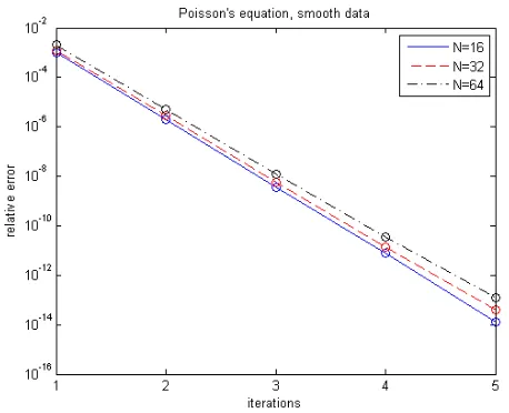
Figure 1: Relative error in solutions to Poisson’s equation (20), (21), (22) computed by 2-node block KSS methods with residual correction.

The coeﬃcient 𝑝(𝑥, 𝑦) is constructed so as to have the smoothness of a function with four continuous deriva-tives, using a technique described in [16]. The function

𝑓 is obtained by applying the spatial operator 𝐿𝑢 = −∇ ⋅(𝑝∇𝑢) to a function 𝑢(𝑥, 𝑦) that is constructed in the same was as 𝑝(𝑥, 𝑦), with the same smoothness, so that the exact solution is known.

In our experiments, we will use diﬀerent grid spacings in order to investigate how the error varies with increasing resolution. The problem data is computed on the ﬁnest grid, and projected onto the coarser grids. However, in order to isolate error due to KSS methods themselves, we do not include error due to truncation of Fourier series in our error estimates.

The results are shown in Figure 1 and Table 1. The rel-ative error is rapidly reduced by residual correction until it is not much greater than machine precision. As shown in the ﬁgure, we achieve linear convergence, with a very small asymptotic error constant. We also see that the error only increases by a factor of 3 as the number of grid points per dimension doubles, but these error estimates do not include truncation of Fourier series. As will be seen in later experiments, the overall error decreases as the number of grid points increases, as expected.

We now solve (20) with a less smooth coeﬃcient and right-hand side,

𝑝(𝑥, 𝑦) ≈ 4.04 + 0.017 cos𝑦+ 0.0052 sin𝑦+ 0.0089 cos 2𝑦+ 0.0042 cos 3𝑦+

(5)

[image:5.612.314.538.75.259.2]

Table 1: Relative 𝐿2 error, excluding truncation of Fourier series, in solutions of (20), (21), (22) with𝑁 grid points per dimension. The third column lists the number of iterations of residual correction.

𝑁 Error Iterations 16 1.3e-14 4 32 4.0e-14 4 64 1.2e-13 4

0.014 sin𝑥+ 0.0083 cos(𝑥+𝑦) +

0.0036 cos(𝑥+ 2𝑦) + 0.0023 cos(𝑥+ 3𝑦) +

0.0066 cos(𝑥−2𝑦) + 0.0073 cos(𝑥−𝑦) + 0.0046 sin(𝑥−𝑦) + 0.0072 cos 2𝑥+ 0.0038 cos(2𝑥+𝑦) + 0.0018 sin(2𝑥+𝑦) +

0.004 cos(2𝑥−𝑦)−0.0034 sin(2𝑥−𝑦) + 0.004 cos 3𝑥+ 0.0033 cos(3𝑥+𝑦) +

0.0026 cos(3𝑥−𝑦), (23)

𝑔(𝑥, 𝑦) ≈ −2.39 sin𝑦+ 4.93 sin 2𝑦+ 3.82 sin 3𝑦− 0.31 sin𝑥−1.44 sin(𝑥+𝑦) +

0.68 sin(𝑥+ 2𝑦)−1.37 sin(𝑥+ 3𝑦)− 0.98 sin(𝑥−3𝑦)−5.75 sin(𝑥−𝑦)− 1.78 sin 2𝑥−1.15 sin(2𝑥+𝑦)− 1.21 sin(2𝑥+ 2𝑦)−1.67 sin(2𝑥+ 3𝑦)− 0.24 sin(2𝑥−3𝑦) + 0.95 sin(2𝑥−2𝑦)− 0.12 cos(2𝑥−𝑦)−5.47 sin(2𝑥−𝑦) + 0.34 cos 3𝑥+ 8.84 sin 3𝑥+

0.19 cos(3𝑥+𝑦) + 4.95 sin(3𝑥+𝑦) +

2.3 sin(3𝑥+ 2𝑦)−1.84 sin(3𝑥+ 3𝑦) + 0.72 sin(3𝑥−3𝑦) + 0.79 sin(3𝑥−2𝑦) + 0.98 sin(3𝑥−𝑦), (24)

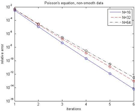
and with Dirichlet boundary conditions. The results are shown in Figure 2 and Table 2. We observe that even though the Fourier coeﬃcients of the problem data decay more slowly than in the previous problem by two orders of magnitude, the computed solution has comparable ac-curacy, after just one extra iteration of residual correc-tion. As before, the error increases only moderately as the number of grid points per dimension is doubled.

3.2 A Multigrid Approach

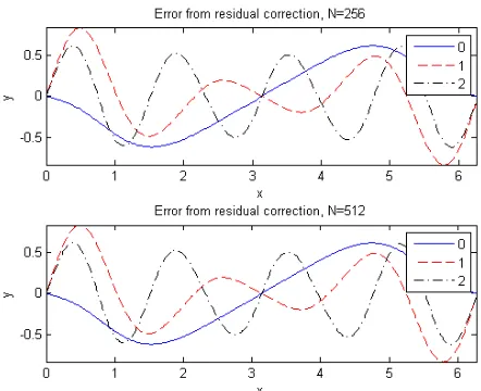
Figure 3 displays the error in solutions to a one-dimensional analogue of (20) with smoothly varying co-eﬃcients and data, after each pass of residual correction, using a 2-node block KSS method with 256 and 512 grid points, respectively. It can easily be seen from the

[image:5.612.369.487.385.436.2]

ﬁg-Figure 2: Relative error in solutions to Poisson’s equation (20), (23), (24) computed by 2-node block KSS methods with residual correction.

Table 2: Relative 𝐿2 error, excluding truncation of Fourier series, in solutions of (20), (23), (24) with𝑁 grid points per dimension. The third column lists the number of iterations of residual correction.

𝑁 Error Iterations 16 6.0e-15 5 32 8.9e-14 5 64 3.1e-13 5

ure, and conﬁrmed by a simple Fourier analysis, that for Poisson’s equation, the error in the initial iterations of residual correction is smooth, but becomes less smooth as residual correction continues. Furthermore, the initial smooth error is essentially independent of the grid reso-lution. Therefore, it makes sense to use a multigrid-like approach, in which initial solutions are computed on a coarse grid, and corrected on a ﬁner grid; that is, the opposite sequence of a traditional V-cycle.

We now try this multigrid-like approach on the following one-dimensional problem

∂ ∂𝑥

(

𝑝(𝑥)∂𝑢

∂𝑥

)

=𝑔(𝑥),) (25)

with Dirichlet boundary conditions, where

𝑝(𝑥) ≈ 4.2206 + 0.2436 cos𝑥+ 0.036459 sin𝑥+ 0.022538 cos 2𝑥−0.0070943 sin 2𝑥+ 0.0019983 cos 3𝑥+ 0.0011086 sin 3𝑥, (26)

(6)

Figure 3: Error in computed solutions to a 1-D ana-logue of (20) after zero (solid blue curve), one (dashed red curve), and two (dotted-dashed black curve) itera-tions of residual correction in conjunction with a 2-node block KSS method on a 256-point grid (top plot) and a 512-point grid (bottom plot).

0.0014578 sin 2𝑥−0.01084 sin 3𝑥. (27)

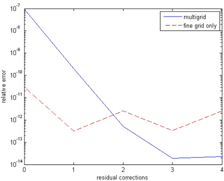
The results are shown in Table 3 and Figure 4. The problem is solved in the following ways:

∙ Performing residual correction on a ﬁne grid contain-ing𝑁 = 1024 grid points

∙ Performing residual correction on a sequence of grids, beginning with a coarse grid containing only

𝑁 = 32 grid points, and then reﬁning to 𝑁 = 64,128,256,512,and ﬁnally 1024 grid points.

In both cases, a 2-node block KSS method is used, as be-fore. Error is measured by comparing the discrete Fourier transforms of each approximate solution to that of the ex-act solution on the ﬁnest grid. We observe that except for a couple of iterations, the error in the two methods is nearly identical, and in all cases it is comparable, but of course the multigrid scheme is much more eﬃcient due to its use of coarser grids.

3.3 The Helmholtz Equation

Now, we apply a 2-node block KSS method to the inho-mogeneous Helmholtz equation

Δ𝑢(𝑥, 𝑦) +𝑘(𝑥, 𝑦)2𝑢(𝑥, 𝑦) =𝑔(𝑥, 𝑦), (28)

with periodic boundary conditions, where

[image:6.612.59.280.75.255.2]

𝑘(𝑥, 𝑦)2 ≈ 4.0901 + 0.0054715 cos𝑦+

Table 3: Relative error in solutions to Poisson’s equa-tion (25), (26), (27) computed by 2-node block KSS methods with residual correction, on multiple grids with

𝑁 = 32,64,128,256,512,1024 grid points, and a single grid with𝑁 = 1024 grid points.

Method 𝑁 Corrections Error

32 0 9.973e-3

64 1 1.271e-4

Multigrid 128 2 2.403e-6 256 3 8.331e-8 512 4 7.228e-9 1024 5 1.182e-11 1024 0 1.088e-2 1024 1 1.470e-4 Fine grid only 1024 2 2.543e-6 1024 3 4.725e-8 1024 4 7.582e-10 1024 5 1.402e-11

0.0016952 sin𝑦+ 0.0060875 cos𝑥+

0.00039064 sin𝑥+ 0.0013668 cos(𝑥+𝑦)− 0.00069206 sin(𝑥+𝑦) +

0.0011185 cos(𝑥−𝑦), (29)

𝑔(𝑥, 𝑦) ≈ 0.41002 + 0.0069992 cos𝑦− 0.0017691 sin𝑦+ 0.004967 cos𝑥+

0.0029314 sin𝑥+ 0.0025509 cos(𝑥+𝑦)− 0.0001331 sin(𝑥+𝑦) +

0.00069903 cos(𝑥−𝑦)−

0.00059274 sin(𝑥−𝑦). (30)

The coeﬃcient𝑘(𝑥, 𝑦)2_{is shown in Figure 5. The results}

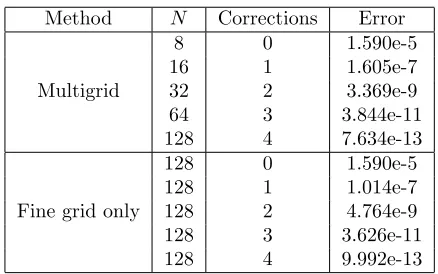
are shown in Table 4 and Figure 6. We observe even more accuracy than in the previous experiment for Poisson’s equation, and even more agreement in the error between the multigrid and single-grid methods.

Generally, the dominant portion of the error arises from the computation of the Fourier coeﬃcients corresponding to the region of phase space where the symbol of 𝐿 = Δ +𝑘2 _{is smallest. This leads to Gaussian quadrature}

nodes near the singularity in the integrand 𝑓(𝜆) =𝜆−1_.

The integrand is more diﬃcult to approximate accurately by polynomial interpolation near this singularity, and the resulting error is negligibly impacted by grid reﬁnement.

However, this error is substantially reduced if the coeﬃ-cient𝑘(𝑥, 𝑦)2_{and right-hand side}_𝑔₍_{𝑥, 𝑦}_{) are very smooth,}

[image:6.612.315.541.149.306.2]

(7)

pre-Figure 4: Relative error in solutions to Poisson’s equation (25), (26), (27) computed by 2-node block KSS meth-ods with residual correction, on multiple grids with𝑁 = 32,64,128,256,512,1024 grid point (blue solid curve) and a single grid with 𝑁 = 1024 grid points (red dashed curve).

conditioning similarity transformations, aided by fast al-gorithms presented in [3] for application of Fourier inte-gral operators, for homogenizing variable coeﬃcients in order to improve the performance of KSS methods for such problems.

Table 4: Relative error in solutions to the Helmholtz equation (28), (29), (30) computed by 2-node block KSS methods with residual correction, on multiple grids with

𝑁 = 8,16,32,64,128 grid points per dimension, and a single grid with 𝑁= 128 grid points per dimension.

8 0 1.590e-5

16 1 1.605e-7 Multigrid 32 2 3.369e-9 64 3 3.844e-11 128 4 7.634e-13 128 0 1.590e-5 128 1 1.014e-7 Fine grid only 128 2 4.764e-9 128 3 3.626e-11 128 4 9.992e-13

Next, we solve the modiﬁed problem

Δ𝑢(𝑥, 𝑦) + 100𝑘(𝑥, 𝑦)2𝑢(𝑥, 𝑦) =𝑔(𝑥, 𝑦), (31)

[image:7.612.319.543.75.260.2]

with periodic boundary conditions and𝑘(𝑥, 𝑦) and𝑔(𝑥, 𝑦)

Figure 5: smooth coeﬃcient𝑘(𝑥, 𝑦)2 in (28) and (31).

as defined in (29), (30). The results are shown in Table 5 and Figure 7. We see that even though there is a greater degree of indefiniteness in the operator 𝐿, the error in the multigrid method is even less than with the smaller coefficient.

In fact, high accuracy is achieved after only a single resid-ual correction. This is because the dominant portion of the error, described earlier, corresponds to Fourier coeffi-cients that, in the exact solution, are significantly smaller. On the other hand, the single-grid approach, while im-mediately yielding high accuracy, is not aided by residual correction. This is because residual correction requires a particularly accurate residual, but at this level of racy, and with no finer grid available, a sufficiently accu-rate residual cannot be computed.

We now solve (28) with less smooth coeﬃcients and data,

𝑘(𝑥, 𝑦)2 ≈ 4.0867 + 0.0054715 cos𝑦+

0.0016952 sin𝑦+ 0.00060255 cos 2𝑦+

0.0060875 cos𝑥+ 0.00039064 sin𝑥+

0.0013668 cos(𝑥+𝑦)− 0.00069206 sin(𝑥+𝑦) +

0.00023799 cos(𝑥+ 2𝑦) +

0.00013712 cos(𝑥−2𝑦)− 0.00013463 sin(𝑥−2𝑦) +

0.0011185 cos(𝑥−𝑦) + 0.00072674 cos 2𝑥+ 0.00031291 cos(2𝑥+𝑦) +

0.00021032 cos(2𝑥−𝑦), (32)

𝑔(𝑥, 𝑦) ≈ 0.41086 + 0.0069992 cos𝑦−

[image:7.612.57.283.77.259.2] [image:7.612.60.279.512.649.2]

(8)

[image:8.612.55.286.77.261.2]

Figure 6: Relative error in solutions to the Helmholtz equation (28), (29), (30) computed by 2-node block KSS methods with residual correction, on multiple grids with

𝑁 = 8,16,32,64,128 grid points per dimension (blue solid curve) and a single grid with 𝑁 = 128 grid points per dimension (red dashed curve).

8 0 9.797e-8

0.004967 cos𝑥+ 0.0029314 sin𝑥+

0.0025509 cos(𝑥+𝑦)− 0.0001331 sin(𝑥+𝑦) +

0.00033062 cos(𝑥+ 2𝑦) +

0.00012874 cos(𝑥−2𝑦) + 0.00069903 cos(𝑥−𝑦)− 0.00059274 sin(𝑥−𝑦) + 0.00081406 cos 2𝑥−

0.00025677 sin 2𝑥+

0.00012879 cos(2𝑥+𝑦) +

0.00018624 sin(2𝑥+𝑦) +

0.00011291 cos(2𝑥−𝑦) + 0.00020258 sin(2𝑥−𝑦) +

0.00012862 cos 3𝑥, (33)

and with periodic boundary conditions. The coeﬃcient

𝑘(𝑥, 𝑦)2_{is shown in Figure 8. The results are shown in}

Ta-ble 6 and Figure 9. We observe that the reduced smooth-ness leads to some loss of accuracy, but the multigrid and single-grid methods still perform comparably. Fur-thermore, the errors are also comparable to that achieved for Poisson’s equation, for which coeﬃcients and data of the same smoothness were used.

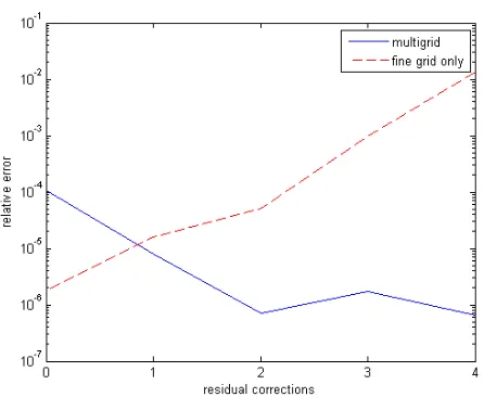
Finally, we solve the same problem, except that the coef-ﬁcient 𝑘2 _{is replaced by 100}_𝑘2_{. The results are shown in}

Table 7 and Figure 9(b). We see that the combination of reduced smoothness and the magnitude of the coefficient poses difficulty for block KSS methods as the number of grid points increases. Due to the reduced smoothness, the dominant portion of the error corresponds to Fourier coefficients that are more significant in the exact solu-tion. Furthermore, because these Fourier coefficients cor-respond to higher frequencies than when𝑘2 _{is relatively}

[image:8.612.314.538.78.259.2] [image:8.612.61.279.438.575.2]

(9)

[image:9.612.68.287.74.261.2]

Figure 8: less smooth coeﬃcient𝑘(𝑥, 𝑦)2in (28) and (31).

8 0 3.488e-4

errors. In fact, the accuracy degradeswhen residual cor-rection is applied on a single ﬁne grid, due to the afore-mentioned inability to obtain an accurate residual, but the multigrid approach is still eﬀective to reducing error, to at least some extent.

4 Summary and Future Work

We have demonstrated that KSS methods, while origi-nally designed for time-dependent PDE, can also be ap-plied to time-independent elliptic PDE with smoothly varying coeﬃcients. Using residual correction on succes-sively ﬁner grids within a multigrid-like framework, these methods can compute highly accurate solutions, even for the Helmholtz equation, for which the integrand in the

8 0 1.077e-4

Riemann-Stieltjes integrals used to compute Fourier co-eﬃcients is singular.

Future work will extend the approach described in this paper to problems in which

[image:9.612.312.538.79.259.2] [image:9.612.60.279.377.511.2] [image:9.612.320.534.437.573.2]

(10)

[image:10.612.59.282.76.259.2]

cancellation of spurious high-frequency oscillations. Our goal is to combine this approach with block KSS methods in order to generalize the superior accuracy of the block approach to these more diﬃcult prob-lems. Alternative approaches may beneﬁt from re-projection techniques (see, for example, [4]) or grid adapation (see [19]).

∙ the domain has a complicated geometry. The main ideas behind block KSS methods are unrelated to the choice of a Fourier basis; they can be applied toany Galerkin method. Ongoing work considers the appli-cation of KSS methods to approximating functions of stiﬀness matrices arising from ﬁnite element dis-cretizations. Another avenue of extension builds on Fourier continuation along lines, as used by Bruno and Lyon [2].

In addition, we will consider the use of Gauss-Radau and Gauss-Lobatto rules, in which selected nodes are pre-scribed, to deal with the singularity associated with the Helmholtz equation.

While the experiments in this paper pertaining to Pois-son’s equation used homogeneous Dirichlet boundary conditions, periodic boundary conditions can easily be used instead, as demonstrated in the examples for the Helmholtz equation, since the eigenfunction correspond-ing to the zero eigenvalue in (20) is known. This problem is of particular interest in the study of mercury emissions

by coal-fired power plants, and their interaction with acti-vated carbon and fly ash, because the intermolecular po-tentials of reactants and products are needed to compute thermodynamic properties in the simulation of power plant conditions. Future work will include the incorpo-ration of block KSS methods into a modified particle-particle, particle-mesh (𝑃3_𝑀_{) algorithm [11] for this}

ap-plication.

References

[1] Atkinson, K.: An Introduction to Numerical Analy-sis, 2nd Ed.Wiley (1989)

[2] Bruno, O., Lyon, M.: High-order unconditionally-stable FC-AD solvers for general smooth domains I. Basic elements. Submitted.

[3] Candes, E., Demanet, L., Ying, L.: Fast Compu-tation of Fourier Integral Operators. SIAM J. Sci. Comput.29(6) (2007) 2464-2493.

[4] Gelb, A., Tanner, J.: Robust Reprojection Methods for the Resolution of the Gibbs Phenomenon.Appl. Comput. Harmon. Anal.20 (2006) 3-25.

[5] Golub, G. H., Meurant, G.: Matrices, Moments and Quadrature.Proceedings of the 15th Dundee Confer-ence, June-July 1993, Griﬃths, D. F., Watson, G. A. (eds.), Longman Scientiﬁc & Technical (1994)

[6] Golub G. H., van Loan, C. F.:Matrix Computations, 3rd Ed.Johns Hopkins University Press (1996)

[7] Golub, G. H., Underwood, R.: The block Lanc-zos method for computing eigenvalues.Mathematical Software III, J. Rice Ed., (1977) 361-377.

[8] Golub, G. H, Welsch, J.: Calculation of Gauss Quadrature Rules.Math. Comp.23(1969) 221-230.

[9] Guidotti, P., Lambers, J. V., Sølna, K.: Analysis of 1-D Wave Propagation in Inhomogeneous Media. Numerical Functional Analysis and Optimization27

(2006) 25-55.

[10] Hochbruck, M., Lubich, C.: On Krylov Subspace Approximations to the Matrix Exponential Opera-tor.SIAM Journal of Numerical Analysis34(1996) 1911-1925.

(11)

[12] Lambers, J. V.: Derivation of High-Order Spec-tral Methods for Time-dependent PDE using Modi-ﬁed Moments.Electronic Transactions on Numerical Analysis28(2008) 114-135.

[13] Lambers, J. V.: Enhancement of Krylov Sub-space Spectral Methods by Block Lanczos Iteration. Electronic Transactions on Numerical Analysis 31

(2008) 86-109.

[14] Lambers, J. V.: An Explicit, Stable, High-Order Spectral Method for the Wave Equation Based on Block Gaussian Quadrature.IAENG Journal of Ap-plied Mathematics38(2008) 333-348.

[15] Lambers, J. V.: Krylov Subspace Spectral Meth-ods for the Time-Dependent Schr¨odinger Equation with Non-Smooth Potentials.Numerical Algorithms in press.

[16] Lambers, J. V.: Krylov Subspace Spectral Meth-ods for Variable-Coeﬃcient Initial-Boundary Value Problems. Electronic Transactions on Numerical Analysis20(2005) 212-234.

[17] Lambers, J. V.: Practical Implementation of Krylov Subspace Spectral Methods. Journal of Scientiﬁc Computing32(2007) 449-476.

[18] Lambers, J. V.: A Spectral Time-Domain Method for Computational Electrodynamics.Proceedings of the IAENG Multiconference of Engineers and Com-puter Scientists(2009) 2111-2116.