The Influence of Inflow Condition on the Generation of Tumbling Flow Using Detached Eddy Simulation

The Influence of Inflow Condition on the Generation of

Tumbling Flow Using Detached Eddy Simulation

Mustapha Mahdaoui1, Abdelouahad Ait Msaad1, Mhmed Mouqallid1, Elhoussin Affad2

1

Laboratory of Mechanics, Energetics and Processes, Ecole Nationale Supérieure d’Arts et Métiers, Moulay Ismail University, Meknes, Morocco

2

Laboratory of Heat and Mass Transfer, FST of Mohammedia, Hassan II University, Mohammedia, Morocco

Email: [email protected]

Received December 2, 2011; revised December 27, 2011; accepted January 12, 2012

ABSTRACT

One of the objectives of car manufacturers is to improve engine performance, reduce consumption reduce emissions. To achieve this objective, it is important to understand the phenomena involved in the combustion chambers of engines. These phenomena are numerous and complex in nature such: the aerodynamics, fuel-air mixture, turbulence, combus-tion and the cycle to cycle instabilities that cause more problems. One of the factors responsible for the phenomenon of cycle to cycle variations is the instability of the characteristics of the vortex flow Tumble. This instability may be due to changes in initial conditions. This study is achieved in order to contribute in a better understanding of engine flow by using a Detached Eddy Simulation Shear-Stress Transport (DES SST) model, which is a hybrid RANS/LES model. These simulations have been performed with the commercial CFD (computational fluid dynamic) code (FLUENT) cou-pled with our own development based on UDF facilities given by FLUENT. To explore the suitability of the 3D DES STT to simulate the internal flow, the calculation is performed for a model tumbling flow at constant volume. This flow has been measured in an experimental set up and measurements are used to initiate and to validate simulations. For this case study, we consider simplified engine geometry. To generate tumbling motion, we use non-reacting DES with a single cycle (SC) strategy. Also, with this strategy we study the effect of initial conditions on the instabilities that ac-company a vortex type tumble.

Keywords: Aerodynamics; Cycle to Cycle Variations; Detached Eddy Simulation; Tumble

1. Introduction

Today, engine designers are seeking very kind of solu- tion aimed at the reduction of fuel consumption and emission levels. Understanding the nature of the flows and combustion in internal combustion engines are im-portant to reach this goal.

Several researchers have been studying that cycle by cycle variations in combustion significantly influences the performance of spark-ignition engines. So, sources of the cycle to cycle variations (ccv) have been intensively studied [1,2]. There are many factors that cause or influ-ence the cycle-to-cycle fluctuations. Taking into account that the cyclic velocity variations are only a part of the more general case of combustion variations, these factors are in detail: mixture composition, geometrical factors, cylinder charging, ignition factors and in-cylinder flow. However, it is more difficult to give a definite conclusion on the nature of dynamics, because ccv is caused by cou-pled effects of a few factors and the influence mecha-nisms of some factors not yet have been clear so far [3,4].

But it is generally accepted that the aerodynamics and the mixing quality are factors that have an important influ-ence on the cycle to cycle variations of combustion.

Experimental studies are more expensive than computa-tional studies. Also using computacomputa-tional techniques al-lows one to obtain all the required data for the cylinder, some of which could not be measured.

bustion systems. The feasibility of using a Detached Eddy Simulation Shear-Stress Transport (DES SST) model, which is a hybrid RANS/LES model, to predict cycle to cycle variations is investigated. Note that the two-equa- tion RANS SST model is used for the near wall region or in regions where the grid resolution is not sufficiently fine to resolve “smaller” structures. In the other regions with higher grid resolution, we adopt the well know LES model [5].

In the context of internal combustion engines, tumble is the name given to a large-scale vortical flow rotating about an axis perpendicular to the piston velocity. Tum-bling flows are generated during the intake phase by the inlet port, the cylinder head and the piston arrangement. Tumble is the flow regime preferred by most modern spark ignition engine designers to enhance compression stroke turbulence. It is now being extensively used on high performance and normal production car engines. Tumble is also critical for the functioning of the new direct inject spark ignition engines, as the combustion in these engines is very lean and requires large amounts of turbulence to stabilize it. In addition, the increased tur-bulence enhances the brief mixing period of the fuel spray before ignition. Hill [6] reported that tumble re-duces cyclic variability and can be an effective technique to improve the thermal efficiency of lean burn engines. However, as the tumble motion increases, heat loss be-comes more significant and the effectiveness of the tum-ble might be more dependent on the ignition process, like spark current intensity and duration.

A literature review of use of computational fluid dy-namics (CFD) codes to model the in cylinder fluid flow, turbulence and spray characteristics was discussed in [7].

Large eddy simulations (LES) are performed in order to reproduce the generation and the breakdown of a tum-bling motion in the simplified model engine by Toledo et al. [8]. The main statistical quantities, such as mean ve-locity and turbulent kinetic energy, are obtained from a set of independent cycles and compared to experiments.

The effect of the inflow condition on the evolution of the flow is tested, with a hyperbolic tangent inflow con-dition producing a markedly different flow-field to a mixing layer initialized from laminar boundary layer profiles given identical flow conditions [9].

In [10], the fluid characteristics of a round turbulent jet flow are studied numerically. The results showed that inflow conditions had a strong influence on the jet char-acteristics.

A single cycle SC strategy has been chosen for this numerical study. A brief overview of the SST-based DES and URANS approaches and their implementation in the FLUENT solver, which is used in this study, is given in the first section. The second part of this paper describes the experimental configuration and measurements.

Nu-merical results are presented and compared to experi-mental data. In the last part we are study the effect of initial conditions on the instabilities that accompany a vortex type tumble.

2. Governing Equations and Turbulence

Modeling

The formulation of the filtered governing equations for mass, momentum and energy equation used in the CFD solver FLUENT are given by [11]:

 

0

i i

t x u

 _

 

(1)

 

 

 





ij ij

i i j

j i j j j

p

u u u

t x x x x x

 

  

        

    

   

_{ }  _{ }  _  _

   

(2)

 













eff j j eff h

j

E E p

t

k T h S

 





 _{   } 

_ 

 

 

      





J 

V

V

(3) 

where ij is the stress tensor due to molecular viscosity defined by

2 3

ij ij

j

i i

j i i

µ µ

x u

u u

x x

  _  _  

  

 _{ }

 

ij

(4)

 is the subgrid-scale stress defined by and

j ij u ui u ui j

   (5)

In Equation (3) k is the effective conductivity ( eff t

eff

k  k k , where kt is the turbulent thermal con- ductivity, defined according to the turbulence model be- ing used), and Jj is the diffusion flux of species j. The first three terms on the right-hand side of Equation (3) represent energy transfer due to conduction, species dif- fusion, and viscous dissipation, respectively. h includes the heat of chemical reaction, and any other volumetric heat sources.

S

The total energy E is defined by:

2

2

p v E h

 (6)   

where, for ideal gases the sensible enthalpy h is defined as

j j j

h



Y h (7)

and for incompressible flows as

j j j

p

h



Y h  (8)

In Equations (8) Yj

, d

ref

T j _T p j h 

_

c T

ref T -k ω -k

is the mass fraction of species j and

(9) where is the reference temperature (=298.15 K).

2.1. The SST Model

In the context of RANS and URANS modelling, there exist a great variety of models for the turbulent viscosity. FLUENT provides large choices of turbulence models, we cite for example the Spalart-Allmaras model [12], the

 models and the k- models, in which k is the tur-bulent kinetic energy (TKE),  is the dissipation of the TKE and  is the specific dissipation of TKE.

The standard k- model in FLUENT is based on the Wilcox k- model [13], the shear-stress transport (SST)

-k models proposed by Menter [14] to effectively blend the robust and accurate formulation of the k-

model in the near-wall region with the free-stream inde-pendence of the -k model in the far field. To achieve this, the k- model is converted into a k- formula-tion.

For the SST k- turbulence model, he transport equations for k and  are given by:

 



i



t

i j k

u k

k µ k

t x x

              _  _

   _ _ _ k k

j k

µ G Y S

x     (10)

 







1



,2

2 1

i t

i j

u µ

t x x

Y F  1 j j j µ G x k _S x x    _           t           _{ }   _          _{ }    (11) where  is the turbulent viscosity

*

2

1 1

1

x ,SF

a ma t k             (12)

where S is the strain rate magnitude and the coefficient

*

 damps the turbulent viscosity causing a low-Reynolds- number correction.

In the high-Reynolds-number form of the k- model,

*

1

 _ 

The blending functions, F1 and F2, are given by

4

2 2

,2 4

k k

y _ D y_

    _{  }    _{ }  _ _     1 500

tanh min max , ,

0.09 F y     _{ }   _{ }  _{ } (13) where 10 ,2 1 1

max 2 ,10

j j k D x x                   

  (14)

2

2

2 500

tanh max 2 ,

0.09 k F y y     _{  }   

 _{  } (15)

_{  } 

 

where _k and  are the turbulent Prandtl numbers

for k and , respectively





,1

1 1 ,2

1 1

k k

k _{F F}

 (16)

    





,1 ,2 1 1 1 1 F F          k S S (17)

and _ are user-defined source terms.

The term _k represents the production of turbulence kinetic energy, and is defined as:

G

*

min i j j,10 k i k u x u u

G     _

       G (18)

The term  represents the production of  and is

given by: i t i j j u u G u x         

 (19)

0 * 1 t t e e R R R R         

   (20)

     where t e k R    -k (21)

For the SST  model, 





1 ,1 1 1 ,2

F F

is given by

_  _   _ (22) where 2 ,1 ,1 * * ,1 i          

  (23)

2 ,2 ,2 * * ,2 i          

  (24)

where  is the Von Kàrmàn constant (=0.41).

The term _k represents the dissipation of turbulence kinetic energy, and is defined in a similar manner as in the standard

Y

-k model.

*

k

Y  k

 

* * *

1

i F Mt

  

(25) where

  (26)

3. Computational Domain









* * 4 15

1 i

 _

 

4 4

t

t

e

e R R

R R





 _ 

 

 

 

 

Y

(27)

The term  represents the dissipation of , and is

defined by

2

Y (28)

where

 

* *

i

i t

i

F M



 

 

 

 

t

1 

 



  (29)

is the compressibility function, F M 0

0

2

t t

t t

, given by

 

0

t t

M M

F M

M M

 

M

    

(30)

2 2

2 t

M k

a



0 0.25

t

M 

(31)

(32) a RT

i

(33)

 is given by





1 1 1 i,2

F1 , F

i i

     

*

*

Y k f

(34) The constants of the model are given in Table 1. (21 cm*28.5 cm).

2.2. The SST DES Model

The dissipation term of the TKE is modified for the DES turbulence model as described in Menter [15] such that:

k   _ (35)

where f_* a constant is no longer equal to 1 as in the URANS SST k- model, but is now expressed as

* max f_ 

C

DES

,1 t L C

 

 _ 

 







max , ,

(36)

where DES is a calibration constant used in the DES

model and is a mesh scale given by: x y z

     (37) The turbulent length scale is the parameter that defines this RANS model:

*

t

k L

 



p The geometry of the computational domain reproduces the compression chamber of Borée et al. [16] (Figure 1). It is composed of a square piston which has a sinusoidal motion, a guillotine to close the flat intake channel, a plenum chamber at ambient pressure and multiple optical accesses for Particle Image Velocimetry (PIV) measure- ments. The piston dimensions are 100 × 100 mm2, The distance between the piston and the cylinder head at the end of the intake stroke is hI = 100 mm. The compression ratio is equal to 4 and the resulting peak pressure ( max)

is about 5, 5 bar. The length to height ratio of the intake channel (L hl30) guarantees that turbulence is fully established when the flow reaches the chamber. During the intake stroke the maximum Reynolds number based on the hydraulic diameter is .

(38)

max

Re 12, 000

4

2 10 s

t 

  

,1 k

4. Numerical Results

The objective of this section is to compare the general flow structure from DES and experiment [16] at the end of intake.

The numerical method used for the present simulations is based on a finite volume discretization of the com- pressible Navier-Stokes equations. The computational grid and the mesh are generated from the GAMBIT software; the computational mesh consists of 731,787 hexahedral cells. The time step is . For all equations of the model, the convection terms are treated with the first-order upwind spatial interpolation scheme. All simulations consider the value of the empirical con- stant (CDES) (in Equation (36)) equal to 0.78.

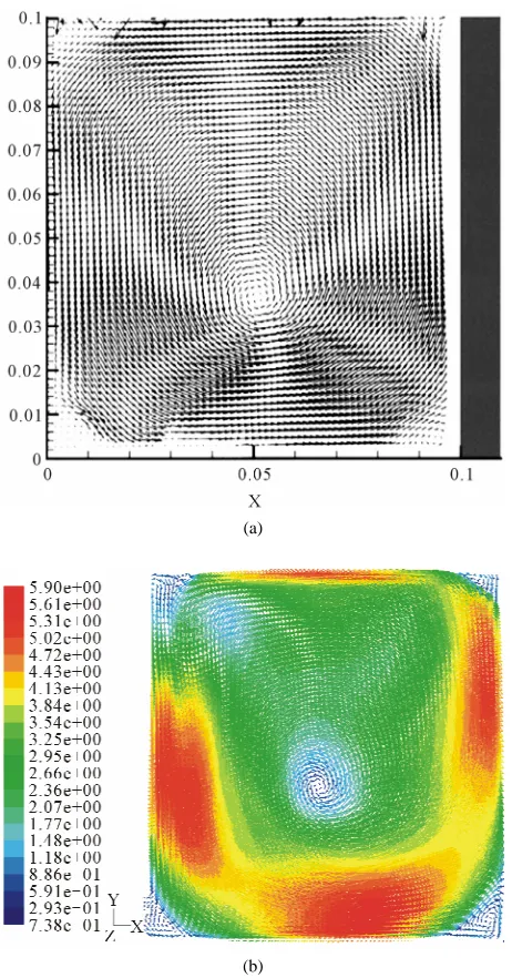
In order to study the influence of the pressure-velocity coupling for a tumble type flow, simulations are done using different algorithms available in FLUENT software such SIMPLE, SIMPLEC and PISO. Figures 2(a) and (b)

show the mean velocity field at the end of intake. At this location, the tumble is correctly predicted with a slight deviation of the vortex core.

Figures 3 and 4 compare the computed (with different algorithms) and measured profiles of the x and y com- ponents. One can see the profiles from the PISO algo- rithm had a good agreement with experiment results.

[image:4.595.52.288.82.388.2]

It is generally accepted that cyclic combustion vari- ability in spark-ignition engines arises from the varia- tions in the quantity, composition of the mixture and the flow characteristics in the engine [1,2]. That is why the effect of inflow conditions on the variations of the char- acteristics of the internal flow engine is studied.

Table 1. The model constants.

 ,1 k,2 ,2 a1 i,1 i,2 0 

*

 R R * M t0

Laser sheet

Piston

Location of guillotine device

[image:5.595.310.536.86.232.2]

Intake channel Windows

Figure 1. Sketch of the experimental setup [16].

(a)

[image:5.595.57.285.86.238.2]

(b)

[image:5.595.58.289.267.708.2]

Figure 2. Mean velocity fields at the end of the intake stroke from experiment (a) and simulation (b) [16].

[image:5.595.311.537.269.453.2]

Figure 3. X-velocity profiles with DES simulation, using different algorithms.

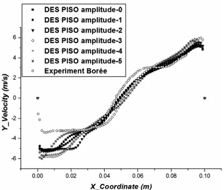
Figure 4. Y-velocity profiles with DES simulation, using different algorithms.

Figures 5 and 6 show a comparison between the com- puted and measured x-velocity and y-velocity profiles using different turbulence intensity on inflow boundary condition. We can observe the sensibility of the model to the turbulence intensities variation especially near the wall.

To study the influence of the inflow velocity fluctua- tions on the internal flow instability, we introduced spa- tial sinusoidal perturbations on the velocity profiles (pro- files with the same period but the different amplitudes for which the mean amplitudes is about 10 m/s). At the end of intake x-velocity and y-velocity profiles are displayed in Figures 7 and 8. From these figures we can note that velocity profiles has an effect of the flow instability.

[image:6.595.308.534.86.278.2] [image:6.595.58.287.87.260.2]

Figure 5. X-velocity profiles with DES simulation, using different turbulence intensities.

Figure 6. Y-velocity profiles with DES simulation, using dif-ferent turbulence intensities.

Figure 7. X-velocity profiles with DES simulation, using different sinusoidal velocity profiles.

Figure 8. Y-velocity profiles with DES simulation, using different sinusoidal velocity profiles.

[image:6.595.57.287.305.479.2]

not excess 5 mm. Precession of tumble due partly to the effect of movement of the piston, and the other by varia- tions of inflow conditions. Then the inflow conditions for the experience vary from cycle to cycle randomly.

Figure 10 shows variations of the area of the corner vortex for the DES simulations with variation of the ve-locities profile. We can observe changes in the area of the corner vortex. This variation ranges from 0.00003 m2 for profile has amplitude 3 and 0.00035 m2 for profile has amplitude 5.

From these results, we see clearly that the instabilities of tumble velocity profiles at BDC passing through the geometric centre of the chamber, the instabilities of posi-tion of the centre of tumble (precession) and the varia-tions of area of the corner vortex. These variavaria-tions are due to slight variations of the boundary conditions like turbulence intensity and to natural instabilities of the bidimensional intake jet. These differences in position of the central vortex and velocity profiles from cycle to cy-cle are random and unavoidable.

5. Conclusions

This paper shows that the behavior of internal flows en-gines must be studied to improve engine performance in order to reduce consumption and emissions.

Generation of tumbling flow was simulated by using the commercial package FLUENT coupled with our own UDF development. The use of an experimental database achieved to validate the DES SST turbulence model demonstrate that the DES SST is potentially more ada- pted to study the generation of tumbling flow.

[image:6.595.56.286.525.701.2]

[image:7.595.59.285.82.248.2]

Figure 9. Variation of the position of Tumble with fluc- tuations velocities inlet. PIV data from Marc [17].

Figure 10. Variation of the area of the corner vortex with fluctuations velocities inlet.

profiles and turbulence intensity variations on flow field characteristics is considered. The results showed funda- mental differences, especially in the instabilities of tumble velocity profiles at BDC passing through the geometric centre of the chamber, the instabilities of position of the centre of tumble (precession) and the variations of area of the corner vortex.

As a perspective of this work, we will introduce random instead sinusoidal variations on the velocities profiles to study the instability of the vortex flow by DES approach.

REFERENCES

[1] N. Ozdor, M. Dulger and E. Sher, “Cyclic Variability in Spark Ignition Engines,” A Literature Survey, SAEPaper 950683, 1994

[2] J. B. Heywood, “Internal Combustion Engine Fundamen-tals,” McGraw-Hill, New York, 1998.

[3] P. G. Hill, “Cyclic Variations and Turbulence Structure in Spark-Ignition Engines,” Combustion and Flame, Vol. 72,

No. 1, 1988, pp. 73-89.

doi:10.1016/0010-2180(88)90098-3

[4] M. B. Young, “Cyclic Dispersion in the Homogene-ous-Charge Spark-Ignition Engine,” A Literature Survey, SAE Paper 810020, 1981.

[5] J. K. Ball, “Cycle-by-Cycle Variation in Spark Ignition Internal Combustion Engines,” PhD Thesis, Department of Engineering Science, Merton College, Oxford, 1998.

[6] C. Hasse, V. Sohm and B. Durst. “Detached Eddy Simu-lation of Cyclic Large Scalefluctuations in a Simplified Engine Setup,” International Journal of Heat and Fluid Flow, Vol. 30, No. 1, 2009, pp. 32-43.

doi:10.1016/j.ijheatfluidflow.2008.10.001

[7] S. A. Basha and K. R. Gopal, “In-Cylinder Fluid Flow, Turbulence and Spray Models—A Review,” Renewable and Sustainable Energy Reviews, Vol. 13, No. 6, 2008, pp. 1620-1627. doi:10.1016/j.rser.2008.09.023

[8] M. S. Toledo, L. Le Penven, M. Buffat, A. Cadiou and J. Padilla, “Large Eddy Simulation of the Generation and Breakdown of a Tumbling Flow,” International Journal of Heat and Fluid Flow, Vol. 28, No. 1, 2007, pp. 113- 126. doi:10.1016/j.ijheatfluidflow.2006.03.029

[9] W. A. McMullan, S. Gao and C. M. Coats, “The Effect of Inflow Conditions on the Transition to Turbulence in Large Eddy Simulations of Spatially Developing Mixing Layers,” International Journal of Heat and Fluid Flow, Vol. 30, 2009, pp. 1054-1066.

doi:10.1016/j.ijheatfluidflow.2009.07.005

[10] E. Faghani, S. D. Saemi, R. Maddahian and B. Farhanieh, “On the Effect of Inflow Conditions in Simulation of a Turbulent Round Jet,”Archive of Applied Mechanics, Vol. 81, No. 10, 2011, pp. 1439-1453.

doi:10.1007/s00419-010-0494-8

[11] FLUENT 6.3 Documentation, “User’s Guide,” Fluent Inc., 2006.

[12] P. Spalart and S. Allmaras, “A One-Equation Turbulence Model for Aerodynamic Flows,” Technical Report AIAA- 92-0439, American Institute of Aeronautics and Astro-nautics, 1992.

[13] D.C. Wilcox, “Turbulence Modeling for CFD,” DCW Industries, 1993.

[14] F. R. Menter, “Zonal Two-Equation k-ω Turbulence Models for Aerodynamic Flows,” AIAA Paper, 1993. [15] F. R. Menter, M. Kuntz and R. Langtry, “Ten Years of

Experience with the SST Turbulence Model,” In: K. Hanjalic, Y. Nagano and M. Tummers, Eds., Turbulence, Heat and Mass Transfer, Begell House Inc., West Redd- ing, Vol. 4, 2003, pp. 625-632.

[16] J. Boreé, S. Maurel and R. Bazile, “Disruption of a Com-pressed Vortex,” Physics of Fluids, Vol. 14, No. 7, 2002, pp. 2543-2556. doi:10.1063/1.1472505

[image:7.595.60.284.283.448.2]