Stochastic Orders Comparisons of Negative Binomial Distribution with Negative Binomial—Lindley Distribution

(1)

Stochastic Orders Comparisons of Negative Binomial

Distribution with Negative Binomial—Lindley Distribution

Chookait Pudprommarat, Winai Bodhisuwan

Department of Statistics, Kasetsart University, Bangkok, Thailand Email: [email protected]

Received January 20, 2012; revised February 18, 2012; accepted March 4, 2012

ABSTRACT

The purpose of this study is to compare a negative binomial distribution with a negative binomial—Lindley by using stochastic orders. We characterize the comparisons in usual stochastic order, likelihood ratio order, convex order, ex-pectation order and uniformly more variable order based on theorem and some numerical example of comparisons be-tween negative binomial random variable and negative binomial—Lindley random variable.

Keywords: Stochastic Orders; Negative Binomial Distribution; Negative Binomial—Lindley Distribution

1. Introduction





_

_

















The negative binomial (NB) distribution is a mixture of Poisson distribution by mixing the Poisson distribution and gamma distribution. The NB distribution is em-ployed as a functional form that relaxes the overdisper-sion (variance is greater than the mean) restriction of the Poisson distribution (see [1]). If X denote a random variable of NB distributed with parameter r and p then its probability mass function is in form

 

r x

f x _  1_{p 1 p}r



_



x

 _x 

 

0 p 1 

, x 0,1, 2, ,

  



for r 0 and , with E X r 1 p p



 and

  

2



r 1 X

p



 p

Var .

The negative binomial—Lindley (NB-L) distribution which is a mixed negative binomial distribution obtained by mixing the negative binomial distribution with a Lind- ley distribution. The NB-L distribution was introduced by Zamani and Ismail in [2] and it provides a model for count data of insurance claims. If Y is a NB-L random variable with parameter r and  then its probability mass function is in form

 









2 y

j

r y 1 y

g y _   _



 _{ } 1 ₂

j 0

r j 1

y j r j

   

    

   

r 0

,

y 0,1, 2, , for and   , with

 







3

r

1 1



  2 r 1

 

E Y , when  

 

, and













 



2 2 2 3

2 2

2 2 2 3

2

2 4

r r 1 2r r

Var Y

1 2 1 1

r 1 1

r ,

1 1

  

   

  

 

  

 

   

  

 

 

2

when 

 

.



In this respect, the aim of this work is to compare a negative binomial distribution with negative binomial— Lindley distribution base on stochastic orders such as usual stochastic order, likelihood ratio order, convex or-der, expectation order and uniformly more variable order.

2. Stochastic Orders

Stochastic orders are useful in comparing random vari-ables measuring certain characteristics in many areas. Such areas include insurance, operations research, queu-ing theory, survival analysis and reliability theory (see [3]). The simplest comparison is through comparing the expected value of the two comparable random variables. The following, we will define some notions of the sto-chastic orders which will be used in the context of the paper. For more details, we refer to Ross [4], Misra [5], Shaked [6,7] and Singh [8].

Definition 1.Let X and Y be random variables with

densities f and g, respectively, such that g k f k

 

is

non-decreasing function in k over the union of the

sup-ports of X and Y, or, equivalently,

       

f u g v f v g u u v

lr

X Y

, for all . Then X is smaller

than Y in the likelihood ratio order which is denoted by

(2)

Definition 2. Let X and Y be two random variables

such that , for all . Then

X is smaller than Y in the usual stochastic order which is

denoted by .





Pr Y k

X Y



X k



Pr

  k

 





E Y

  

st

such that , for every real valued

convex function

 





E X

 where expectations are assumed to

be existed. Then X is smaller than Y in convex order

which is denoted by cx .

such that , where expectations are

as-sumed to be existed. Then X is smaller than Y in the

ex-pectation order which is denoted by .

X Y

 

X

 

Y

E E

X Y



   

E

with densities f and g, respectively. Recall that supp(X)

and supp(Y) denote the respective support of X and

re-spective support of Y, such that supp(X) supp(Y)

and the ratio f k g k

uv

X Y









is a unimodal function over

supp(Y). Then X is smaller than Y in uniformly more

variable order which is denoted by .

3. Comparison

We make comparisons between the negative binomial random variable and negative binomial—Lindley random variable with respect to the likelihood ratio order, sto-chastic order, convex order, expectation order and uni-form more variable order. The following lemma will be useful in proving the main results.

Lemma 1. Define,

 









k 1

j

j 0

k

j

j 0

k 1 1 j a k 1

k ( 1) j







 

 



 

 

 

      



2

r j 1 r j r j 1 r j

 



       

 

and

 

j 1 r

1

m  m 1 m_  _

 

k 0,1, 2,  a k





k 0,1, 2,



2,



_k

 

m

k 0,1, 2, 

k

j 0

j r j



  

 

 

 



,

m

 , 0 m 1  , Then,

 

1) is a non- increasing function of ,

2) For each fixed , is concave function of .

k 0,1,

 

m 0,1

Proof.

1) We may write for a k

 

, that

 

















 

k

d

E W d





 



 



  





 

h 

k 1 r

0

k r

0

e 1 e h ;

a k 1

e 1 e h ;

 

 



,

where is the Lindley distribution defined by

 

2



_{z e}



z

h z; 1

1

 



 and 0

  , z 0 

and Wk is a random variable havin proba ility

density function:

g the b

 









 









k rz z k _k

1 e 1 e h z;

z ₂

j

2 j 0

k r j 1

( 1)

j _{r j}

 



 

 



   

 

   

 

   



, z 0 .

For fixed k



0,1, 2,



, the ratio _{k 1}

 

x _k

 

x

is obviously a non-increasing function of x 0 . Then, by Definitions 1 and 2, we have Wklr Wk 1 , which yields W_k_st W_{k 1}_ and therefore E W

 

_k E W



_{k 1}



or, equivalently, a k

  

a k 1



. This proves a k

 

is a non-increasing function of k



0,1

2) For k 0



, 2, .

 , note that 

 

m m is both ex and concave. For k 1, 2, 0

conv  , we can write



 

j 1

j

 

r k

j k 1

j r 1

m 1 m 1 m , m, 0 m 1.

 

   

 

  __  __   

 



 

 

(1) The relationship between negative binomial and beta probabilities is of the form





j

_



_{ }



_

1 p





r 1

r k 1

j k

k r 1 ! r r 1

0

p 1 p t 1 t dt

j k



 



   

 

  

  _ _

 





,

1 ! r 1 !



k 0,1, 2, .

Therefore, k

 

m in Equation (1) can be written as





_



_





1 r

1 m 0

m 1

  

m

r 1 k

k

k r !

t 1 t dt k! r 1 !

  





,

, 0 m 1

   .

Thus,









 

k 1

1 1

2 ₁

r r

k

k r ! 1

m m 1 m 0

r r 1 !r!



  



2

m 



  _  _ 

 _ _ ,

m



, 0 m 1

   .

which proves concavity. □

Theorem 1. Let X ~ NB r, p

 

, Y ~ NB-L r,

 

 and











2

r 2 r p0   3

r 1

 

  ,





1

2 r

1 2

r 1 p

r

  

 _{ } 

  



 

 

,







2

2 3

1 1

p  



 

 . Th 0 p 2p1p01

Furthermore, 1) X lr Y

en .

if and only if pp0,



2) Xst Y if and only if p p 1,

3) X _E

 

E Y if and only if p

 

p2, of.

he likel tw n Y and X can be written as

  Pro

(3)

 



_



_

 











 



2 k k r

k r j 1

,

X k _{p 1 p} ₁

k 0,1, 2, .

              (2)

By Definition 1, we have













j 2 j 0 1 j

Pr Y k r j

l k Pr           



  



 

  







 



 

lr k 1 j j 0 k j j 0 0

X Y l k l k+1 , ,



2

0,1, 2, ,

1 r j 1

1

r j

p 1 ,

k r j 1

1

j r j

p a k , , 0,1, 2, , p p a 0 .

k k k k                              _             



 

Since



k+ j  _ 





a k is non-increasing in k (by part 1) in e , then 0

L mma 1) p p which provides a necessary and conditio for the

sufficient n l k

 

in Equation (2) to be o

b

n n-decreasing. This completes the proof of the result. 2) Let Xst Y y Definition 2, we have

























2 r 2 r 1

Pr Y 0 Pr X 0 p ,

r            1 2 r 1 2 r 1

p p . r     _{ }          

Conversely, suppose that 0 p 1 p 1.

k 0













For ,1, 2,, consider

 









 





k i r i 0 2 k i j 2 i 0 j 0

i r 1

k p 1 p

r j 1 i r 1 i

1 ,

i j 1 r j

             _ _    _ _{ } _ _{ } _{  }   _ _ _{ }            



X ~ X ~ NB r, p



1



, then

1 Xst X1.

q



k i 1 1 1

p k Pr X k Pr Y _i

and if

lr

X X

Conse

 

NB r, p and nce, we get

ly, . He uent







k i r r

i 0 i 0

i r 1 i r

p 1 p p 1 p

i _  i 



  



k k

              ,



 

p  p .

For fixed









and therefore

1





k 0,1, 2, ,

1 2 r 2 r 1 r     _{ }         , 1 p 

 

p exp  and ~ Lindley

 

 . We get





 





 









1 k

k



pr  i

p 1 1

i 0

k i _j

2 i 0 j 0

1 p i

r j 1 i r 1 i

1 ,

i j _ ₁ _ _{r j}

     _ _          _ _ _{ }            



 



 











1 i 1 k

r r r p i 0 k i r i 0

i r 1

k E P 1 E P

i i r 1

E P 1 P , i                  _ _      _ _   



Using concave function (by part 2) in Lemma 1),

 

1

p k

 can be written as

 



 

 

 



1

r r

p k k E P E k P

   .

Applying Jensen’s inequality to concave function, we have _



_{E P}

 

r

 

__E _

 

_Pr



_and_

 

_k _₀_for

2

 

 _{ } _{ }

i r 1 

 

k k p₁

k

 , k



0,1, 2,



. Conversely, where Xst Y

at

im-plies th Pr Y 0







Pr



X 0



. This proves p p 1.

3) The proofs of the results are obvious. □ Theorem 2. Suppose that, for every 0 t 1  ,



t p 1



Pr   0, then

1) No value of 0 p 1  can ensure that Xst Y,

2) XuvY if and only if 0 p p  11.

Proof.

1) We find

 









Pr X k

0,1,



R k

Pr Y k



 , k , b

tor and

2, y re-

fr d owing:













 



ying the numera enominator as foll







_{    }















 















j r j k 1 p r 1

k 1 r 1

0 r

k 1 p ,

j k r 1 !

t 1 t dt, k 1 ! r 1 !

1 p 1 t dt, k 1 ! r 1 !

1 p 1 p k r 1 !

.

k 1 ! r 1 ! r 1 p

k                          



For any 0 p p1 1

k 1

   0

1 p

k r 1 !_{ } 

j r 1 p

 _ _{ } _





_ _

Pr X

   , k 0,1, 2, ,





 































 







2 i j 2 i k j 0

i r 0 i r i k 0 1 e r 1 k 1 0

r j 1 r i 1 i

Pr Y k 1 ,

i j r j

r i 1

e 1 e h ; d ,

i r i 1

e 1 e h ; d ,

i

k r 1 !

t 1 t dt

k 1 ! r 1 !

                             _ _{ } _ _{ } _{  }    _ _ _{ }          

i k         __ _  _                        



















 



 















 







0 1 log 1 t 1 r 1 k 1 0 0 1 r 1 k 1 0

h ; d ,

k r 1 !

t 1 t h ; d dt,

k 1 ! r 1 !

k r 1 ! 1

t 1 t H log ; dt,

k 1 ! r 1 ! 1 t

(4)

[image:4.595.57.536.100.220.2]

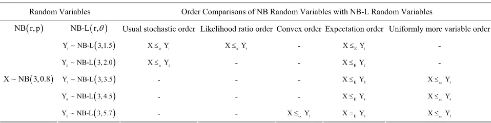
Table 1. Stochastic orders comparisons of NB random variables with NB-L random variables.

Random Variables Order Comparisons of NB Random Variables with NB-L Random Variables

 

NB r, p NB-L r,  Usual stochastic order Likelihood ratio order Convex order Expectation order Uniformly more variable order

  B-L 3,1.5

1

Y ~ N st XlrY5 XEY1 -

2

Y ~ N XstY2 XEY2 -

 

3

Y ~ NB-L 3, 3.5 - - - XEY3 XuvY3

 

4

Y ~ NB-L 3, 4.5 - - - XEY XuvY4

 

5

Y ~ NB-L 3, 5.7 X_EY XuvY5

1

X Y -

 

B-L 3, 2.0 - -

4

 

X ~ NB 3,0.8

- - XcxY5 5

where H

 

 is cumulative distribution function of Lindley distribution:

 

1 z_e z

1 H z; 1   

   

 , z 0 and 0

     .













_

_{ }

_





















1

1 p

r 1 1

k r 1

1 1

k r 1 !

Pr Y k H dt,

1 ! H p ; p

1

k

t

 

 

  

 

_





1 1

0 k 1 ! r 1 ! 

p ; p

r k 1 ! r



 

1

1 p .



k  

! k



So,

 







k

r 1

1 1

p _{1 p}

R k

1 p r 1 p p H p ; 

  

 _ _



 _ _ .





r

1

k 1

Since







k r

1 1

k 1 p _{1 p}

lim 0

1 p r 1 p p H ; 

 _ _ _

  _ 

 _ _ , we have

then



r 1 k

1

p



klim R k 0,   p1 p 1.

lidates the result. ose that The part 2) in

2, it is clear that ran-dom d Y are not ordered by the usual sto-chast from the arguments used in the proof of pa 1, since 0

Ther t follows that, for any 0 p 1  , there ex-ists a sufficiently large k such that







Pr X k Pr Y k efore, i



. This va

1

0 p  p

rt 1) in Theorem 2) Supp

Theorem

1. n, from 1 and pa

variables X an ic order. Also,

rt 1) in Theorem p p it follows that



 



Pr s non-increasing and unimodal, hat . The converse part follows by

mi nts. □

hat 2

X k Pr Y k  i

uv

X Y

lar argume Suppose t implying t

using the si

Theorem 3. p p . Then,

uv

 2) Xcx Y

ows from part 2) in Theorem 2, we ha , where 1

1) X Y

.

Proof.

1) Foll ve

uv

X Y p₂p .

uv

X Y and 2) Since

 











_{ }

3 2

r 1 r

E Y r X

p

1 1



 

  

  ,

p E

 

by ed in [4], X

with negative binomial—Lindley random variable in usual stochastic order, likelihood ratio order, convex or-der, expectation order and uniformly more variable order and the results are provided in Table 1.

Then, we explain that negative binomial random vari-able (X) is smaller than negative binomial—Lindley ran-order implies that X Y

dom variable (Y) in the usual stochastic

E . In addition, if X and Y have respective

supp(X)  supports supp(X) and supp(Y), such that

supp(Y) and the ratio Pr X



k Pr Y k

 





is a uni-modal fun tion over supp but X and Y e not or-dered in t usual stochast order. Furtherm re, if X and Y have a same mean. Then XuvY impl that

cx

X Y

c he

(Y) ic

ar o ies

 .

4. Conclusion

This paper sh ws stochast orders compariso f nega-tive binomial random variable with a neganega-tive binomial—

, ex d

uniformly more variab compari

inomial—Lindley random

va negati ial random

va le (X) is smaller than negative binomial—Lindley ra m variab (Y) in the usual stochastic order. Its us is that it gives a simple sufficient condition for

X xt, if

supp(X) (Y) is t t it implies that the ratio

o ic n o

Lindley random variable by usual stochastic order, like-lihood ratio order, convex order pectation order an

le order. Some advantages of sto-chastic orders son between negative binomial random variable and negative b

riable are as follows: If ve binom riab

ndo le

efulness

is smaller than Y in the expectation order. Ne  supp ha



 



the result of Shak cx Y.

Next, We shows some numerical examples of the comparisons between negative binomial random variable

Pr X k Pr Y k nimodal function over supp(Y) but X and Y are not ordered in the usual stochastic r. Finally, If X and Y have a same mean, it is known X is smaller than Y in uniformly more variable order im-n coim-nve rder. This con-cl

R

is a u

orde that

plies that X is smaller than Y i x o usion is supported by numerical examples.

5. Acknowledgements

We are grateful to the Commission on Higher Education, Ministry of Education, Thailand, for funding support under the Strategic Scholarships Fellowships Frontier

[image:4.595.58.285.258.441.2]

(5)

REFERENCES

[1] W. Rainer, “Econometric Analysis of Count Data,” 3rd Edition, Springer-Verlag, Berlin, 2000.

[2] H. Zamani and N. Isma al—Lindley Distribution and Its Application,” Journal of Mathematics and Statistics, Vol. 6, No. 1, 2010, pp. 4-9.

il, “Negative Binomi

doi:10.3844/jmssp.2010.4.9

[3] M. Shaked and J. G. Shanthikumar, “Stochastic Ord Academic Press, New York, 2006.

Stochastic Processes,” Wiley, New York, ers,”

[4] S. M. Ross, “ 1983.

[5] N. Misra, H. Singh and E. J. Harner, “Stochastic Com-parisons of Poisson and Binomial Random Variables with Their Mixtures,” Statistics and Probability Letters, Vol.

65, No. 4, 2003, pp. 279-290. doi:10.1016/j.spl.2003.07.002

[6] M. Shaked, “On Mixtures from Exponential Families,” Journal of the Roy

No. 2, 1980, pp. 192-198. al Statistical Society: Series B, Vol. 42,

[7] M. Shaked an “Stochastic Orders

and Their Ap Press, New York,

fe Distributions,” d J. G. Shanthikumar,

plications,” Academic 1994.

[8] H. Singh, “On Partial Orderings of Li

Naval Research Logistics, Vol. 36, No. 1, 1989, pp. 103- 110.