An Optimization Method for an Aircraft Rear-end
Conceptual Design Based on Surrogate Models
Sergio de Lucas, Angel Velazquez, and Jose M. Vega
Abstract—A new conceptual design method is presented that is based on the minimization of a target function subject to some restrictions using surrogates. Specifically, the surrogates are used to speed up the calculation of both the various ingredients of the target function and the restrictions. The surrogates are based on a combination of high order singular value decomposition (resulting from a set of snapshots that are calculated using a computational fluid dynamics solver) and modal interpolation. The method is both flexible and much more computationally efficient than the conventional method, especially if the number of design parameters is large. The method is illustrated considering a simplified version of the conceptual design of an aircraft empennage.
Index Terms—Conceptual design, high order singular value decomposition, optimization, surrogate models, reduced order models.
I. INTRODUCTION
C
ONCEPTUAL design in industry is evolving in two conflicting directions: (a) the number of design and tunable modeling parameters keeps increasing, but (b) the time span allocated to the design cycles is being shortened. The difficulty is even deeper since the parameters are of a highly multidisciplinary nature, which means that a set of essentially different Physics/Mathematics modeling equa-tions must be considered. Conceptual design is becoming increasingly dependent of mathematical methods.Many documents have been written on multidisciplinary optimization in conceptual design and on the integration of surrogate models in this. Kroo et al. [1] decompose the problem into two levels: a system level whose responsibil-ity is the coordination of the optimization process, and a lower level made up of sub-spaces for the various technical disciplines. Antoine and Kroo [2], [3] linked the different technical disciplines of engine performance, using a Nelder-Mead [4] algorithm in reference [2] and a genetic algorithm in reference [3]. It is also worth mentioning the applications by Schumacher et al. [5] on the structural design of a wing box, by Piperni et al [6] on the design of business jets, and by Queipo et al. [7] on the multi-objective design of a liquid-rocket injector. Price et al [8] included aspects of an aircraft design which are not easily modeled, such as the cost associated to fabrication and maintenance. A recent review on the subject has been recently published by Forrester and Kean [9].
Manuscript received March 5th, 2011; revised April 4th, 2011. This work was partially supported in part by the Spanish Ministry of Science and Technology, under Grants DPI2009-07591 and TRA 2010-18054.
S. de Lucas and A. Velazquez are in the Aerospace Propulsion and Fluid Mechanics Department, School of Aeronautics, Universidad Polit´ecnica de Madrid, Spain, e-mail: [email protected], [email protected].
J.M. Vega is in the Applied Mathematics Department, School of Aeronautics, Universidad Polit´ecnica de Madrid, Spain, e-mail: [email protected],
The main object of this paper is to present a new op-timization method for conceptual design that is based on the use of surrogate models, which in turn are based on the combination of (i) the truncated high order singular value decomposition (HOSVD) of a set of snapshots calculated by a computational fluid dynamics (CFD) solver and (ii) modal interpolation. Adopting the idea of Kroo et al., our system level will be an optimization platform based on a genetic algorithm (GA) that controls the various technical disciplines, which are accounted for in the surrogate models. The use of surrogates reduces the CPU time needed to obtain each individual fitness, allowing for highly increasing the number of design parameters.
II. THEHOSVD+INTERPOLATION METHOD
A. Methodology
The method is based on the construction of some surrogate modules for the technical disciplines of the lower level. Each surrogate provides an outcome that is a function of the design parameters and/or the physical variables. When the latter are discretized, the outcome of each surrogate can be cast into a n-th order tensor, namely
Ai1...in=f(µ
1
i1, ..., µ n
in) (1)
This data can be obtained from various different sources, such as experimental tests and/or CFD. The size of the databases can be huge, which may put great difficulties in its manipulation. The method provides the possibility of
compressingthis data, which ease its manipulation and pro-vides the outcomes for the discretized values of the param-eters/physical variables. For intermediate values, the method also allows for converting the required multidimensional
interpolation into series of one-dimensional interpolations, which can be performed using, e.g., cubic splines.
B. High order singular value decomposition
Let us consider a third order, I1 ×I2 ×I3-tensor A.
The extension to higher order tensors is straightforward. The HOSVD ofA is of the form
Aijk=
X
p,q,r
σpqrUipVjqWkr, (2)
whereσpqris known as the reduced tensor and the three
vec-tor families{U1
i, ..., UiI1},{Vj1, ..., VjI2}and{Wk1, ..., WkI3}
are the modes of the decomposition, which are are calculated through the following eigenvalue problems
PN1
l=1Bil1Uip= (αp)2Uip, forp= 1, ..., I1, PN2
l=1Bjl2Vjq = (βq)2Vjq, forq= 1, ..., I2, PN3
l=1Bkl3Wkr= (γr)2Wkr, forr= 1, ..., I3.
Here, the positive scalarsαp,βqandγrare known as the high
order singular values of the decomposition and the matrices B1,B2 andB3 are defined as
B1
il=
P
jkAijkAljk
B2
jl =
P
ikAijkAilk
B3
kl=
P
ijAijkAijl
(4)
Since these matrices are positive definite, the modes can be selected as orthonormal, which allows for obtaining the reduced order tensor upon projection on the modes. This is done multiplying the three equations in (2) by Uip, Vjq, and Wr
k, adding in the indexes i, j, and k, and invoking
orthonormality of the modes, which yields the following expression of the reduced order tensor
σpqr= I1
X
i=1
I2
X
j=1
I3
X
k=1
AijkUipVjqWkr (5)
If the elements of the tensor show redundancies (which are necessarily present if they obbey physical laws such as the Navier-Stokes equation), then an appropriate truncation reduces the amount of data to be deal with an only slight degradation in the approximation. Specifically, truncation to S1≤I1,S2≤I2, andS3≤I3 in the three indexes yields
Aijk ≈ S1
X
p=1
S2
X
q=1
S3
X
r=1
σpqrUipVjqWkr, (6)
which involves onlyS1×S2×S3+I1×S1+I2×S2+I3×S3
numbers, instead of the I1×I2×I3 elements of the tensor
A. Thus, a effective compression results, with a compression factorI1×I2×I3/(S1×S2×S3+I1×S1+I2×S2+I3×S3),
which is quite large ifS1¿I1,S2¿I2, andS3¿I3, and
furthermore increases exponentially as the dimension of the database increases [10]. The following a priori relative error bound can be obtained
APREB≡
s PN
1
p=S1+1(αp)2+
PN
2
q=S2+1(βq)2+
PN
3
r=S3+1(γr)2
PN1
p=1(αp) 2+PN2
q=1(βq) 2+PN3
r=1(γr) 2
(7)
which bounds the relative root mean square (RMS) error and allows for selecting S1, S2, and S3 requiring that APREB
be smaller that some required bound.
C. Multi-dimensional interpolation
The truncated HOSVD in (6) allows us for obtaining a set of discrete values of the function f in eq.(1). A continuous approximation off results upon interpolation, noting that
f(µ1, µ2, µ3)≈
S1
X
p=1
S2
X
q=1
S3
X
r=1
σpqrup(µ1)vq(µ2)wr(µ3), (8)
where the functionsup,vqandwrare defined for the discrete
values of the independent variables as
up(µ1
i) =Uip, vq(µ2j) =Vjq, wr(µ3k) =Wkr. (9)
Note that the reduced order tensor σ is independent of µ1,
µ2 and µ3. For general values of µ1, µ2 and µ3, the the
outcome f is calculated performing three one-dimensional interpolations. This method to obtaining surrogates of tech-nical disciplines will be referred to as the HOSVD+I method bellow.
III. CASE STUDY
Now, we illustrate the methodology described above with a specific case study: the problem of optimizing a commercial aircraft empennage according to a prescribed multidisci-plinary objective function and a set of restrictions. It is to be said that the optimized configurations obtained below are not proposed as candidates for an actual aircraft configuration. This is because the selection of hypotheses, ingredients of the objective function, and restrictions is rather simplified and debatable, and the number of free parameters has been kept small to speed up calculation. In other words, the application is made for illustration purposes only.
For the sake of clarity, the various technical disciplines are described in the appendix, at the end of the paper.
A. The objective function
The objective function to be minimized depends on the weight of the structure, the viscous drag, and the geometrical complexity (which somehow accounts for manufacturing and maintenance costs), as
Φ =²1W/Wref +²2D/Dref +²3C/Cref (10)
where W is the weight of the structure, D is the viscous drag, C is the complexity, the subscript ref refers to a reference configuration (see below), and ²1, ²2, and ²3 are
weight factors, which are selected such that²1+²2+²3= 1.
Among these three ingredients, the only one which re-quires a surrogate is the weight of the structure. Viscous drag is calculated (at 15,000 m altitude, Mach 0.8 andα=β= 0) using a simple wetted area model, which is both simple and computationally inexpensive enough as to make a surrogate model unnecessary. In the same way, the complexity ingre-dient is evaluated from purely geometrical properties, which involve quite simple computations. Calculation of the weight instead is much more CPU time consuming, and will be made using various surrogates accounting for the aerodynamics, which are needed to calculate the loads that size the structure. These loads are computed at 1,500 m altitude, Mach 0.5, and various combinations of the angle of attack and the sideslip angle, namely (α, β) = (0,10), (10,0), and (5,5). The structure is dimensioned at the worse conditions.
B. Restrictions
Three restrictions (imposed at 1,500 m altitude, and Mach 0.2) ensure the appropriate performances of the new empen-nage:
1) The stability derivatives with respect the angle of attack and the sideslip angle, Cmα and Cnβ, are not
allowed to worse their counterparts in the reference configuration, which are Cref
mα = −2.8degree−1 and
Cnβref = 0.13degree−1, respectively.
2) The horizontal and vertical control derivatives with respect to the control surfaces deflection angles, Cmδ
and Cnδ, are required to be at least a 90% of their
counterparts in the reference configuration, which are Cmδref = −1.24degree−1 and Cref
nδ = 0.07degree−1,
respectively.
Fig. 1. Reference configuration
the span) values of the chordwise lift coefficient reach some threshold values, which are assumed to be Clref
max= 1.57andClrefmin=−1.57, respectively.
Surrogates for the stability and control derivatives, and the maximum and minimum spanwise values of the lift coeffi-cient are constructed using the HOSVD+I method.
C. Reference configuration
The reference configuration is defined as follows: • Fuselage: circular cross-section with maximum
diame-ter = 8m and length = 65m.
• Wing: Profile = NACA4412, swept angle =40◦, dihedral angle =5◦, taper ratio=0.2, and semi-span = 30m.
• Horizontal tail plane (HTP): profile = NACA0012, root chord = 10m, swept angle = 0◦, dihedral angle = 0◦,
taper ratio = 0.5, and semi-span =15m.
• Vertical tail plane (VTP): profile = NACA0012, root chord = 10m, swept angle =30◦, taper ratio = 0.5, and
semi-span = 15m.
D. Design parameters
The fuselage and wings are kept fixed in the optimization process. Each HTP consists of two pieces and is defined with six design parameters:λ1andλ2(the spanwise lengths of the
two pieces),λ3andλ4(the swept and dihedral angles, which
are common to both pieces),λ5(a cuadratic correction to the
dihedral angle applied in the outer piece), andλ6 (the taper
ratio of the HTP). The VTP is defined with three parameters: λ7(the height),λ8(the swept angle), andλ9(the taper ratio).
IV. RESULTS AND DISCUSSION
CFD calculation of the snapshots needed to construct the surrogates are performed with an aerodynamics vortex lattice (AVL) method, which is also used to calculate the aerodynamics of all individuals in the standard application of the conventional method.
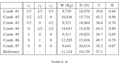
A total number of 36 optimizations have been run with the new method using a standard GA. The first ten of them have been used to calibrate the complexity function. The remaining 26 have been divided in two different campaigns. The first campaign consisted in seven combinations of the three weight factors. That campaign has been run twice, using the results in the first campaign as additional seeds for the second campaign. This allowed for searching new regions in the parameter space. Table I shows the values of the three ingredients for the optimized individuals (the reference values are also provided) and the associated fitness.
TABLE I
THE SEVEN COMBINATIONS CONSIDERED IN THE FIRST OPTIMIZATION CAMPAIGN AND THEIR ASSOCIATED VALUES OF THE WEIGHT,DRAG,
COMPLEXITY,AND FITNESS OF THE OPTIMIZED CONFIGURATIONS
²1 ²2 ²3 W (Kg) D (N) C Φ
Comb. #1 1/3 1/3 1/3 9,759 18,070 39.6 0.84 Comb. #2 1/2 1/2 0 10,836 15,734 45.2 0.90 Comb. #3 1/2 0 1/2 9,521 18,964 38.6 0.76 Comb. #4 0 1/2 1/2 14,651 15,636 44.4 0.80 Comb. #5 1 0 0 9,511 19,025 38.7 0.85 Comb. #6 0 1 0 12,205 15,016 49.7 0.79 Comb. #7 0 0 0 9,641 20,614 38.2 0.67 Reference - - - 11,124 19,129 57.1
-TABLE II
COUNTERPART OF TABLEIFOR THE TWELVE COMBINATIONS IN THE SECOND OPTIMIZATION CAMPAIGN
²1 ²2 ²3 W (Kg) D (N) C Φ
Comb. #1 0 1/3 2/3 10,510 17,937 39.5 0.77 Comb. #2 0 2/3 1/3 15,181 15,223 46.2 0.80 Comb. #3 1/3 0 2/3 9,520 18,963 38.6 0.73 Comb. #4 1/3 2/3 0 11,158 15,426 46.7 0.87 Comb. #5 2/3 1/3 0 9,713 18,064 39.6 0.89 Comb. #6 2/3 0 1/3 9,520 18,963 38.6 0.79 Comb. #7 1/6 1/6 2/3 9,520 18,963 38.6 0.76 Comb. #8 1/6 2/3 1/6 11,149 15,436 46.7 0.84 Comb. #9 2/3 1/6 1/6 9,520 18,963 38.6 0.85 Comb. #10 1/4 1/4 1/2 9,520 18,963 38.6 0.80 Comb. #11 1/4 1/2 1/4 10,376 16,377 42.7 0.85 Comb. #12 1/2 1/4 1/4 9,520 18,963 38.6 0.84 Reference - - - 11,124 19,129 57.1
-The second campaign consisted in 12 new GA runs (with 12 new combinations of the weight factors), which have been seeded with the best individuals of the first campaign. Results are presented in table II.
The performance of the surrogates is tested comparing (in table III) the results obtained in the first optimization campaign, combination #1 with those obtained with the conventional optimization tool, optimizing with the same GA. Note that the relative error is always below 3%. Results for the remaining combinations in both campaigns are com-pletely similar, except for the restriction on lateral stability, which shows larger error (up to 7%) in some cases. This larger relative errors are due to round off errors in the AVL calculations, which play a role when this restriction shows quite small values. In any event, those errors could be de-creased by both retaining more modes in the HOSVD (which also requires calculating a larger number of snapshots) and improving the precision of the AVL method.
[image:3.595.307.546.94.221.2]TABLE III
COMPARISON BETWEEN THE CONVENTIONAL AND REDUCED OPTIMIZATION TOOLS IN COMBINATION#1,FIRST OPTIMIZATION
CAMPAIGN
Restriction Reduced tool Full tool Error
Cmα -2.81 -2.84 1.1%
Cnβ 0.13 0.13 0.0%
Cmδ -1.63 -1.68 3.1%
Cnδ 0.133 0.135 1.5%
Clmax 1.51 1.55 2.6%
Clmin -1.24 -1.21 2.5%
Optimization function Reduced tool Full tool Error
Weight (Kg) 9,759 10,052 3.0%
Drag (N) 18,070 18,070 0.0%
Complexity 39.6 39.6 0.0%
Total fitness 2.51 2.53 0.8%
divided by a factor of 260. On the other hand, the new tool requires a previous AVL-calculation of the snapshots, which requires about 122.5 CPU hours. If we added that time to the optimization computational effort, the resulting time is 124.1 hours. This means that the time needed to run just one opti-mization is reduced by a factor of 3.6, which is small. But, as it happen in the illustration above, conceptual optimization usually requires a quite large number of additional optimiza-tions runs, which do not require recalculating the surrogates provided that the flight conditions remain unchanged. As the number of additional optimizations increases, the benefit of the new method increases, approaching the asymptotic reduction factor of 260. For instance, in the 36 optimizations runs performed above, the reduction factor was 81.7. It is also to be noted that the CPU time required by the conventional computational tool (608 CPU days) would make this tool impractical in this task, while its counterpart for the reduced tool (7 days) is quite reasonable.
V. CONCLUSION
A method has been presented for optimization based con-ceptual design in Aeronautics that is made up of two levels. A GA is used to optimize a target function, which includes var-ious multidisciplinary ingredients. The technical disciplines are modeled using surrogates, which are constructed using a combinations of HOSVD and one-dimensional interpolation. The computation of the surrogates requires running the original computational tools at some structured, discretized values of the design parameters. Each technical discipline needs to run the computational tool only for the parameters involved in the discipline. Thus, the advantages of the surrogate models become more evident as the number of free parameters increase. This is because the computational effort to CFD calculate the snapshots databases (necessary to construct each surrogate) increases exponentially with the database dimension.
The surrogates are much more computationally efficient than the conventional tool and can be defined as independent of the various modeling parameters that must be tuned in advance. Thus, tuning as well as optimization can be performed using the surrogate models. For instance, in the example considered in the article, the number of free design parameters was nine and five additional tunable parameters
(the three weight in the objective function and the parameters b and m appearing in the definition of complexity) were present. In practice, more design and tunable parameters are present.
The illustration method of section III is rather simplified, but the advantages of the method would be even clearer in more realistic conceptual design problem, which could include:
1) A larger number of free design parameters in the definition of the HTPs and the VTP, to account for, eg., torsion in the HTP and higher order corrections in the already considered geometric properties.
2) A more detailed model for the structure
3) A better modelization of viscous drag and stall, using a description of the boundary layer.
4) A multi-fidelity approach, in which various aerody-namic models are sequentially used, in the whole parametric spaces and in subregions near pre-optimized configurations.
5) A gradient like method can be combined with the GA to speed up convergence of the elite individuals. We expect that the method presented in this article, which is flexible enough to be combined with any specific optimiza-tion method, is a promising alternative to current approaches in conceptual design tasks, which must be completed within specific cost and time constrains.
APPENDIX
A. Purely geometrical ingredients
The HTP and the VTP geometries are first described in terms of various design parameters. The two fitness ingredients that only depend on the geometry, namely the complexity and the viscous drag, are then considered.
1) Parametrization of the geometry: Both HTPs are de-fined similarly, using ageneratrix, which provides the centers of the chord wise sections. The generatrix of the right HTP is given by
x=λ3y if y >0,
z=λ4y if 0< y < y1,
z=λ4y+λ5(y−y1)2 if y > y1,
(11)
where y1 = λ1/ p
1 +λ2
3+λ24. Here, x, y, and z are
the Cartesian coordinates in a system with origin at the center of the root section; the x axis is defined along the fuselage axis, the z axis is contained in the plane of the root section pointing upwards, and they axis perpendicular to the fuselage symmetry plane pointing to the right. Thus, the generatrix consists of a straight segment whose length isλ1, followed by a parabolic segment, whose length isλ2.
The HTPs are generated with NACA0012 profiles, with a chord distribution defined by the taper ratio,λ6; the airfoils
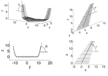
are contained in the normal plane of the projection of the generatrix on the y-z plane(see Fig. 2, left plots). The ruled surface generated by the mid lines of the HTP profiles will be referred to as the mid-lines surface.
The VTP geometry is simpler. Its planform is trapezoidal and the horizontal sections are NACA0012 profiles whose centers move along the VTPgeneratrix, which is defined as
Fig. 2. Generation of the HTPs
where 0 < z < λ7. The distribution chord is given by the
taper ratio, λ9.
2) Geometrical complexity: The complexity depends only on the geometry, and is defiend adding the contributions from the HTP and the VTPs, as
CEM P EN N AGE= (1 +b)(2CHT P+CV T P) (13)
where the penalty b is applied when the VTP is present (it can be absent in some configurations). The complexity of the HTP is estimated as
CHT P =
Z λ1+λ2
0
mp1 +κ(s)mds (14) wheresis the arch length along the generatrix and κis the curvature of the generatrix. Since the generatrix of the VTP is a straight line, it exhibits zero curvature and the complexity of the VTP is defined as
CV T P =
Z λ7√1+λ2 8
0
mp
1 +κ(s)mds=λ
7 q
1 +λ2 8 (15)
whereλ7 andλ8 are defined as above.
The exponent m and the penalty b are to be calibrated, nothing that increasing m emphasizes the effect of high concentrated values ofκ, which occur in, e.g., sharp junctions between smooth pieces of the HTP. After some calibration that consisted in a previous campaign of GA runs (for various values of m and b) similar to the campaigns described in section III, the following values have been selected
b= 0.1, m= 2 (16)
Since the calculation of the integrals appearing in (14) and (15) is computationally inexpensive, no surrogate model is constructed to calculate complexity.
3) Viscous drag: The total viscous drag is calculated at cruise conditions (altitude=15,000m, Mach=0.8) using a flat plate boundary layer analogy, which allows for adding the contributions of the HTPs and the VTP, as
D= 2DHT P +DV T P (17)
The contribution from each HTP (the VTP is treated simi-larly) is given by
DHT P =1
2cfρ∞U
2
∞WA (18)
whereρ∞ and U∞ are the density and velocity at the free
stream, WA is the wetted area of the HTP, and cf is the
friction coefficient. The latter is estimated as [11]
cf = 0.455/(logRem)2.588, (19)
whereRemis the Reynolds number, based on the HTP mean
chord.
As it happened with complexity, these calculations are computationally inexpensive and thus no surrogate model is constructed.
B. Purely aerodynamic restrictions
Aerodynamic restrictions involve the stall and the stability and control derivatives of the empennage. Aerodynamic interaction between HTP and VTP is neglected. Stability and control derivatives are calculated adding the contri-butions of the HTP and VTP, which are calculated using the AVL method to the fuselage/wings/HTP and the fuse-lage/wings/VTP, respectively.
1) Stability and control:AVL is run at zero angle of attack and zero sideslip angle, altitud=1,500m, and M=0.5. The derivatives of the vertical and lateral moments coefficientes with respect to the angle of attack αand the sideslip angle β provided by the AVL method, Cmα and Cnβ, are made
dimensionless with the dynamic pressure at the free stream, a wing reference area, and the mean chord of the wing. Thus the contributions of the HTP and VTP are re-scaled in the same way and they can be added to obtain the stability derivatives of the empennage. The control derivatives with respect to the deflection of the vertical control surface, δ, are defined similarly. Summarizing, the stability and control derivatives are defined as
CHT P
mα =F1(λ1, ..., λ6), CnβHT P =F2(λ1, ..., λ6) (20)
CV T P
nβ =F3(λ7, λ8, λ9) (21)
CHT P
mδ =F4(λ1, ..., λ6), CnδHT P =F5(λ1, ..., λ6) (22)
CnδV T P =F6(λ7, λ8, λ9) (23)
where functions F1, ..., F6 are treated using as surrogate
model that resulting from applying HOSVD+I to these functions.
2) Stall restrictions: The flight conditions to impose stall restrictions are: altitude=1,500m, Mach=0.2, andβ = 0. As explained in section III.B, imposing stall restrictions require to calculate with AVL the span-wise maximum (atα= 25◦)
and minimum (atα =−25◦) values of the chord-wise lift
coefficients on the various cross sections,ClmaxandClmin.
These are
Clmin=F7(λ1, ..., λ6), Clmax=F8(λ1, ..., λ6) (24)
As above, these two functions are treated using as surrogate model that resulting from applying HOSVD+I to these functions.
C. Aerodynamics + structures ingredients
Aerodynamic loads result from AVL calculations per-formed at Mach=0.5, altitud=1,500m, and three combina-tions of the angle of attack and the sideslip angle, namely
[image:5.595.51.273.57.214.2]Fig. 3. The structure
1) Aerodynamic loads: AVL provides the local pressure distribution p(x, s), where x is the stream-wise coordinate and s is the arch length along the generatrix. Using these, the shear force, bending moment, and torsional moment are calculated and a safety factor of 1.5 is applied. These calculation must be performed for all possible configurations of the HTP (namely, for all combinations of the HTP design parametersλ1, . . . , λ6), and the tree above mentioned
com-binations of the angle of attack and the sideslip angle. Since the two pieces of the HTP must be considered independently, a total number of six distributions of shear force,Q, bending moment, M, and torsional moment,T must be considered. These depend ons0 and the six free parameters of the HTP,
as
Q=Qj(λ1, ..., λ6, s0),
M =Mj(λ1, ..., λ6, s0),
T =Tj(λ1, ..., λ6, s0)
(25)
for j = 1, ...,6. The HOSVD+I method provides surrogates for these eighteen functions. The VTP is treated similarly but the load distributions are independent of the angle of attack, namely
Q=Q7(λ7, λ8, λ9, z0),
M =M7(λ7, λ8, λ9, z0),
T =T7(λ7, λ8, λ9, z0)
(26)
Again, the HOSVD+I methodology provides surrogates for these tree functions.
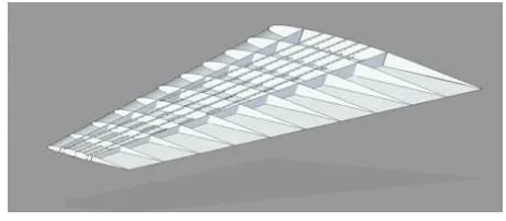
2) Weight: The weight is associated to the structure needed to support the loads calculated above. Concerning the HTP (the VTP is treated similarly), the main assumption is that aerodynamic loads are completely supported by a longitudinal torsion box, which extends span-wise along the HTP. The torsion box (Fig.3) is formed by a leading and a trailing spars, which are located at 20% and 55% of the chord, respectively, and the cover joining both spars on their upper and lower edges, to complete the box. The height and the width of the box vary spanwise and will be denoted as handd, respectively.
Thus, the structural elements in the torsion box are the cover and the spars, whose thicknesses are to be determined. Cover thickness includes the actual skin thickness plus the effects of stringers, and it is estimated setting up the admissible stress σadm = 360M P ain
tcov≈ M(s)
σadmd(s)h(s) (27)
wheres is the arch length along the generatrix of the HTP, as above, and M is provided by a surrogate, as explained above.
The spars thickness is defined as
tsp(s)≈qmax
τadm
(28)
where the admissible shear stress is set toτadm = 180M P a
and the maximum shear flow is calculated as
qmax(s) =
¯ ¯ ¯
¯2d(Ts()sh)(s) ¯ ¯ ¯ ¯+
¯ ¯ ¯ ¯2Qh((ss))
¯ ¯ ¯
¯ (29)
whereT and Q are obtained with surrogates, as explained above. A minimum thickness of 2.5mm is considered in both the cover and the spars.
Once the thickness of the critical case at each section is obtained. The weight is computed as
W = 2RS
T B
ρcovd(s)tcov(s)+ρsph(s)tsp(s)
c(s) dS
+ρS
³
AS−
R
ST B
d(s)
c(s)dA
´ (30)
where the first integral accounts for both the weight of the equivalent upper and lower panels of the box and the spars weight, and the third term accounts for the remaining of the stabilizer. In these integrals,ST Bis that part of the mid-lines
surface of the HTP occupied to the torsion box,AS is the
total area of the mid-lines surface, and thedA=sinϕdxds is the differential area along the mid-lines surface;ρcov and
ρsp are the skin and spars material density, respectively, and
ρs is the density per unit surface of the stabilizer part that
is not torsion box, defined in such a way that it accounts for the weight of other components and mechanical parts.
ACKNOWLEDGMENT
This research has been partially funded by the Spanish Ministry of Education, under Grants DPI2009-07591 and TRA2010-18054.
REFERENCES
[1] I. Kroo, S. Altus, R. Braun, P. Gage, and I. Sobieski, “Multidisci-plinary optimisatization methods for aircraft preliminary design,” 5th AIAA/USAF/NASA/ISSMO Symposium on Multidisciplinary Anal-ysis and Optimisation, Panama City, Florida, AIAA 94-4325, Tech. Rep., September 1994.
[2] N. E. Antoine and I. Kroo, “Aircraft optimization for minimal envi-ronmental impact,”Journal of Aircraft, vol. 41, no. 4, pp. 790–797, 2004.
[3] ——, “Framework for aircraft conceptual design and environmental performance studies,”AIAA Journal, vol. 43, no. 10, pp. 2100–2109, 2005.
[4] J. A. Nelder and R. Mead, “A simplex method for function minimiza-tion,”Computer journal, vol. 7, no. 4, pp. 308–313, 1965.
[5] G. Schumacher, I. Murra, L. Wang, A. Laxander, O. O’Leary, and M. Herold, “Multidisciplinary design optimisatization of a regional aircraft wing box,” 9th AIAA/ISSMO Multidisciplinary Analysis and Optimisation Conference, Atlanta, Georgia, Tech. Rep., September 2009.
[6] P. Piperni, M. Abdo, and F. Kafyeke, “The application of multi-disciplinary optimization technologies to the design of a business jet,” 10th AIAA/ISSMO Multidisciplinary Analysis and Optimisation Conference, Albany, New York, Tech. Rep., August 2004.
[7] N. V. Queipo, R. T. Haftka, W. Shyy, T. Goel, R. Vaidyanathan, and P. K. Tucker, “Surrogate-based analysis and optimization,”
Progr. Aerosp. Sci., vol. 41, no. 1, pp. 1–28, 2005.
[8] M. Price, S. Raghunathan, and R. Curran, “An integrated systems engineering approach to aircraft design,”Progr. Aerosp. Sci., vol. 42, no. 4, pp. 331–376, 2006.
[9] A. I. J. Forrester and A. Keane, “Recent advances in surrogate-based optimization,”Progr. Aerosp. Sci., vol. 45, no. 1, 2009.
[10] L. Lorente, J. M. Vega, and A. Velazquez, “Compression of aerodynamic databases using singular value decomposition,”
Aerosp. Sci. Tech., vol. 14, no. 3, pp. 168–177, 2010.
[image:6.595.44.275.53.154.2]