A Large Scale Pseudoword Based Evaluation Framework for State of the Art Word Sense Disambiguation

Evaluation Framework for State-of-the-Art

Word Sense Disambiguation

Mohammad Taher Pilehvar

Roberto Navigli

Sapienza University of Rome

The evaluation of several tasks in lexical semantics is often limited by the lack of large numbers of manual annotations, not only for training purposes, but also for testing purposes. Word Sense Disambiguation (WSD) is a case in point, as hand-labeled data sets are particularly hard and time-consuming to create. Consequently, evaluations tend to be performed on a small scale, which does not allow for in-depth analysis of the factors that determine a system’s performance.

In this article we address this issue by means of a realistic simulation of large-scale evalua-tion for the WSD task. We do this by providing two main contribuevalua-tions: First, we put forward two novel approaches to the wide-coverage generation of semantically aware pseudowords (i.e., artificial words capable of modeling real polysemous words); second, we leverage the most suitable type of pseudoword to create large pseudosense-annotated corpora, which enable a large-scale experimental framework for the comparison of state-of-the-art supervised and knowledge-based algorithms. Using this framework, we study the impact of supervision and knowledge on the two major disambiguation paradigms and perform an in-depth analysis of the factors which affect their performance.

1. Introduction

Word Sense Disambiguation (WSD) is a core research field in computational linguis-tics dealing with the automatic assignment of senses to words occurring in a given context (Navigli 2009, 2012). There are two major paradigms in WSD: supervised and knowledge-based. Supervised WSD starts from a training set and learns a computa-tional model of the word of interest, which is later used at test time to classify new instances of the same word. Knowledge-based WSD, instead, performs the disambigua-tion task by using an existing lexical knowledge base—that is, a semantic network to which graph algorithms, for example, can be applied. However, both disambiguation paradigms have to face the so-called knowledge acquisition bottleneck, namely, the

∗Department of Computer Science, Sapienza University of Rome, Viale Regina Elena 295, Roma 00161, Italy. E-mail:{pilehvar,navigli}@di.uniroma1.it.

Submission received: 31 August 2013; revised version received: 31 October 2013; accepted for publication: 6 March 2014.

difficulty of capturing knowledge in a computer-usable form (Buchanan and Wilkins 1993).

Unfortunately, providing knowledge on a large scale is a time-consuming process, which has to be carried out separately for each word sense and repeated for each new language of interest. Importantly, the largest manual efforts for providing a wide-coverage semantic network and training corpus for WSD date back to the early 1990s for the WordNet dictionary (Miller et al. 1990; Fellbaum 1998) and to 1993 for the SemCor corpus (Miller et al. 1993). In fact, although cheap and fast annotations could be obtained by means of the Amazon Mechanical Turk (Snow et al. 2008) or voluntary collaborative editing such as in Wikipedia (Mihalcea 2007), producing annotated resources manually is still an arduous and understandably infrequent endeavor. Despite recent efforts in this direction, including OntoNotes (Pradhan et al. 2007b) and MASC (Ide et al. 2010), most work is now aimed either at the automatic acquisition of training data (Zhong and Ng 2009; Moro et al. 2014) and lexical knowledge resources (Navigli 2005; Cuadros and Rigau 2008; Ponzetto and Navigli 2010), or at the large-scale acquisition of an-notations via games (Venhuizen et al. 2013) or even video games with a purpose, as recently proposed by Vannella et al. (2014). As a result, state-of-the-art performance can be achieved with both supervised (Zhong and Ng 2010) and knowledge-based (Navigli and Ponzetto 2012b; Moro, Raganato, and Navigli 2014) paradigms in different settings and conditions. Moreover, existing studies hypothesize that this performance can be further improved when larger amounts of manually crafted sense-tagged data or structured knowledge are made available (Martinez 2004; Cuadros and Rigau 2008; Martinez, de Lacalle, and Agirre 2008; Navigli and Lapata 2010). All these results, how-ever, are obtained on small-scale data sets with different characteristics, thus making it difficult to draw conclusions on the factors that impact the system’s performance.

In this article we address this issue by providing two main contributions:

r

artificial words that model real words by preserving their semantics as much as possible. Our semantically aware pseudowords can be used to model any word in the lexicon,1_{therefore aiming for wide coverage.}

We perform different experiments to show that our semantically aware pseudowords are good at modeling existing ambiguous words in terms of disambiguation difficulty, representativeness, and distinguishability of the artificial senses.

r

time, a large-scale evaluation framework for WSD. Using this framework, we are able to perform an experimental comparison of state-of-the-art systems for supervised and knowledge-based WSD on a very large data set made up of millions of sense-tagged sentences. Our large-scale framework enables us to carry out an in-depth analysis of the factors and conditions that determine the systems’ performance.

In our recent work (Pilehvar and Navigli 2013), we presented an approach for the generation of semantically aware pseudowords, called similarity-based pseudowords. At the core of this approach was the Personalized PageRank algorithm (Haveliwala

2002) on the WordNet graph, which was utilized to find the most semantically similar monosemous representative for a given sense of a real ambiguous word. The main strength of the similarity-based approach lies in its flexibility, allowing high minimum frequency constraints to be set on its selection of pseudosenses, while maintaining its overall sense modeling quality.

In this article we extend our previous work as follows: 1) we propose a new approach for generating semantically aware pseudowords which leverages topic signa-tures; 2) we utilize the best type of pseudoword to create a novel framework for large-scale evaluation and comparison of WSD systems; 3) based on this framework, we carry out a large-scale comparison of state-of-the-art supervised and knowledge-based WSD algorithms; and 4) we study the impact of the amount of supervision and knowledge on the two major disambiguation paradigms and perform an in-depth analysis of the factors and conditions that determine their performance.

The remainder of this article is organized as follows: In Section 2 we survey related work concerning the impact of the knowledge acquisition bottleneck on WSD and pro-vide an explanation of our pseudoword-based approach. In Section 3 we describe pseu-dowords and overview the existing approaches to their generation. We then present two new approaches that address the issues associated with existing pseudowords, hence enabling the wide-coverage generation of semantically aware pseudowords. In Sec-tion 4, we perform various experiments to assess the degree of realism of our proposed pseudowords. We then illustrate how we leverage our pseudowords to generate large sense-tagged data sets in Section 5. The experimental set-up for pseudoword-based WSD is described in Section 6. Experimental results as well as the findings are presented and discussed in Section 7. Finally, we provide concluding remarks in Section 8.

2. Related Work

2.1 Supervised WSD and the Knowledge Acquisition Bottleneck

Over the last few decades, WSD systems have been suffering from disappointingly low performance, especially in an all-words setting in which one has to cover the entire lexicon of the given language (Snyder and Palmer 2004; Pradhan et al. 2007a). In fact, one of the major obstacles to high-performance WSD is the so-called knowledge acquisition bottleneck (Gale, Church, and Yarowsky 1992b): In order to learn accurate word experts, supervised systems need training data for each word of interest, a very demanding task as far as wide coverage is concerned (i.e., one which would require the manual annotation of millions of word instances in context).

An alternative approach to acquiring sense-tagged data is to leverage multilingual resources such as parallel corpora (Chan and Ng 2005a; Wang and Carroll 2005; Chan, Ng, and Zhong 2007). Most of these techniques, however, require human intervention for mapping the translation of a word in the target language to the correct sense of the corresponding word in the source language. Recently, Zhong and Ng (2009) tackled this problem by using a bilingual dictionary. However, the dictionary has to be aligned to the sense inventory of interest (e.g., WordNet) and a large parallel corpus must be available that covers the full range of meanings in a lexicon. The approach, implemented in a system based on Support Vector Machines and called It Makes Sense (Zhong and Ng 2010, IMS), attains state-of-the-art performance on lexical sample and all-words WSD tasks. However, according to our calculation on the available models,2_{this approach can}

only provide training examples for about one third of ambiguous nouns in WordNet, more than half of which have only one of their senses covered.

Middle-ground approaches have also been proposed that either mix arbitrary sense-tagged corpora with a small amount of sense-tagged data for the domain of interest (Khapra et al. 2010), or estimate the sense distribution of the new domain data set with the help of parallel corpora (Chan and Ng 2005b, 2007), thus relieving the knowledge acquisi-tion bottleneck. However, domain adaptaacquisi-tion approaches typically suffer from lower disambiguation performance and still require annotated data for the domain of interest.

2.2 Knowledge-Based WSD and the Knowledge Acquisition Bottleneck

Knowledge-based WSD systems are equally affected by the knowledge acquisition bottleneck, as they exploit the knowledge and structure of lexical knowledge bases in carrying out the disambiguation task. Therefore, in order to obtain high performance, knowledge-based systems are applied to large, wide-coverage lexical knowledge bases. However, the largest hand-crafted resource of this kind (i.e., WordNet) dates back to 1990 with subsequent updates, which attests to the high cost of knowledge engineering on a large scale. Moreover, WordNet mostly provides taxonomic knowledge, while ne-glecting much syntagmatic relational information between concepts. As a consequence, over the past few years several automatic techniques have been proposed that enrich WordNet with new relation edges, such as those obtained from disambiguated glosses (Mihalcea and Moldovan 2001), collocation dictionaries (Navigli 2005), topic signa-tures (Agirre et al. 2001; Cuadros and Rigau 2008), and collaborative semi-structured resources (Hovy, Navigli, and Ponzetto 2013).

Enriched knowledge bases have been shown to greatly benefit graph-based ap-proaches such as Personalized PageRank (PPR; Agirre, de Lacalle, and Soroa 2009; Agirre, Lopez de Lacalle, and Soroa 2014), context-based vertex degree (Navigli and Lapata 2010), or, more recently, a densest-subgraph algorithm that jointly performs WSD and Entity Linking (Moro, Raganato, and Navigli 2014). Not only do these methods outperform supervised WSD systems when applied within a domain, but, when the knowledge base is enriched with tens of thousands of semantic relations automatically extracted from Wikipedia, performance comparable to that of state-of-the-art supervised systems can be obtained in a general all-words setting, too (Ponzetto and Navigli 2010; Moro, Raganato, and Navigli 2014).

Recently, a multilingual graph-based WSD approach has been developed that lever-ages a large multilingual semantic network, called BabelNet (Navigli and Ponzetto

2012a), to achieve state-of-the-art results on both general all-words and domain-oriented WSD (Navigli and Ponzetto 2012b). Experimental results show that the joint use of multilingual knowledge enables further improvements over monolingual WSD. However, the power of this disambiguation system lies mainly in its usage of the BabelNet multilingual semantic network. In fact, Agirre, Lopez de Lacalle, and Soroa (2014) showed that under similar conditions (i.e., when the same lexical knowledge base was used), the PPR algorithm can outperform the graph-based WSD algorithms used by Navigli and Ponzetto (2012b).

2.3 The Supervision vs. Knowledge Dilemma

Unfortunately, as of today we do not have unequivocal insights into which disambigua-tion paradigm is more suitable under which condidisambigua-tions. As a matter of fact, not only does each implemented system come with its own amount and kind of supervision or knowledge, making it hard to determine the contribution of the supervision or knowl-edge vs. that of the WSD algorithm, but test data sets are small, typically comprising one or two thousand sense-tagged word items, which prevents us from drawing solid conclusions. Even the largest annotation effort ever—namely, the SemCor sense-tagged data set (Miller et al. 1993), comprising around 235,000 semantic annotations—covers only about 15% of word types in WordNet with an average of 10 instances per word, thus precluding large-scale experimental studies.

A possible solution to this current limit in the evaluation of WSD systems is to generate sense-annotated data with the help of artificial ambiguous words, called pseudowords. Pseudowords are created by conflating a set of unambiguous words called pseudosenses. The idea of pseudowords was simultaneously introduced by Gale, Church, and Yarowsky (1992a) and Sch ¨utze (1992) as a means of generating large amounts of artificially sense-tagged evaluation data for WSD algorithms. Pseudowords have also been used in other work aimed at studying the effects of data size on machine learning for confusion set disambiguation (Banko and Brill 2001), evaluation of selec-tional preferences (Erk 2007; Bergsma, Lin, and Goebel 2008; Chambers and Jurafsky 2010), or Word Sense Induction (Di Marco and Navigli 2013; Jurgens and Stevens 2011). However, constructing a pseudoword by merely combining a random set of unam-biguous words picked out to be in the same range of occurrence frequency (Sch ¨utze 1992), or leveraging homophones and OCR ambiguities (Yarowsky 1993), does not provide a suitable model of a real polysemous word (Gaustad 2001), since in the real world different senses, unless homonymous, share some semantic or pragmatic relation. For this reason, random pseudowords, when used for WSD evaluation, were found to be easier to disambiguate compared with the human-generated pseudowords (Gaustad 2001), thus leading to an optimistic upper-bound estimate on the performance of WSD classifiers (Nakov and Hearst 2003).

Several researchers addressed the issue of producing pseudowords that can model semantic relationships between senses. To this end Nakov and Hearst (2003) used lexical category membership from a medical term hierarchy (extracted from MeSH3[Medical Subject Headings]) to create “more plausible” pseudowords. By considering the distri-butions from lexical category co-occurrence, they produced a set of pseudowords that were closer to real ambiguous words in terms of disambiguation difficulty than random

pseudowords. However, this approach requires a specific hierarchical lexicon and falls short of creating many pseudowords with high polysemy.

More recent work has focused on the identification of monosemous representatives in the surroundings of a sense, that is, selected among concepts directly related to the given sense. Senses of a real ambiguous word have been modeled by picking out the most similar monosemous morpheme from a Chinese hierarchical lexicon (Lu et al. 2006). Pseudowords are then constructed by conflating these morphemes accordingly. However, this method leverages a specific Chinese hierarchical lexicon, in which differ-ent levels of the hierarchy correspond to differdiffer-ent levels of sense granularity. A more flexible approach is proposed by Otrusina and Smrz (2010), who model ambiguous words in WordNet. For each particular sense, they search its surroundings in the Word-Net graph in order to find an unambiguous representative for that sense.

Unfortunately, as we discuss in detail in the next section, none of these proposals can enable a large-scale evaluation framework for WSD, mainly because they suf-fer from coverage issues that prevent the creation of wide-coverage sense-annotated data sets. In this article we propose new pseudoword generation techniques that allow for the creation of thousands of artificial words having sufficient occurrence coverage within a large corpus. We then leverage our semantically aware pseudowords to create an evaluation framework which enables a large-scale comparison of state-of-the-art supervised and knowledge-based WSD.

3. Pseudowords

Apseudowordis an artificially created ambiguous word created by concatenating two or more distinct words. Formally, p=w1*w2*. . . *wn is a pseudoword with polysemy degreenwhere eachwiis called apseudosense. Each pseudosense is usually identified by an unambiguous word drawn from the set of monosemous words in a given lexicon (e.g., WordNet). For instance,press release*ship*camelis a pseudoword with three distinct meanings explicitly identified by its pseudosenses (i.e.,press release,ship, andcamel).

Pseudowords are particularly useful for creating artificially annotated data sets. To this end, an untagged corpus C is automatically annotated with a pseudoword

p=w1*w2*. . . *wnby substituting all occurrences ofwiinCwithpfor each pseudosense i∈ {1,. . .,n}. As an example, consider the following three sentences:

a1. The goal of apress releaseis to attract favorable media attention.

a2. For ashipto float, its weight must be less than that of the water displaced by its hull.

a3. During the winter, thecamelcan go fifty days without being watered.

In order to generate annotated data, it is enough to replace the individual occur-rences ofpress release,shipandcamelwith the pseudowordpress release*ship*camel, while noting the replaced term as the corresponding sense:

b1. The goal of apress release*ship*camel_{press release}is to attract favorable media attention.

b2. For a press release*ship*camel_ship to float, its weight must be less than that of the water

displaced by the hull.

b3. During the winter, thepress release*ship*camel_camelcan go fifty days without being watered.

be unambiguous, so as to avoid the introduction of uncontrolled ambiguity. Another constraint is that the pseudosensewimust appear in a sufficient number of sentences in the corpusC. This constraint on the occurrence frequency guarantees that there exist as many sentences in the corpus as the number of annotated sentences that are requested for the task of interest which will exploit the resulting annotated corpus.

The pseudoword in our example was generated by randomly selecting three monosemous words from WordNet. This can be considered as the most immediate approach for generating a pseudoword where constituents are randomly picked from the set of all monosemous words given by a lexicon. This results in a set of pseudowords (hereafter called random pseudowords) that are highly likely to have semantically unrelated pseudosenses. However, we know that the different senses of a real word are often in a semantic or etymological relationship. Therefore, random pseudowords can only model homonymous distinctions (such as thecentimeter vs.curiumsenses of the noun cm), and fall short of modeling systematic polysemy (such as the lack vs.

insufficiencysenses of the noundeficiency).

A pseudoword generation approach ought to be able to address this weakness of random pseudowords. A possible solution is to create pseudowords that model existing ambiguous words by providing, for each pseudoword, a one-to-one correspondence be-tween each pseudosense and a corresponding sense of the modeled word. For instance,

lack*shortfallis a good pseudoword modeling the real worddeficiencyas its pseudosenses preserve the meanings of their corresponding real word’s senses. We call artificial words of this kindsemantically aware pseudowords, in that they aim at listing senses that are in specific relations to each other, thus mirroring the relations existing between the senses of real words in the lexicon. For example, the lack-insufficiency relation is encoded in the pseudoword fordeficiency, which would not be possible if we generated a random pseudoword.

Semantically aware pseudowords enable the generation of artificially annotated data sets that have similar properties to their real counterparts and this makes them particularly suitable for the evaluation of WSD and Induction algorithms (Bordag 2006; Jurgens and Stevens 2011; Di Marco and Navigli 2013). In fact, in a real sense-annotated data set different senses of a word appear in distinct contexts. The extent of this dis-tinction, however, depends on the semantic relatedness of the corresponding senses. The intuition behind semantically aware pseudowords is that they model each sense of an ambiguous word through a semantically similar monosemous representative that should appear naturally in contexts that are similar to those of its corresponding real sense. For this reason, these pseudowords should be expected to result in data sets wherein the distinctions between different sense contexts are similar to those in real sense-annotated data sets.

In the next three sections we describe three techniques, two of which are presented in full detail for the first time in this article, for the generation of semantically aware pseudowords that use WordNet as the reference lexicon. In what follows we focus on nominal pseudowords, and leave the extension to other parts of speech to future work.

3.1 Vicinity-Based Pseudowords

representatives were selected among monosemous relatives (i.e., unambiguous words that are structurally related to a given sense). This method for finding monosemous representatives for senses has been in use since 1998, when it was first proposed for the unsupervised acquisition of sense-tagged corpora (Leacock, Chodorow, and Miller 1998).

Specifically, Otrusina and Smrz (2010) exploit WordNet, whose conceptual units are synonym sets, called synsets, which encode the different meanings of words. In order to find a monosemous representative for a given synset, the approach (hereafter referred to as the vicinity-basedapproach) performs a search on the set of words in the same synset and the surrounding ones (i.e., the synsets connected to that synset by means of WordNet’s lexico-semantic relations). These related synsets include siblings and direct hyponyms. In the case where no monosemous candidate could be found among these synsets, the search space is further extended to hypernyms and meronyms.

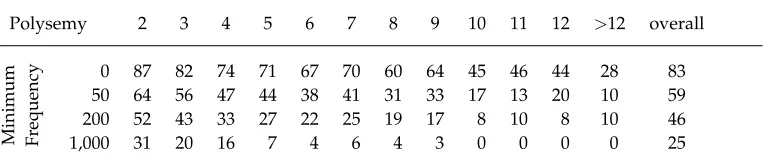
As an example, consider the ambiguous nouncoke, which has three senses (i.e., fuel, drink, and drug) in WordNet 3.0. We show in Table 1, for each of the three senses of coke, the set of nouns in the corresponding synset as well as in the surrounding synsets. Monosemous words are shown in bold in the table. As can be seen, there exist multiple monosemous candidates for each sense (coca cola, pepsi, and pepsi cola

for the second sense;nose candy,cocaine, andcocainfor the third sense; and dozens of candidates in the direct siblings’ vicinity of the first sense). Among these candidates Otrusina and Smrz (2010) select those whose occurrence frequency ratio in a given text corpus is most similar to that of the senses of the corresponding real word as given by a sense-annotated corpus. However, calculating the occurrence frequency of individual senses of a word requires a large-enough sense-tagged corpus. This dependency on sense-annotated data is a disadvantage of the vicinity-based approach that limits its ability in modeling arbitrary words.

Table 1

Synset neighbors of the three senses ofcoke(We use the sense notation of Navigli [2009] where

theith_{sense of wordwis denoted asw}i_{. We also highlight monosemous words in bold.)}

Synset literals sense 1 {coke1}

sense 2 {coca cola1_{, coke}2_}

sense 3 {coke3_{, blow}6_{,nose candy}1_{, snow}4_{, C}12_}

Direct siblings sense 1 {biomass1_{}, {butane}1_{}, {charcoal}1_{, wood coal}2_{}, {coal gas}1_},

{coke1}, {diesel oil1}, diesel fuel1}, {fire7}, {fossil fuel1},

{fuel oil1_{, heating oil}1_{}, {gasohol}1_{}, {gasoline}1_{, gasolene}1_, gas3_,petrol1_{},{illuminant}1_},{kerosene1_,kerosine1_{,lamp oil}1_, coal oil1}, {methyl alcohol1, wood alcohol1, wood spirit1},

{nuclear fuel1_{}, {propane}1_{}, {red fire}1_{}, {combustible}1_, combustible material1_{}, {water gas}1_{}, {firewood}1_{}, {igniter}1_,

ignitor1_{, lighter}1_}

sense 2 {Pepsi1_{,pepsi cola}1_}

sense 3 {basuco1_},{crack8_{, crack cocaine}1_{, tornado}2_}

Hypernyms sense 1 {fuel1_}

sense 2 {cola2_{, dope}3_}

sense 3 {cocaine1_,cocain1_}

Hyponyms sense 1

-sense 2

-Table 2

Noun coverage percentage of vicinity-based pseudowords by degree of polysemy for different values of minimum frequency.

Polysemy 2 3 4 5 6 7 8 9 10 11 12 >12 overall

Minimum Frequency

0 87 82 74 71 67 70 60 64 45 46 44 28 83

50 64 56 47 44 38 41 31 33 17 13 20 10 59

200 52 43 33 27 22 25 19 17 8 10 8 10 46

1,000 31 20 16 7 4 6 4 3 0 0 0 0 25

In addition to this limitation, the vicinity-based approach suffers from lack of flexibility in generating pseudowords that can be leveraged for creating a large-scale pseudosense-tagged corpus, where we need each pseudosense to occur with a relatively large minimum frequency. Due to its small search space, the approach falls short of identifying suitable monosemous representatives for many given senses, which under-mines its ability to cover most of the ambiguous nouns in WordNet. We show in Table 2 the percentage of nouns in WordNet that could be modeled using the vicinity-based approach when Gigaword (Graff and Cieri 2003) was used as our corpus. Coverage statistics are presented for four different values of minimum frequency: 0 (no minimum frequency constraint), 50, 200, and 1,000. Besides the overall coverage (rightmost col-umn), in the table we also present the coverage percentage by degree of polysemy. Here, an ambiguous noun in WordNet is considered as covered by its corresponding vicinity-based pseudoword if, for each of its senses, a suitable monosemous candidate can be found in its surrounding that also satisfies the specified minimum frequency in the corpus. As can be seen from the table, the approach can only model about 60% of ambiguous nouns in WordNet 3.0 when a small minimum frequency of 50 sentences in the large Gigaword corpus is assumed. The coverage continues to drop with the increase of minimum frequency up to only 25% of the ambiguous nouns covered when a minimum frequency of 1,000 noun occurrences is required (last row of Table 2), with most of the covered words having low polysemy. This shows that the approach is not flexible enough for generating pseudowords that can be leveraged for creating large, wide-coverage pseudosense-annotated data sets.

In order to address the aforementioned coverage issue of the vicinity-based ap-proach, in the next two sections we propose two new approaches for the generation of semantically aware pseudowords.

3.2 Similarity-Based Pseudowords

This expands the search space for finding pseudosenses from a small set of surrounding synsets to virtually all synsets in WordNet.

In order to measure semantic similarity we used the PPR (Haveliwala 2002) algo-rithm, a graph-based technique that has been used previously as a core component for semantic similarity (Hughes and Ramage 2007; Pilehvar, Jurgens, and Navigli 2013) and WSD (Agirre and Soroa 2009; Agirre, Lopez de Lacalle, and Soroa 2014). PPR can be used to estimate a probability distribution denoting the structural importance of all the nodes in a graph for a given target node. When applied on a semantic network, such as the WordNet graph whose nodes are synsets and edges the lexico-semantic relations, the notion of importance can be interpreted as semantic similarity. The reason behind our selecting a graph-based similarity measure was that the alternative context-based methods, such as Lin’s (1998) measure, have been shown to require a wide-coverage sense-tagged data set in order to calculate similarities on a sense-by-sense basis for all words in the lexicon (Otrusina and Smrz 2010). Also, among WordNet-based approaches, PPR reports state-of-the-art results on semantic similarity (Agirre et al. 2009) and WSD data sets (Agirre, Lopez de Lacalle, and Soroa 2014), thus representing a suitable graph-based measure for finding the most appropriate pseudosenses.

In Algorithm 1 we present the procedure for the generation of our similarity-based pseudowords. The algorithm takes as input an ambiguous wordw, and generates its corresponding similarity-based pseudowordPw whoseith pseudosense models theith sense of w. Additionally, the algorithm provides, for each generated pseudoword, a confidence degree denoting the average ranking of the selected pseudosenses.

The algorithm models a given ambiguous word w by iterating over the synsets corresponding to its individual senses (lines 5–18) and identifying the most suitable monosemous representative for each. For each sense ofw, we run the PPR algorithm

Algorithm 1:Generate a similarity-based pseudoword

Input: an ambiguous wordwin WordNet

Output: asimilarity-basedpseudowordPwand a confidence scoreaverageRank

1 begin

2 P_w← ∅

3 totalRank←0

4 i←1

5 foreachs∈Synsets(w)do

6 similarSynsets←PersonalizedPageRank(s)

7 sortsimilarSynsetsin descending order;

8 foreachs0∈similarSynsetsdo

9 totalRank←totalRank+1

10 foreachw0∈SynsetLiterals(s0)do

11 if|Synsets(w0)|=1andFreq(w0)≥minFreqand@j :(j,w0)∈Pwthen

12 Pw←Pw∪ {(i,w0)}

13 go toline 17

14 end

15 end

16 end

17 i←i+1

18 end

19 averageRank←totalRank/|Synsets(w)|

Table 3

Top five entries of thesimilarSynsetslist for different senses of wordcoke(we show both

WordNet 3.0 offsets and synsets). The highest-ranking monosemous noun in each list is shown in bold.

Sense no. Offset PPR score Terms in synset (literals)

1

14685768-n 0.225 coke1

14875077-n 0.148 fuel1

00498836-v 0.096 coke4

00146138-v 0.038 change state1_{, turn}14

15100644-n 0.011 firewood1

2

07927931-n 0.237 cola2_{, dope}3

07928696-n 0.217 coca cola1, coke2

07927197-n 0.083 soft drink1

12197601-n 0.045 cola nut1_{, kola nut}1

07928790-n 0.040 pepsi1_{, pepsi cola}1

3

03060294-n 0.278 cocaine1_,cocain1

03066743-n 0.205 blow6_{, c}12_{, coke}3_{, nose candy}1_{, snow}4

03492717-n 0.046 hard drug1

00021679-v 0.041 cocainise1_{, cocainize}1

03060074-n 0.041 coca3

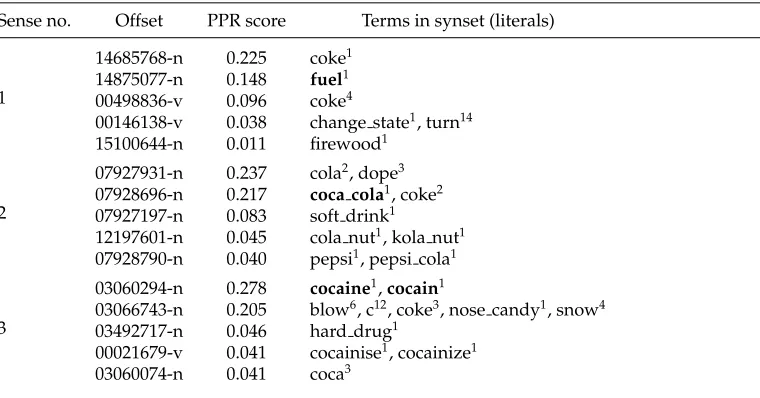
by initializing it from the corresponding synsets (line 6). As a result, PPR outputs a probability distribution over all synsets in WordNet denoting the semantic similarity of each synset tos.4_{The synset distribution is then sorted according to its values (line 7).}

We then go through all its nominal synsets (s0) in the search for a suitable monosemous noun (line 11). This search continues until a suitable candidate is found that satisfies the minimum occurrence frequencyminFreq. Upon finding this candidate, the selected monosemous wordw0is added as the corresponding pseudosense for theithsense ofPw (line 12). These steps are repeated for every sense ofw.

The higher the position of a selected pseudosense in the sorted list ofsimilarSynsets, the more confidence we have in the preservation of meaning. Therefore, we calculate a confidence score (averageRankin the algorithm) as the average of the synset’s positions (in the varioussimilarSynsetslists) from which the pseudosenses ofPw are picked out (line 19). We will later use this confidence score for evaluating our pseudowords. The algorithm returns as its output, for a given wordw, the corresponding pseudowordPw along with itsaverageRankscore (line 20).

Consider the generation process of the similarity-based pseudoword for our word

coke. Table 3 shows the list of top-five most similar synsets for each of the three senses of this term, as given by the PPR algorithm. Our algorithm selects the highest ranking monosemous candidates that satisfy the minimum frequency (=1,000 in the example) for each sense (shown in bold in the table). Hence,fuel*coca cola*cocaineis returned as the pseudoword corresponding to the wordcoke. Note that the top-ranking synsets are those also found by the vicinity-based approach. However, thanks to PPR working on the entire network, our similarity-based approach can back off to more distant,

Table 4

Sample similarity-based pseudowords generated (with minimum frequency of 1,000 occurrences in Gigaword) for four different nouns in WordNet 3.0. Words shown in bold are those that could not be modeled using the vicinity-based approach for the given minimum frequency. Pseudosenses which are not picked out from the surrounding of the corresponding sense (hence, could not be modeled using the vicinity-based approach) are shown in bold in the second column of the table.

word similarity-based pseudoword

bernoulli physicist*mathematician*astronomer

coach football coach*tutor*passenger car*clarence*public transport

green greenery*central park*labor leader*green party*river*golf course*greens*max

sunray sunbeam*vine*sunlight

though similar, synsets. We show in Table 4 some examples of ambiguous words along with their generated similarity-based pseudowords (minimum frequency is again set to 1,000).

Having the large search space of virtually all synsets in WordNet, the similarity-based approach is able to select a monosemous candidate for each sense from a relatively-large ranked list of similar synsets. This solves both the coverage and flex-ibility issues of the vicinity-based approach for higher values of minimum frequency. However, as mentioned earlier, the higher the position of a selected pseudosense in the sorted list ofsimilarSynsets, the more confidence we have in the preservation of meaning. For this reason, we analyzed theaverageRankvalues output by Algorithm 1 in order to see how often our algorithm needs to resort to lower-ranking items in thesimilarSynsets

list. We present in Table 5, for each polysemy degree and for six different values of

minFreq, the mean and mode statistics of the averageRank scores of all the generated pseudowords for all the nouns (up to polysemy degree 12) in WordNet. As can be seen in the table, the higher the value ofminFreq, the further the algorithm descends through

Table 5

Statistics ofaverageRankscores of similarity-based pseudowords: we show mean and mode

positions for six different values of minimum occurrence frequency (0, 200, 500, 1,000, 2,000, and 5,000) and for each polysemy degree (we show the average value in the case of multiple modes).

minFreq 0 200 500 1,000 2,000 5,000

poly. mean mode mean mode mean mode mean mode mean mode mean mode

2 2.0 1.0 10.7 2.0 16.9 2.0 28.3 4.0 52.2 3.0 66.8 3.5

3 2.2 2.0 9.7 2.0 15.4 4.7 23.4 4.7 39.6 6.3 51.6 11.7

4 2.3 2.0 8.6 3.0 14.2 7.8 22.5 10.9 33.4 12.3 45.9 18.3

5 2.2 2.0 8.5 5.0 14.6 5.6 21.9 16.0 33.7 14.4 48.3 18.2

6 2.3 2.0 9.0 4.0 15.6 3.8 21.3 12.2 26.5 17.2 41.2 26.0

7 2.2 2.0 8.0 6.0 13.0 8.4 17.8 7.7 26.0 18.9 40.7 27.3

8 2.2 2.0 8.5 4.0 12.7 9.8 19.4 16.1 29.8 28.7 44.1 42.6

9 2.2 2.0 7.5 4.0 12.3 12.4 17.5 17.6 26.4 30.2 40.9 37.9

10 2.2 2.0 7.1 5.0 11.5 7.9 16.2 15.0 25.6 19.2 38.1 38.1

11 2.4 2.0 7.7 8.0 12.0 15.3 16.5 11.5 23.9 7.5 37.9 35.7

12 2.4 2.0 7.7 4.0 12.9 12.9 17.5 23.3 25.7 25.7 44.2 32.5

>12 2.5 1.0 7.2 2.0 10.8 2.0 16.0 4.0 22.4 4.0 39.1 4.0

Table 6

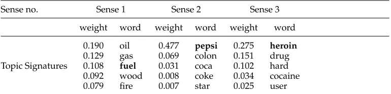
Top five words in the topic signatures for different senses of nouncoke. The first monosemous

noun for each sense is shown in bold.

Sense no. Sense 1 Sense 2 Sense 3

weight word weight word weight word

0.190 oil 0.477 pepsi 0.275 heroin

0.129 gas 0.069 colon 0.151 drug

Topic Signatures 0.108 fuel 0.031 coca 0.102 hard

0.092 wood 0.008 coke 0.034 cocaine

0.079 fire 0.007 star 0.025 user

the listsimilarSynsetsto select a pseudosense. However, the mode statistics in the table suggests that even whenminFreqis set to a large value, most of the pseudosenses are picked out from the highest-ranking positions in thesimilarSynsetslist.

3.3 Topic Signature-Based Pseudowords

As an alternative means of finding suitable monosemous representatives for word senses with the PPR algorithm, we propose using automatically generated topic signa-tures.Topic signatures(TS) are weighted topical vectors that are associated with senses or concepts (Lin and Hovy 2000). The dimensions of these vectors are the words in the vocabulary and their weights determine the relatedness of each of these words to the target word sense. These vectors can be obtained automatically from large corpora or the Web with the help of monosemous relatives.

In order to generate a TS-based pseudoword for a wordw, we first sort the weighted vectors associated with the senses ofw. Then, from each of these vectors, we select the monosemous word with highest relatedness (i.e., largest weight) which satisfies the minimum frequency constraint. The generation process of the TS-based pseudowords is very similar to that of similarity-based pseudowords: Whereas the latter performs a search in the sorted PPR vector of a particular sense to obtain a suitable monosemous representative, the former considers the sorted TS vector as its search space. Also note that the PPR vectors are indexed with synsets, whereas topic signatures have lemmas as their indices.

In our experiments we used the topic signatures provided by Agirre and de Lacalle (2004) for nominal senses of polysemous nouns in WordNet 1.6.5 The monosemous relatives for each sense were obtained by taking into account WordNet relations such as synonyms, hypernyms, hyponyms, and siblings that were later used to query the Web and create a large corpus. This corpus was then used to build topic signatures.

Table 6 shows the top five words in the topic signatures for different senses of the word coke. The first monosemous candidate for each sense is shown in bold (again, the minimum frequency is assumed to be 1,000 here). The corresponding pseudoword generated using this approach isfuel*pepsi*heroin.

Even though the TS-based approach shares the monosemous relatives idea with the vicinity-based approach, the additional step of gathering related instances for these representatives guarantees wider coverage. We calculated the coverage of TS-based

pseudowords to be 84% (over ambiguous nouns of WordNet 1.6 and with no minimum frequency constraint), which is comparable to that of vicinity-based pseudowords (i.e., 83%, see Table 2). We observed in Table 2 that the coverage of the vicinity-based pseudowords drops rapidly with the increase in minimum frequency such that for a minimum frequency of 1,000 only 25% of the polysemous nouns could be modeled. The TS-based approach, instead, provides a better flexibility for higher values of minimum frequency, hence enabling the generation of large-scale annotated data sets. Thanks to its larger search space, the TS-based approach is able to retain the same 84% coverage for a minimum frequency of 1,000.

Compared with the similarity-based pseudoword generation (described in Sec-tion 3.2), this approach provides a different way of overcoming the coverage issue of vicinity-based pseudowords. However, the former guarantees 100% coverage, whereas the latter suffers from the lack of monosemous relatives for a portion of WordNet senses, leading to non-optimal coverage.

4. Pseudoword Evaluation

In Sections 3.2 and 3.3 we presented two techniques for the generation of semantically aware pseudowords that were able to address the coverage and flexibility issues of the vicinity-based approach. In order to verify the ability of these pseudowords to model various properties of real ambiguous words, we performed three separate evaluations so as to assess them from different perspectives:

r

extrinsically study the impact of the pseudoword quality on the disambiguation performance (Section 4.1).

r

closeness of pseudosenses to their corresponding real senses (Section 4.2).

r

pseudosenses are specific to a fine-grained real sense rather than covering multiple senses (Section 4.3).

Given that our aim was to leverage these pseudowords for creating large-scale pseudosense-annotated data sets, we performed evaluations on pseudowords gener-ated with minFreqper pseudosense set to a high value of 1,000 (i.e., we can generate 1,000 annotated sentences for each pseudosense) using the English Gigaword corpus (Graff and Cieri 2003).

4.1 Disambiguation Difficulty of Pseudowords

of semantic similarity between pseudosenses as that of its corresponding real word, and therefore to exhibit a comparable degree of disambiguation difficulty to that of its corresponding real word.

We performed this evaluation in the style of earlier work (Otrusina and Smrz 2010; Lu et al. 2006). In order to test a pseudoword generation approach using this style, first, all the sense-tagged words in a manually annotated lexical sample data set are modeled using the approach. Next, a corresponding pseudosense-annotated data set is automatically constructed by sampling sentences from a corpus while maintaining the same number of training and test sentences for each word as that of the original manually tagged data set. A correlation analysis is then carried out to compare the disambiguation performance of a supervised WSD system on a given ambiguous word against its corresponding pseudoword. In this experiment we evaluate our similarity-based, TS-similarity-based, and, as baseline, random pseudowords. Owing to the fact that for the given minimum frequency of 1,000 we could generate only 5 of the 20 nouns using the vicinity-based approach, we had to exclude the approach from this experiment.

We selected the Senseval-3 English lexical sample data set (Mihalcea, Chklovski, and Kilgarriff 2004) as our manually sense-tagged corpus. The data set provides for 20 nouns of polysemy 3 to 10 an average number of 180 and 90 sense-tagged sentences in its training and test sets, respectively. We generated the similarity-based and TS-based pseudowords corresponding to these 20 nouns, as well as a set of 20 random pseudo-words. For each set of these pseudowords we generated corresponding pseudosense-annotated training and test data sets by randomly sampling distinct sentences from the English Gigaword corpus (Graff and Cieri 2003). Therefore, we ended up with four data sets, namely: the Senseval-3 data set of real words, and the three artificially sense-tagged data sets for the similarity-based, TS-based, and random pseudowords. Each of the artificially annotated data sets consisted of training and test portions comprising the same number of instances per sense (i.e., the same sense distribution) as that of the original Senseval-3 training and test data sets. Next, for each of our four data sets, we trained a supervised WSD system on the training set and applied it to the corresponding test set. In order to ensure more reliable results we follow Otrusina and Smrz (2010) and report, for all experiments in this evaluation, the average results for five runs. To this end, we randomly sampled the training and test data sets from the combination of all items while preserving the original proportions. Also, in the random setting, we provide the results averaged on a set of 25 different pseudowords modeling a given ambiguous noun.

As our WSD system for this experiment, we used IMS (Zhong and Ng 2010), a state-of-the-art supervised WSD system that is based on support vector machines (we will describe IMS in more detail in Section 6.4). Note that we measure disambiguation difficulty in terms of the system’s recall performance (cf. Section 6.6 for evaluation measures).

We present in Figure 1 the scatterplot of the recall performance (hence the disam-biguation difficulty) for real words vs. those for the similarity-based, TS-based, and random pseudowords. For each set of pseudowords, we also show the line fitted to the corresponding set of points by means of linear regression. Ideally, this line should coincide with the dashed diagonal line in the figure, denoting perfect similarity. In the next three subsections we provide an analysis of the scatter plot in Figure 1 and a discussion.

40 60 80 100

40 60 80 100

R

ecall

with

p

se

udow

or

ds

Recall with real words

Similarity Based

Random

TS Based

Figure 1

Scatterplot of the recall performance (hence the disambiguation difficulty) of real words versus those for similarity-based, TS-based, and random pseudowords. The star shows the center of the untruncated plot.

disambiguation difficulty (note that the plot’s axes are truncated to the range [40,100] and the center point is shown by the star). As can be seen in Figure 1, the line corre-sponding to our similarity-based pseudowords is the closest to the center, showing that these pseudowords provide a better modeling of real words in terms of disambiguation difficulty. We also show the corresponding values of recall performance in Table 7. We can see from the table that the overall system performance of similarity-based

Table 7

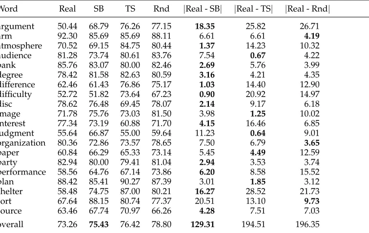
Recall performance of IMS on the 20 nouns of the Senseval-3 lexical-sample test set (Real column) compared with the corresponding similarity-based (SB), TS-based (TS), and random (Rnd) pseudowords. The last three columns show absolute differences between the real setting and the three pseudoword settings.

Word Real SB TS Rnd |Real - SB| |Real - TS| |Real - Rnd|

argument 50.44 68.79 76.26 77.15 18.35 25.82 26.71

arm 92.30 85.69 85.69 88.11 6.61 6.61 4.19

atmosphere 70.52 69.15 84.75 80.44 1.37 14.23 10.32

audience 81.28 73.74 80.61 83.76 7.54 0.67 4.22

bank 85.76 83.07 80.00 82.46 2.69 5.76 3.99

degree 78.42 81.58 82.63 80.59 3.16 4.21 4.35

difference 62.46 61.43 76.86 75.17 1.03 14.40 12.90

difficulty 52.72 51.82 73.64 67.23 0.90 20.92 14.97

disc 78.62 76.48 69.45 78.07 2.14 9.17 6.18

image 71.78 75.76 73.03 81.50 3.98 1.25 10.02

interest 77.34 73.19 60.88 71.70 4.15 16.46 6.85

judgment 55.64 66.87 55.00 59.64 11.23 0.64 9.01

organization 80.36 72.86 73.57 78.65 7.50 6.79 3.65

paper 60.84 66.29 65.33 73.14 5.45 4.49 12.59

party 82.94 80.00 79.41 81.04 2.94 3.53 3.74

performance 58.56 64.76 67.14 73.86 6.20 8.58 15.52

plan 88.42 85.41 90.27 87.39 3.01 1.85 3.12

shelter 58.48 74.75 87.00 80.21 16.27 28.52 21.73

sort 67.64 88.15 80.74 77.37 20.51 13.10 9.73

source 63.46 67.74 70.97 66.26 4.28 7.51 7.03

pseudowords (75.43) is closest to that of real words (73.26). This value is 76.42 and 78.80 for TS-based and random pseudowords, respectively.

In addition, for 12 of the 20 nouns, the similarity-based approach provides the pseudowords that are closest to real words in terms of WSD recall performance (|Real - SB| column in the table) as shown in bold in the table. This number drops to 5 and 3 for the TS-based and random pseudowords, respectively. Accordingly, the overall sum of the differences (distance) between the recall values is smallest (129.31) for similarity-based pseudowords among the three kinds of pseudoword (194.51 for TS-based pseudowords and an average of 196.35 for random pseudowords, ranging from 158.32 to 262.04).

Even though TS-based pseudowords are only 1% away from similarity-based pseu-dowords in terms of overall performance, their distance from real words is much higher than that of similarity-based pseudowords (194.51 vs. 129.31). This suggests that the former tend to have a lower correlation with real words than the latter. In the following, we investigate the correlation between the disambiguation difficulties of real words and our three types of pseudowords.

4.1.2 Correlation Between Disambiguation Difficulties.The smaller the angular deviation of the line of best fit for a set of pseudowords is from the diagonal line, the higher is the cor-relation between the disambiguation difficulties of those pseudowords and real words. As can be seen in the figure, the line corresponding to the similarity-based pseudowords has the smallest deviation from the diagonal line, showing its higher correlation with real words. The Pearson correlation coefficient between the disambiguation difficulties of similarity-based pseudowords and real words is 0.74. This value drops to 0.43 and 0.54 for TS-based and random pseudowords, respectively. Even worse, the value of 0.54 is the average of 25 highly variable correlation values (in the range of [0.18, 0.67]) over our 25 sets of random pseudowords. The reason why TS-based pseudowords show a lower correlation than random pseudowords can be found in the fact that the reported values for the latter are averaged over 25 runs. More precisely, the correlation value of 0.43 of topic signatures has to be compared with the range [0.18, 0.67] of correlations obtained by different sets of random pseudowords.

4.1.3 Discussion.We leveraged PPR and topic signatures as our sense modeling compo-nents for the generation of semantically aware pseudowords. Both approaches could solve the low coverage problem, although the results presented in this section suggest that the topic signature-based approach is not good at providing suitable monosemous substitutes for senses of real ambiguous words. A closer look at the similarity-based and TS-based pseudowords generated for some of the nouns in the Senseval-3 data set, shown in Table 8, provides a clear explanation for this shortcoming of topic signature-based pseudowords. In fact, topic signatures are signature-based on co-occurrence information from the Web snippets retrieved for each sense of an ambiguous noun. As a result, many of the top-ranking words in each topic signature are syntagmatically related to the given sense. For example, consider the paralysispseudosense of arm, europeanpseudosense ofplan, andmoralorweeklypseudosenses ofpaper. Despite being semantically related, these pseudosenses cannot be considered as good substitutes for their correspond-ing senses. Our similarity-based approach, instead, tends to favor paradigmatic (i.e., taxonomic) relations, which is, in fact, the reason behind its better ability at finding suitable substitutes for senses of real words.

Table 8

The similarity-based (SB) and TS-based (TS) pseudowords obtained for 6 of the 20 nouns used in our disambiguation experiment.

word type: equivalent pseudoword

difficulty SB: workout*deterrent*predicament*complexity

TS: get*autism*ski*credibility

arm SB: forearm*baseball cap*sword*armchair*executive branch*garment

TS: paralysis*glue*weaponry*wheelchair*pension*clothing

plan SB: retirement plan*architect*diagram

TS: employee*european*pale

performance SB: concert*encore*achievement*feat*processing TS: theatrical*musical*ballroom*recruitment*steady

party SB: political party*dinner party*clique*fiesta*someone

TS: socialist*prom*transaction*coronation*boomer

paper SB: piece of paper*papers*news story*telecom*editorial*publishing house*movie

TS: towel*moral*vitamin*brochure*weekly*firm*forecast

of large-scale data sets for our experiments. Hence, we do not consider this type of pseudoword in our further evaluations and focus on similarity-based pseudowords only.

4.2 Representative Power of Pseudosenses

In order to maximize the possibility of preserving the meaning of the original synset, a pseudosense should be selected from the set of words in the same synset, or in the directly related synsets (e.g., hypernym synsets). However, many of the WordNet synsets do not contain monosemous terms and the similarity-based approach often needs to look further into the other indirectly related synsets so as to find a suitable pseudosense. In order to assess how often this happens, we carried out an experiment to get a clear idea of the exact statistics on the distances of the synsets from which pseudosenses are selected from the synsets containing the original senses. To this end, we went through all our similarity-based pseudowords and, for each pseudosense

wi, checked the relationship in WordNet between the synset containing wi and the corresponding real sense.

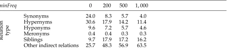
We show in Table 9 how the pseudosenses are distributed across different types of WordNet relations, including indirect ones. As can be seen in the table, whenminFreq

Table 9

Percentage of similarity-based pseudosenses obtained from different types of WordNet relations.

minFreq 0 200 500 1, 000

Relation type

Synonyms 24.0 8.3 5.7 4.0

Hypernyms 30.6 17.9 14.2 11.4

Hyponyms 9.6 7.2 5.7 4.6

Meronyms 0.4 0.4 0.3 0.3

Siblings 9.7 17.9 17.2 16.2

Table 10

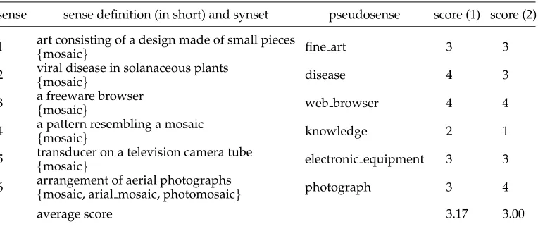
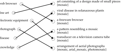
Examples for representativeness scores assigned by the two annotators to pseudosenses of the termmosaic.

sense sense definition (in short) and synset pseudosense score (1) score (2)

1 art consisting of a design made of small pieces_{ fine art 3 3

mosaic}

2 viral disease in solanaceous plants_{ disease 4 3

mosaic}

3 a freeware browser_{ web browser 4 4

mosaic}

4 a pattern resembling a mosaic_{ knowledge 2 1

mosaic}

5 transducer on a television camera tube_{ electronic equipment 3 3

mosaic}

6 arrangement of aerial photographs_{{mosaic, arial mosaic, photomosaic}} photograph 3 4

average score 3.17 3.00

is set to 1, 000, only about 20% of the pseudosenses are picked out from synonyms or generalization/specialization relations (hypernym and hyponyms). This shows that a considerable portion of our pseudosenses are selected from synsets that are indirectly related to the target synset that is being modeled. These indirectly related synsets can potentially result in pseudosenses that do not have very similar meanings to the original synsets, and hence are not good representatives of them.

Having observed this, we carried out an experiment to evaluate the representative power of similarity-based pseudosenses to assess how well each pseudosense models its corresponding real sense. For this purpose, we randomly sampled 10 pseudowords for each degree of polysemy from 2 to 12 from the entire set of pseudowords6generated with minimum frequency of 1,000, totaling 110 pseudowords with 770 pseudosenses. We then asked two annotators, neither of whom was an author of this paper, to judge the representative power of each pseudosense according to the following scale: 1 (com-pletely unrelated), 2 (somewhat related), 3 (good substitute), 4 (perfect substitute). The annotators were provided with the WordNet definitions of the corresponding synsets.

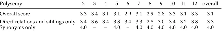
As an example, consider the pseudowords corresponding to the nounmosaicshown in Table 10. We present in the table the representativeness scores given by each of our annotators to the individual pseudosenses of this word. The overall representativeness score is calculated as the average of the scores given by the two annotators. In the case of our example, the overall score is 3.085. We also calculated the Spearman correlation between the scores given by the two annotators for all the 770 cases to be 0.66. We show in Table 11 (top) the overall representativeness scores averaged for the full set of 770 pseudosenses, classified by polysemy degree. As can be seen from the table, the overall representative score remains around 3.0 for all polysemy degrees from 2 to 12, with the overall score being 3.1. This shows that even though about 64% of the pseudosenses are picked out from indirect relations (when minimum frequency is 1,000, cf. Table 9), they can still be considered as good representatives for their corresponding real senses. We also present in Table 11 (bottom) the average representativeness scores only for

Table 11

Average representativeness scores for pseudosenses of different polysemy classes (scores range from 1 to 4) and from different WordNet relations. We also show, in the last two rows, the average scores for only those pseudosenses that are picked from synonyms or directly related and sibling synsets.

Polysemy 2 3 4 5 6 7 8 9 10 11 12 overall

Overall score 3.3 3.4 3.1 3.1 2.9 3.1 2.9 2.8 3.3 3.1 3.3 3.1

Direct relations and siblings only 3.4 3.6 3.4 3.3 3.4 3.3 2.8 3.0 3.4 3.2 3.8 3.3

Synonyms only 4.0 – – 4.0 – 4.0 4.0 4.0 4.0 4.0 4.0 4.0

those pseudosenses that are picked from words in the same synset (synonyms) or in the directly related and sibling synsets. As can be seen, the synonymous pseudosenses are always rated with the highest possible score of 4, whereas those obtained from direct relations maintain a relatively higher score compared with the overall repre-sentative score, which includes many pseudosenses picked from indirect relations. In fact, the similarity-based pseudoword generation approach improves the vicinity-based method to full coverage and provides a significantly better level of flexibility for higher values of minimum frequency, while maintaining a good degree of sense modeling ability.

4.3 Distinguishability Between Pseudosenses

A fundamental property of an ambiguous word is that its different senses have distinct meanings. We expect a semantically aware pseudoword to inherit this property of its real counterpart (i.e., to have pseudosenses that are semantically distinguishable from each other while being semantically similar to their corresponding senses). As an exam-ple, consider the similarity-based pseudowordphilanthropist*benefactor7corresponding to the noun donor.8 The two pseudosenses of the pseudoword can be considered as good representatives for their corresponding senses. However, the distinguishability of the two real senses is not preserved in the corresponding pseudoword: whereas

philanthropist only applies to the first sense, benefactor can be equally good for both senses ofdonor.

Hence, we performed another evaluation in order to determine the degree of the distinguishability of pseudosenses of our pseudowords. For this evaluation, we used the same set of 110 pseudowords as in the previous experiment (Section 4.2). For each of these pseudowords, we presented its pseudosenses in random order to two annotators. In addition, we provided these annotators with the WordNet definitions of the senses of the corresponding noun and asked them to associate each pseudosense with the most appropriate WordNet sense. The annotators were instructed to leave a pseudosense unmapped if they found it to be equally mappable to multiple senses. We then calculated the distinguishability score for each polysemy degree as the ratio of the number of correct mappings to the total number of senses.

7 From WordNet: “Philanthropist: someone who makes charitable donations intended to increase human well-being”; “Benefactor: a person who helps people or institutions (especially with financial help).” 8 The termdonorhas two senses according to WordNet 3.0: (1) “person who makes a gift of property”;

web browser

fine art

electronic equipment

photograph

disease

knowledge

art consisting of a design made of small pieces {mosaic}

viral disease in solanaceous plants {mosaic}

a freeware browser {mosaic}

a pattern resembling a mosaic {mosaic}

transducer on a television camera tube {mosaic}

arrangement of aerial photographs {mosaic, arial_mosaic, photomosaic}

Figure 2

Mappings provided by an annotator from pseudosenses of the similarity-based pseudoword

for the nounmosaicto its real senses (as defined in WordNet 3.0). In this case all mappings are

correct and hence the distinguishability score for this pseudoword will be 6/6=1.

For instance, consider the noun mosaicthat has six senses in WordNet 3.0. As we also saw in the previous experiment, the corresponding similarity-based pseudoword for this noun isfine art*disease*web browser*knowledge*electronic equipment*photograph. As illustrated in Figure 2, we provided the shuffled list of pseudosenses of this pseu-doword (left column) and the WordNet definitions of the senses of its corresponding noun, namely,mosaic(right column), to each annotator and asked them to map each pseudosense to its most suitable real sense. In this case, both annotators mapped all pseudosenses to their correct senses; hence, the distinguishability score given by each annotator for this pseudoword was 6/6 = 1.

We show in Table 12 the average distinguishability scores for each degree of poly-semy 2 to 12 as well as the overall score that is calculated as the average of per-polysemy scores. As can be seen in the table, the distinguishability score is inversely proportional to the polysemy degree (there is a high negative Pearson correlation of 0.9 between the two). However, the score remains above 0.70 even for the pseudowords with higher polysemous degrees. The overall score of 0.79 shows that a large portion of pseudosenses can be associated with their corresponding real senses only. Therefore we can conclude that the similarity-based pseudowords effectively preserve the distin-guishability of senses of their real counterparts.

4.4 Discussion

We performed three experiments to evaluate the reliability of our pseudowords. We showed that the similarity-based pseudowords are fairly close to their real counterparts in terms of disambiguation difficulty. Even though our similarity-based pseudowords were slightly easier to disambiguate in comparison to real words, the high correlation observed in the first evaluation (Section 4.1) serves as a guarantee that our pseudowords

Table 12

Average distinguishability scores for pseudosenses of different polysemy classes (scores range from 0 to 1).

Polysemy 2 3 4 5 6 7 8 9 10 11 12 overall

can be reliable substitutes for real words in experiments concerning the analysis and comparison of WSD systems.

Our further experiments provided manual evaluations of the representativeness of individual pseudosenses of our similarity-based pseudowords as well as the distin-guishability of their pseudosenses from one another. In the representativeness exper-iment, we assessed, for each individual sense of each pseudoword in our sample set, if the meaning of the corresponding real sense is preserved and if each pseudosense can be considered as a good representative of its corresponding real sense. Finally, in the distinguishability experiment our aim was to investigate the ability of similarity-based pseudowords at preserving the distinguishability among senses of real words. Experimental results proved that the similarity-based approach is able to provide a good modeling of individual senses of real words while preserving the distinguishability of their senses.

5. Sampling Pseudosense-Tagged Corpora

As a result of our evaluations we know that the similarity-based pseudowords are reliable substitutes for real ambiguous words in the disambiguation task. As described in Section 3, a pseudosense-tagged corpus can be generated for each pseudoword

p=w1∗w2∗. . .∗wn by substituting individual occurrences of its pseudosenses wi with the pseudowordpitself, while marking the pseudosensewias its annotation. An obvious question that arises here is how to sample and distribute the sentences for a pseudoword across its pseudosenses. In the following two sections we illustrate two corpus sampling strategies used in our experiments.

5.1 Uniform Sense Distribution

A first, simple sampling strategy for pseudosense-tagged corpora is the uniform sense distribution. In this setting, all senses of a pseudoword are assumed to be observed with equal probability in the tagged corpus (i.e., we extract the same number of sentences from the corpus for each pseudosense of a given pseudoword).

5.2 Natural Sense Distribution

Table 13

Number of distinct nouns annotated in SemCor at least 1, 10, or 20 times. We also show the total number of WordNet ambiguous nouns (last row) for different polysemy degrees.

Polysemy 2 3 4 5 6 7 8 9 10 11 12 >12 total

Frequency≥1 2,349 1,315 703 453 241 183 81 91 57 45 23 49 5,590

Frequency≥10 301 242 196 180 122 97 61 60 43 35 20 43 1,400

Frequency≥20 122 97 112 111 70 63 47 42 29 24 15 35 767

WN amb. nouns 10,257 2,989 1,178 620 306 212 96 94 60 48 25 50 15,935

Table 14

Average sense distribution for nouns in SemCor. We select only those nouns for which there exist at least 10 sense-tagged occurrences in SemCor.

Poly. p1 p2 p3 p4 p5 p6 p7 p8 p9 p10 p11 p12

2 87.8 12.2

3 78.1 17.9 4.0

4 72.9 19.6 6.4 1.1

5 71.1 18.8 7.4 2.3 0.4

6 65.4 21.5 8.5 3.1 1.2 0.3

7 61.1 23.0 9.5 4.1 1.8 0.4 0.1

8 62.7 20.9 9.3 4.4 1.8 0.6 0.2 0.1

9 56.0 22.4 10.4 5.6 3.4 1.6 0.6 0.0 0.0

10 51.1 24.4 11.7 7.0 3.6 1.4 0.6 0.2 0.0 0.0

11 50.7 23.5 12.0 6.8 3.6 1.7 1.0 0.4 0.2 0.1 0.0

12 54.3 18.2 9.1 7.2 4.4 2.7 2.1 1.4 0.5 0.1 0.0 0.0

low-polysemy nouns and a few dozen high-polysemy nouns, we decided to drop the requirement of estimating sense distributions directly (i.e., to model the semantically aware pseudowordpwon the sense distribution ofw). Instead, we first collected all the sense distributions of nouns with at least 10 occurrences in SemCor. Our choice of 10 as the minimum occurrence frequency was to guarantee some hundreds of distributions for lower polysemy degrees and dozens for the higher ones (see Table 13). In addition, given the highly skewed nature of sense distributions in SemCor, 10 samples should usually be enough for a reliable estimation of the corresponding sense distributions to be made, even for higher polysemy degrees. Having at hand a large set of distri-butions estimated for each polysemy degree, every time we needed a new pseudo-word withmsenses, we randomly picked out a sense distribution of sizemfrom our collection.

We show the macro-averaged9 _{sense distribution for each polysemy degree from}

2 to 12 in Table 14. As can be seen from the table, all average distributions, especially those of low polysemy nouns, are skewed towards predominant senses.

6. Experimental Set-up

In this article up to this point we have provided the basis for creating large-scale pseudosenannotated data sets by proposing a flexible approach for generating se-mantically aware pseudowords that model arbitrary real words. We have also ex-plained different sampling strategies for distributing pseudosense-annotated sentences according to two different distributions. We are now ready to set up our experimental framework for large-scale WSD.

We first describe the text corpus used in our experiments (Section 6.1), then explain how we selected a reliable subset of pseudowords for the experiments (Section 6.2); this is followed by a description of the process of generating training and test data sets (Section 6.3). In Section 6.4 we introduce the two WSD systems used as representatives of the two main WSD paradigms (i.e., supervised and knowledge-based) in our experi-ments. We then provide, in Section 6.5, the details of the method through application of which our knowledge-based system is able to benefit from the training data. Finally, in Section 6.6 we describe the evaluation measures used in our experiments.

6.1 Corpus

We sampled all the sentences for pseudosense tagging from the English Gigaword pus (Graff and Cieri 2003), a comprehensive corpus of English newswire text. The cor-pus comprises about 4.1 million documents, each containing an average of 430 words, totaling approximately 1.76 billion words. In a preprocessing phase, we removed sen-tences whose length was either longer than 50 words or shorter than 10 words. The corpus was then annotated with part-of-speech tags using the C&C tagger (Curran and Clark 2003) trained on the Penn Treebank (Marcus et al. 1994). The resulting corpus contained around 50 million sentences.

6.2 Pseudoword Selection

As a result of our similarity-based approach, we could generate as many pseudowords as polysemous nouns in WordNet 3.0 (i.e., 15,935 pseudowords). However, for two reasons that will be explained shortly, we only considered a reliable subset of these pseudowords for generating the data sets for our experiments.

Firstly, we did not consider nouns with polysemy degree higher than 12 in our experiments, as it is not possible to perform a reliable analysis on such degrees given that very few pseudowords can be generated for them (about 0.3% of ambiguous nouns in WordNet have polysemy degree 13 or higher). Secondly, we observed that in practice a large enough portion of pseudowords for each polysemy degree can provide a reliable performance estimation on that polysemy degree. Therefore, we selected, for each polysemy degree, the top 300 pseudowords according to the calculatedaverageRank