Multinomial Least Angle Regression with Application to Web Personalization

Multinomial Least Angle Regression with

Application to Web Personalization

Ilya Gluhovsky

Abstract—Keerthi and Shevade (2007) proposed an efficient algorithm for constructing an approximate LARS solution path for logistic regression as a function of the regulariza-tion parameter. In this paper we extend their approach to multinomial regression. We show that a brute-force approach leads to a multivariate approximation problem resulting in an infeasible path tracking algorithm. Instead, we introduce a non-canonical link function thereby a) repeatedly reusing the univariate approximation of Keerthi and Shevade and b) producing an optimization objective with a block-diagonal Hessian. We carry out a simulation study that shows the computational efficiency of the proposed technique. A Matlab implementation is available from the author upon request. We apply this technique to a web personalization problem in corporate marketing.

Index Terms—Machine learning, supervised learning, gen-eralized linear models (GLM), least angle regression and LASSO (LARS), least absolute shrinkage and selection operator (LASSO), large-scale regression, solution path tracking.

I. INTRODUCTION

W

K-class classification problem. Let {(xi, y_i), 1 ≤ i≤N} denote the training data set. It is assumed to be an independent, identically distributed sample of(X, Y), a data pair of a predictor vector X and a response Y that takes values in the set{1,2,· · ·, K}of class labels. Furthermore, the conditional distribution ofY is assumed to be

Y|X=x∼Multinomial(p₁(x),· · ·, p_K(x)),

wherep_k(x)are unknown conditional class probabilities

p_k(x) =P{Y =k|X=x}

for a predictor realization x. Our goal is to estimate the

p_k(x).

We adopt a generalized linear model [1] with link function

ρ, so that

p_k(x, β) =P{Y =k|x, β) =ρ_k

xT_β(1)_{,· · ·,x}T_β(K)_. The purpose of the link function in a generalized linear model is to map the linear predictors, in this case xTβ(k),1 ≤ k ≤ K, into the mean of the response distribution, in this case p_k(x, β),1 ≤ k ≤ K. In particular, the p_k are now parameterized by β =β(1),· · ·, β(K), the unknown parameter vector that determines the model, where β(k)

denotes the parameter vector corresponding to class k with

β(K)≡0by convention to remove ambiguity introduced by the constraint_kp_k(x, β) = 1. A typical choice ofρis the canonical link [1]

p_k(x, β) = exp

xT_β(k)

_K

l=1exp

xT_β(l). (1) I. Gluhovsky is Chief Scientist, Ancestry.com Inc., San Francisco, CA 94107, [email protected], [email protected]

Manuscript received February 02, 2011; revised April 19, 2011.

As a criterion of findingβ, we pose the penalized likeli-hood problem

min

β fλ(β), (2)

where

f_λ(β) =f₀(β) +λ||β||₁ (3)

and

f₀(β) = μ

2βTAβ−

N

i=1

logp_yi(xi, β) (4)

is the sum of an L₂ regularization penalty and a negative log-likelihood. The regularization penalty matrix A is any positive semidefinite matrix, such as the identity or a kernel penalty matrix [2]. Thus, our regularization introduces both an L₁ penalty in (3) and an L₂ penalty in (4), a so-called elastic net proposed in [3]. While μ is fixed at a small value as in [3], our task is to compute the solution

ˆ

β(λ) as a function of the L₁ penalty weight λ known as a regularization parameter as the latter varies over the nonnegative numbers. We will refer to βˆ(λ)as the solution path.

When λ is very large, βˆ(λ) = 0 as the L₁ penalty dominates. As λ decreases, more and more coordinates of

β become nonzero, typically one at a time leading to sparse solutions forinterestingvalues of λ. This is contrasted with using a single L₂ penalty where typically all coefficients

ˆ

β(λ) become nonzero simultaneously [4], [5]. The latter choice results in many small coefficients which are typi-cally estimated with high variance. Therefore, L₁ penalty solutions are often superior in estimation accuracy [5]. A sparse solution also offers important practical advantages as a production system that uses one needs to concern itself with generating only a subset of predictors in real time, so that online model evaluations become faster. Finally, as

λ approaches zero, βˆ(λ) approaches the minimizer of (4), which is the maximum likelihood solution subject to the small L₂ penalty.

Spearheaded by seminal research [4], efficient algorithms for constructing the entire solution path for all values of λ

were proposed in [2], [5], [6]. Advantages of solution path tracking include a) sorting the predictors by their importance based on the order in which they enter the model as λ de-creases and b) choosing the best fit in the entire solution path (e.g. by cross-validation) having yielded all the parameter vectors, which are calculated in one pass by the procedure. The computational complexity of path-tracking algorithms is comparable to that of a single-λ optimization [5]. This result is concurred in practice by [7] showing that running times of path tracking are not much worse than those of single-λcompetitors. Since selecting theλtypically involves running the latter with many trial values, path tracking offers a significantly better quality/running-time tradeoff than a

one-λ-at-a-time optimization heuristic. Our empirical study in Section V verifies this property for the proposed path tracking algorithm.

Inclusion of theL₁penalty into a fitting criterion was first treated in detail in [8], where it was dubbedLASSO. [4], [5] proposed a path-tracking method called least angle regres-sion and LASSO(LARS) for squared-error loglikelihood (as in linear regression solved by ordinary least squares) whose simple modification in particular yields the entire LASSO solution path. [6] extended the technique to generalized regression models with piecewise-quadratic loglikelihood. [2] proposed an efficient approximation method that reduces the logistic regression problem to the setting in [6].

Path tracking is based on the following observation. When-ever the functionf₀ in (4) is piecewise quadratic in β, the solution path βˆ(λ) is piecewise linear. At each step, [6] calculates the direction of a new segment and the extent to which the solution path follows the segment. [2] specializes to logistic regression, which is a special case of multinomial regression with the number of classesK= 2. In order to use the path tracking algorithm in [6], [2] proposes a particular piecewise quadratic approximation to the loglikelihood in (4). Additionally, [2] proposes a pseudo-Newton correction process applied after the original path construction to reduce the impact of the approximation and move closer to the true path.

In this paper we propose an approximate path tracking method for multinomial regression. To the best of our knowledge, this is the first multinomial least angle regression method. We now outline the specifics of our contribution. To find a piecewise quadratic approximation tof₀(β)in (4), it is sufficient to approximate the summandslogp_yi(xi, β). Using the canonical link (1), the latter is equivalent to approximating

logexpxT_β(1)_{+· · ·+ expx}T_β(K−1)_{+ 1 (5)} since the logarithm of the numerator of (1) is already linear inβ andβ(K)≡0. In the logistic case of K= 2, [2] finds a tight piecewise quadratic approximantˆl(r)to a univariate function

l(r) = log1 +e−r (6) depicted in Figure I. Since r = −xTβ(1) is linear in β, this not only offers the sought-after approximation, but also leads to an efficient step for determining the approximation segment for any particularr_i = xT_iβ(1). This efficiency is critical for computational feasibility because the direction of the solution path is recomputed every time any of ther_ihits a segment endpoint along with the magnitude of the extension of the path in the new direction. Therefore, the extension computation is frequent and has to be performed for every data point every time. For medium-size datasets in Section V, a typical number of such computations is 100 million for constructing the entire solution path.

Let us now examine an analogous approach in the case of

K >2. Withr_k =xTβ(k)in (5) we would have to introduce an approximation to a(K−1)-variate function

l_K(r₁,· · ·, r_K−1) = log(1 +e−r1+· · ·+_e−rK−1)_{. (7)}

Dealing with complex(K−1)-dimensional approximation regions in place of one-dimensional segments would lead to

Fig. 1. l(r)(black solid) and its piecewise quadratic approximant ˆl(r) (dashed red). Reproduced from [2].

TABLE I

APPROXIMATION SEGMENTS USED TO DEFINEˆl(r)IN(8)ALONG WITH THE CORRESPONDING VALUES OF THE PIECEWISE CONSTANT

COEFFICIENTa(r).

r (−∞,−4] (−4,−1.65] (−1.65,1.65] (1.65,4] (4,∞)

a(r) 0 0.0618 .215 0.0618 0

an infeasible algorithm for data sets of moderate sizes as discussed in Section IV.

We solve this problem by proposing a particular non-canonical link function in place of (1). This allows us to continue using a univariate approximation to (6) applied up toK−1 times for each data point. This link function also produces an optimization objective with a block-diagonal Hessian with K −1 blocks. These two benefits lead to algorithmic efficiency similar to that of [2] in the multinomial setting.

In Section II we give details of the proposed link function and the ensuing piecewise-quadratic approximation to the loglikelihood. The path tracking algorithm is described in Section III. In Section IV we further contrast our algorithm with a brute-force approach leading to the (K−1)-variate approximation outlined above. In Section V we carry out a brief simulation study that illustrates the computational effi-ciency of the proposed algorithm as discussed above across various numbers N, P, and K of observations, predictor variables, and class labels respectively. In Section VI we apply the techinique to a web personalization problem in corporate marketing. We conclude in Section VII.

II. NEWLINKFUNCTION AND APIECEWISEQUADRATIC APPROXIMATION TOLOGLIKELIHOOD

[2] proposes a particular nonnegative, convex, contin-uously differentiable, and piecewise quadratic approximant

ˆ

l(r) to l(r) in (6). These properties meet the requirements of the path tracking algorithm in [6]. Figure I illustrates its tightness achieved with just 5 approximation segments that make up the horizontal axis and are given in the first row in

Table I.ˆl(r)is given by

ˆ

l(r) = (1/2)a(r)r2+b(r)r+c(r) (8)

witha(r), b(r),andc(r)being constant within each segment. In particular,ˆl(r)is linear over(−∞,−4]with the slope of

−1 and is zero over[4,+∞). Only the values ofa(r)given in Table I are used in the path tracking algorithm in Section 3. Other details are available in [2].

We now introduce the new link function that allows us to approximate the multinomial loglikelihood by only involving this univariate ˆl(r) and not its multivariate counterparts as outlined above and detailed in Section IV. It is defined by

_k

l=1pl(x, β)

k+1

l=1 pl(x, β)

= 1

1 + exp−xT_β(k), k= 1,· · ·, K−1 (9) or equivalently,

p_k+1(x, β)

_k+1

l=1 pl(x, β)

= 1

1 + expxT_β(k), k= 1,· · ·, K−1. Thus, the linear predictor η_k = xTβ(k) determines the fraction ofP{Y =k+1|x, β}inP{Y ≤k+1|x, β}. This is known asstick-breaking constructionoften used in conjunc-tion with Dirichlet processes1. In particular, any distribution

{p₁(x, β),· · ·, p_K(x, β)} can be represented by (9) for the appropriate choice of linear predictors {η₁,· · ·, η_K} and, conversely, any choice of the linear predictors corresponds to a valid distribution {p₁(x, β),· · ·, p_K(x, β)} obtained through (9).

Below we use the convention that an empty product is one and an empty sum is zero. Thep_k can be recovered by

p₁(x, β) =

K−1 m=1

1

1 + exp−xT_β(m), and fork≥2,

p_k(x, β) =

k

l=1

p_l(x, β)−

k−1

l=1

p_l(x, β) =

K−1 m=k

1

1 + exp−xT_β(m)− K−1 m=k−1

1

1 + exp−xT_β(m) =

=

K−1 m=k

1

1 + exp−xT_β(m)

1−_{1 + exp} 1

−xT_β(k−1)

= = K−1 m=k 1

1 + exp−xT_β(m)

1

1 + expxT_β(k−1)

.

These factorizations enable us to express the loglikelihood summands in (4) in terms ofl in (6) by

logp₁(x, β) =−

K−1 m=1

l

xT_β(m)_,

logp_k(x, β) =−

K−1 m=k

l

xT_β(m)_−l−xT_β(k−1)_{, k≥2} (10)

1_{http://en.wikipedia.org/wiki/Dirichlet process#The}

stick-breaking process

Thus, a piecewise quadratic approximation to the univariate

l(r)induces that to the penalized loglikelihood in (4). This allows for a computationally efficient path tracking algorithm that we describe next.

III. PATHTRACKINGALGORITHM The hat quantities in the new minimization objective

min

β

ˆ

f_λ(β), (11)

with

ˆ

f_λ(β) = ˆf₀(β) +λ||β||₁ (12)

are obtained from (2)-(4) by using the approximationˆl(r)in place of l(r)in (10) and substituting these into (4):

ˆ

f₀(β) = μ

2βTAβ+

N

i=1

K−1 k=max(1,yi−1)

ˆ

l(r_ik), (13)

wherer_ik =s_ikx_iβ(k)withs_ik = 1ify_i≤kands_ik =−1

if y_i =k+ 1. The gradientgˆ and the Hessian Hˆ offˆ₀ are given by ˆ g β(k)

=μA_kβ(k)+

N

i=1

1{yi≤k+1}sikxi[a(rik)rik+b(rik)]

(14) and

ˆ H

β(k), β(k)

=μA_k+

N

i=1

1{yi≤k+1}xixTia(rik)

ˆ H

β(k), β(l)

=0, k=l, (15)

wheregˆβ(k)refers to the vector of partial derivatives with respect to β(k),Hˆ β(k), β(l) is the block ofHˆ with rows (columns) corresponding toβ(k) (β(l)), and we assume that theL₂penalty matrixAis block-diagonal with the rows and columns of block A_k corresponding to β(k). We also used the fact that ˆl is piecewise quadratic with coefficients a, b, andc (the latter is not used) as given by (8).

Given the gradient and the Hessian, we can apply the path tracking algorithm of [2], [6]. We now outline its justification and main steps. The Karush-Kuhn-Tucker conditions [6] imply that for any parameter β_j, either it is inactive with

β_j= 0and|gˆ_j| ≤λor it is active (β_j = 0) with

ˆ

g_j=−λsgn(β_j), (16)

where sgn(β_j)is the sign ofβ_j. Let Abe the set of active parameters and use notationxAandB_Ato denote the vector

x_j, j∈ Aand the block of matrixB with rows and columns fromA respectively.

Sincefˆ₀ is piecewise quadratic (or from (14) and (15)), a change in β andgˆ are related byδˆg= ˆHδβ. Settingδλ= −1, (16) implies that

δβ_A= ˆH_A−1δˆg_A= ˆH_A−1sgn(β_A) =−Hˆ_A−1sgn(ˆg_A).

Thus, as λ decreases, the solution path extends in the direction above implying in particular its piecewise linearity. The linear extension continues until either a) a new parameter j becomes active with |gˆ_j| = λ; b) a parameter reaches zero; or c) the path reaches a piecewise quadratic approximation segment endpoint for any of the

r_ik in (13). When either of these events happens, the direction of the path is recalculated. The complete algorithm whose description closely parallels that in [2] is given below.

Path Tracking Algorithm

Initialize: β = 0, r_ik = 0, a_i = a(0) ∀i,

ˆ

gβ(k)= 0 = −(1/2)N_i=11_{yi≤k+1}s_ikxi, A = argmax_j|gˆ_j|, λ = max_j|ˆg_j|, δβ_A = −Hˆ_A−1sgn(ˆg_A),

δβ_Ac = 0, δr_ik = s_ikx_iδβ(k) for i : y_i ≤ k+ 1, and δˆg= ˆHδβ.

While (λ >0)

a)d₁= min{d >0 : |gˆ_j+dδˆg_j|=λ−d, j∈ Ac}; b)d₂= min{d >0 :β_j+dδβ_j = 0, j∈ A};

c)d₃= min{d >0 :r_ik+dδr_ikreaches an approximation segment endpoint for somei, k};

d)d = min{d₁, d₂, d₃}, λ ← λ−d, β ← β +δβ, r ← r+δr,gˆ←dδgˆ;

e) ifd=d₁, add the parameter attaining equality atd to

A;

f) ifd=d₂, remove the coefficient attaining 0 at dfrom

A;

g) ifd =d₃ at (i∗, k∗), set a(r_i∗_k∗) to the value in the new segment;

h) set δβ_A = −Hˆ_A−1sgn(ˆg_A), δβ_Ac = 0, δr_ik =s_ikxiδβ(k) fori: y_i≤k+ 1,andδgˆ= ˆHδβ.

At each iteration, most of the time is spent updating the inverse of the Hessian in h). This is typically done by maintaining and updating the Cholesky decomposition of the Hessian. Because of the block-diagonal form of the Hessian in (15), one only needs to manipulate and invert the individual blocks Hˆβ(k), β(k). Also, a single parameter addition and removal in steps e) and f) as well as a single change for a (i∗, k∗) pair in g) entails an update of only a single block of the Hessian since only a single k∗ is affected. By contrast, if the canonical link (1) were to be used, it could be seen that differentiating (5) with respect to

∂β(k)∂β(l), k =l would not produce zero. Therefore, one does not obtain a block-diagonal Hessian in the canonical link case.

Finding thedin c) for each(i∗, k∗)pair is a simple closed-form computation. This is thanks to using the univariate approximation whose approximation regions are segments. In the next section we contrast this simplicity with the complexity of using(K−1)-variate approximation regions which would ensue if the canonical link (1) were to be employed.

IV. MULTIVARIATEAPPROXIMATION WITHCANONICAL LINK

To further emphasize the importance of choosing the pro-posed link function, we pause here to review the difficulties which would be caused by using the canonical link (1). As discussed above, a parallel approach would be to approximate

l_K in (7) with a piecewise quadratic function. In the case of

K = 3, Figure II depicts l₃(r₁, r₂). l₃ can be seen to be highly non-additive. That is, there are no functions a₁(r₁)

and a₂(r₂) whose sum adequately approximatesl₃(r₁, r₂). For if it were the case, the graphs ofl₃(−5, r₂)andl₃(5, r₂)

Fig. 2. l₃(r₁, r₂), a special case of (7) forK= 3

Fig. 3. Mixed partial derivative∂l₃(r₁, r₂)/∂r₁∂r₂

againstr₂marked by arrows in Figure II would have approx-imately the same shape, namely that of a₂(r₂), and would only differ in their vertical positions. Therefore, an additive expansion similar to (10) enjoyed in the proposed link case which would allow for univariate approximations to a₁(r₁)

anda₂(r₂)is not possible.

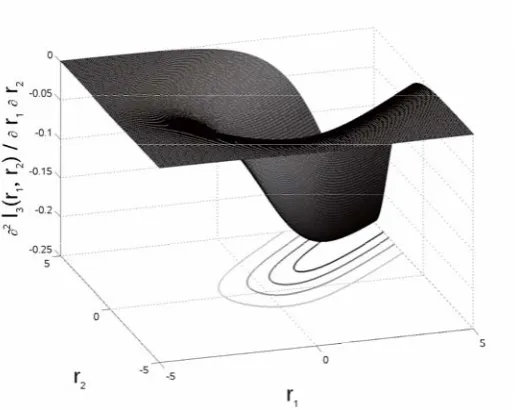
Alternatively, one may attempt to develop a (K −1) -dimensional piecewise quadratic approximation, where the “pieces” are proper (K−1)-dimensional regions. A com-putational infeasibility of this approach for large training datasets lies in the step c) of the algorithm above, where the distance dto reach the boundary of the current “piece” has to be computed for every training data point. Since tracking multivariate boundaries is tricky regardless of their shapes, this is not a scalable proposition. Nevertheless, let us examine the mixed second derivative∂l₃(r₁, r₂)/∂r₁∂r₂

depicted in Figure III. A piecewise quadratic approximation has a piecewise constant second derivative. Therefore, the

TABLE II

AVERAGE RUNNING TIMES FORmnrfit(MAXIMUM LIKELIHOOD ONLY,

NO REGULARIZATION), TMPM (L1REGULARIZATION FOR A SINGLEλ),

AND MULTINOMIALLARSAS DESCRIBED IN THIS WORK ACROSS SIMULATED DATASETS VARYING IN THE NUMBER OF OBSERVATIONSN,

PREDICTOR VARIABLESP,AND CLASS LABELSK.

Datasets Running Times

N P K mnrfit TMPM LARS

100K 50 3 1,004.2 690.9 1,971.7 50K 20 6 174.9 640.4 1,600.8 10K 10 24 133.6 3433.3 1306.2 10K 20 12 104.6 369.9 630.1 10K 100 3 82.4 25.2 80.2

4K 10 12 15.5 216.1 35.6 10K 20 3 6.85 17.89 3.18

2K 10 6 1.87 5.61 1.43

1K 10 3 .421 .562 .090

boundaries of an accurate approximation should generally follow the contour curves in Figure III. A convoluted shape of these contour curves only adds to the boundary tracking problem. These difficulties are expected to become even more pronounced asK grows.

V. EMPIRICALEVALUATION

In this section we report the results of a brief computa-tional performance comparison study of our Matlab imple-mentation of the path-tracking algorithm with the proposed link function against two competitors: the standard Matlab multinomial regression routinemnrfitand a publicly available Matlab implementation2 _{of a two-metric projection method}

(TMPM) with non-negative variables [7], [9]. Note that mnr-fitaims at finding the maximum likelihood solution, but does not carry out anyL₁ regularization. TMPM does carry out

L₁ regularization, but only attempts to solve the regularized problem (2) for aparticularλas opposed to finding the full solution path as in our technique. Therefore, our primary question in this study is how much more computationally expensive it is to obtain the full regularized solution path.

We generate simulation datasets for various numbersN,

P, and K of observations, predictor variables, and class labels respectively. In order to run these simulations on a commodity laptop with 2GB of RAM, we generate sparse matrices X of size N × P with the 2.5% fraction of nonzero entries sampled uniformly from[0,1]. Furthermore, upon generating the true coefficient vector β also sampled uniformly from[0,1], for each rowx_iof X we apply the link function to the linear predictorsxT_iβ(k),1≤k≤K−1 to calculate multinomial probabilities and then draw from the latter to finally generate responsey_i. For each triple (N,P,

K) we repeat this process m times, each time regenerating

X,β, andy, measure the m running times across the three techniques, and then record the average for each technique over them runs. Note that the samem simulated datasets are used for each of the three techniques.

Table II summarizes the results. When choosing the dataset triples (N, P, K) we tried to balance the number of observationsN and the number of parameters P(K−1). This is typical of real-life applications where recording more observations often affords an opportunity to add predictors to the model in an effort to explain more subtle patterns in the data. We usedm= 30 repetitions for the upper 3 rows and

2_{http://www.cs.ubc.ca/ schmidtm/Software/code.html}

m= 100for the rest. The rows are sorted in the descending average running time for bothmnrf itand LARS.

We observe that for the small bottom three configurations LARS is actually the most computationally efficient method. That is, not only does the proposed LARS method carry out

L₁ regularization and compute the whole solution path, but it also does this in the least amount of time among the three techniques! Furthermore, having a large number of class labels K hurts TMPM most. It came significantly behind LARS for two out of the three configuration triples with

K ≥ 12. For the medium-size triple (10K, 100, 3) LARS ran about as fast as mnrf it, while for the two largest-size triples it performed less than three times worse than TMPM. To put this factor of three into proper context, if one were to vary λ as part of model selection, one would be better off running LARS to obtain the whole solution path than picking 3 differentλ’s to choose from and running TMPM. Since one typically explores a much greater number ofλ’s, LARS would be a heavy favorite from the computational perspective over TMPM.

VI. APPLICATION TOWEBPERSONALIZATION We apply the proposed technique to a corporate marketing web personalization problem. A carousel widget, a yellow popin that appears in the middle right in Figure 4, was deployed across a large segment of Sun Microsystems web properties, including www.sun.com, docs.sun.com, develop-ers.sun.com, and so on. The carousel shows up to 12 items (4 frames, 3 items per frame) pointing to various pieces of marketing collateral, such as white papers, webinars, demos, etc. The goal of presenting the collateral is not only to serve as an initial research tool at the awareness and early consideration stages of a prospective customer lifecycle, but also to let the users self-select into interested parties, submit registrations to possibly become sales leads, and initiate inbound interaction with sales [10].

The key problem is item selection for populating the carousel. To this end, we first apply the proposed technique to classify a user into one of the following categories: Developer, System Administrator, Retail Partner, Federal, Enterprise, Small/Medium Business, Startup, and Student. This multinomial model is fitted on approximately 15K users who classified themselves as part of their engagement with the company. The category was regressed on user actions recorded on and off the web, such as visited web page content, software downloads, registrations, sales interaction, etc.

Second, we undertake two approaches. In theuser segmen-tationapproach, editors hand-pick appropriate items for each category of users and the system rotates through them giving preference to items that perform better within a given user category. In the personalization approach, a logistic LARS model is fitted to predict the success probability for an item in the context of a user. The definition of success varies with an item, but is typically a click, a registration, initializing a chat with sales, etc. The context of a user consists of a) the aforementioned user actions where we also distinguish as to whether or not they have taken place during the current browser session; and b) the inferred multinomial probabilities from the classification above. Thus, these probabilities were explicitly included aspredictorsin the logistic model. Giving

Fig. 4. The Sun Microsystems carousel widget (the yellow popin in the middle right) shows personalized links to marketing collateral.

specific attention to the current browser session aims at making the items relevant to the user based both on what we know about her historically and on what she is engaged in at the moment. Finally, based on the logistic probabilities and the expected payoff of a success as well as some business logic, a decision for populating the carousel is made.

While the personalization approach generates significantly more success events (by about 30%), the simpler segmenta-tion approach fares similarly better than a baseline test of just showing popular items, user category notwithstanding. Additionally, the category probabilities proved to be some of the most significant predictors in the logistic model. Thus, this preclassification constitutes a potent method for improv-ing a model by brimprov-ingimprov-ing in highly relevant and compactly packaged information. Overall, the personalization program proved a great success nearly doubling both the rate of sales lead generation from the web and thepipelinerevenue from these leads.

VII. CONCLUSION

In this work we extended least angle regression and LASSO (LARS), a state-of-the-art approach to building regularized solution paths, to the multinomial regression setting. To the best of our knowledge, this is the first such extension in the literature. We started with the logistic regression algorithm in [2]. An analogous approach would entail an introduction of(K−1)-dimensional approximation regions and computing points of intersections of lines with these regions as part of building solution path extensions. This would result in significant complexity, computational performance degradation, and scalability limitations. Instead, we proposed an efficient method by introducing a new link function based on stick-breaking construction. Using this link function allows us to continue relying on a univariate

approximation to a) efficiently carry out path extension distance computations and b) work with a block-diagonal Hessian. The latter permits inversion of only a single block of the Hessian during each step of the algorithm.

Least angle regression methods typically exhibit running times comparable to those of a single-objective optimization method, such as unpenalized maximum likelihood estima-tion or regularizaestima-tion for a single value of the regular-ization parameter. We were able to verify this superior quality/scalability tradeoff for the proposed technique. Our research-quality Matlab implementation is available from the author.

REFERENCES

[1] T. Hastie, R. Tibshirani, and J. H. Friedman,The Elements of Statistical Learning: Data Mining, Inference, and Prediction. 2nd Edition. New York: Springer-Verlag, 2009.

[2] S. Keerthi and S. Shevade, “A fast tracking algorithm for generalized lars/lasso,”IEEE Transactions on Neural Networks, vol. 18, no. 6, pp. 1826–1830, 2007.

[3] H. Zho and T. Hastie, “Regularization and variable selection via the elastic net,”J. Roy. Statist. Soc. B, vol. 67, pp. 301–320, 2005. [4] M. Osborne, B. Presnell, and B. Turlach, “A new approach to variable

selection in least squares problems,” IMA Journal of Numerical Analysis, vol. 20, pp. 389–404, 2000.

[5] B. Efron, T. Hastie, I. Johnstone, and R. Tibshirani, “Least angle regression,”Annals of Statistics, vol. 32, no. 2, pp. 407–499, 2004. [6] S. Rosset and J. Zhu, “Piecewise linear regularized solution paths,”

The Annals of Statistics, vol. 35, pp. 1012–1030, 2007.

[7] M. Schmidt, G. Fung, and R. Rosales, “Fast optimization methods for l1 regularization: A comparative study and two new approaches,”

Lecture Notes in Computer Science, vol. 4701, pp. 286–297, 2007. [8] R. Tibshirani, “Regression shrinkage and selection via the lasso,”J.

Roy. Statist. Soc. B, vol. 58, pp. 267–288, 1996.

[9] E. Gafni and D. Bertsekas, “Two-metric projection methods for constrained optimization,”SIAM J. Contr. Optim., vol. 22, no. 6, pp. 936–964, 1984.

[10] B. Halligan and D. Shah, Inbound marketing : get found using Google, social media, and blogs. Wiley, 2010. [Online]. Available: http://www.worldcat.org/isbn/9780470499313