Forest landscape aesthetic quality model (FLAQM): A comparative study on landscape modelling using regression analysis and artificial neural networks

Forest landscape aesthetic quality model (FLAQM):

A comparative study on landscape modelling using

regression analysis and artificial neural networks

Ali Jahani*

Department of Natural Environment and Biodiversity, College of Environment, University of Environment, Karaj, Iran

*Corresponding author: [email protected]

Citation: Jahani A. (2019): Forest landscape aesthetic quality model (FLAQM): A comparative study on landscape modelling

using regression analysis and artificial neural networks. J. For. Sci., 65: 61–69.

Abstract: Today, the landscape aesthetic quality assessment is more technical and quantitative in environmental management. We aimed at developing artificial neural network (ANN) modelling and multiple regression (MLR) analysis approaches to predict the perceptional aesthetic quality of forest landscapes. The methodology, followed in this paper, can be divided into six distinct parts: (i) selection of representative study sites, (ii) mapping of landscape units, (iii) quantification of naturalness indicators, (iv) visibility analysis, (v) assessment of human perceptions, (vi) ANN and MLR modelling and sensitivity analysis. The results of ANN modelling, especially its high accuracy (R2 _{= 0.871) in comparison with MLR results (R}2 _{= 0.782), introduced the forest landscape aesthetic quality model}

(FLAQM) as a comparative model for an assessment of forest landscape aesthetic quality. According to sensitiv-ity analysis, the values of livestock denssensitiv-ity, tree harvesting, virgin forest, animal grazing, and tree richness were identified as the most significant variables which influence FLAQM. FLAQM can be used to compare the classes of aesthetic quality of forests.

Keywords: ANN; landscape unit; multiple regression; assessment; sensitivity analysis; environmental management

Landscape management is looking for maxi-mizing the efficiency of the resource allocation, so non-market values of the landscape (aesthetic quality) are precisely considered (Franco et al. 2003). As a case in point, Hyrcanian forests, in a se-ries of watersheds administered by the Forests and Rangelands Organization of Iran, provide highly desired scenic and recreational potentials. Similar-ly, aesthetic value, proper climate and recreational attractions of forest landscapes, such as Hyrcanian forests, have the potential to sustain the ecotour-ism industry of the country. Therefore, managers and stakeholders consider aesthetic quality assess-ments as an inevitable aid (Ribe 2009).

Regression analysis as one of the traditional methods has been applied in the model generation (Chopra et al. 2014; Nuruddin et al. 2015).

MATERIAL AND METHODS

Study area. The study area is covered by 3,000 ha of broadleaf forests (36°30'30''N to 36°32'30''N lati-tude and 51°40'00''E to 51°41'30''E longilati-tude). This region has been influenced by grazing for more than 30 years. The forest landscape is diverse, con-sisting of harvested and virgin forests, settlement areas (villages in the background), animal breeding areas, rocky hillsides and bodies of water [sea (in the background), rivers and springs]. Hence, today managers are looking for new methods for forest landscape aesthetic assessment for recreational and multiple-use planning.

Methods. The methodology, followed in this paper, can be divided into six distinct parts. First of all, we mapped representative study sites in the Hyrcanian forests. Secondly, we determined the necessary input maps to create landscape units (LSUs). Thirdly, natu-ralness indicators in each LSU were calculated based on forest land uses. Fourthly, we conducted a vis-ibility analysis to determine the visible areas which are seen from each LSU using GIS (Version 9.3.1, 2009). Then the visible area was intersected with the LSU map. Fifthly, to assess human perceptions, we carried out a perception survey to model perceived aesthetic quality values in each LSU based on the visiting time which has been clarified in a subjective approach. Finally, in the sixth step, we related the perceived aesthetic quality values to LSU features by regression and artificial neural network (ANN) model to predict aesthetic quality for any LSU.

Mapping. Firstly, LSUs were created in the re-gion considering ecological characteristics of land and forest land uses. The maps of ecological char-acteristics and forest land uses were intersected to produce a new map with boundaries of some classes [classes of altitude, slope, aspect, mean of annual temperature (°C), mean of annual precipita-tion (mm), canopy density (%), harvesting, animal breeding, and virgin forest land uses]. The aim was to assess how users prefer some land uses more than others subjectively, so the work developed on landscape preferences which focused on user-based judgment for various land uses like some other studies (Carvalho-Ribeiro, Lovett 2011). Hence, the study area was divided into 130 LSUs with various landscape features (i.e., different land-scape aesthetic quality).

We recognized naturalness as a continuous in-dication of the degree of disturbance by the

hu-mans. Some naturalness indicators were calculated in each LSU: ecological characteristics [i.e. tree diversity, trees abundance (total number of indi-viduals (N) per hectare), dominant tree diameter (cm), dominant tree height (m)] and man-made in-frastructures [i.e. animal husbandry (N), livestock density (N per hectare), length of road (m), length of trail (m), log depot area (m2_)].

Landscape tree diversity index was chosen based on de Groot et al. (2010), which highlighted the relevance of structural diversity for scenic beauty. Shannon index (H) was calculated in every LSU to quantify tree richness, as Eq. 1:

1

ln

n i i i

H p p 

 



where:

p_i – proportion of individuals in one specific species (n)

divided by the total number of individuals (N); p_i =

n/N.

Visibility analysis. Some land covers, outside or inside the forest boundaries, may be seen from LSUs which are analysed using digital elevation models and land cover maps. Visibility analysis was conducted to locate the determined visible land covers which were seen from each LSU, using GIS. Digital elevation models and land cover maps which are usually available for most areas in Hyr-canian forests, and comparable satellite-based data which exist for many regions worldwide, were used to prepare input data.

participants know the aim of the research, so they just spent the time based on subjectively perceived aesthetic quality of the landscape. Furthermore, we recorded personal data such as age, gender, and professional qualification.

The selection of participants is also a problem because their professional and social backgrounds may influence their preferences. On the other hand, we should make sure that visitors pass the time in LSUs based on the aesthetic quality of landscapes. To cover this problem, we selected participants who are entirely familiar with the study area and let them know that they should pass their time in more scenic landscapes. The participants were selected in three societies which contain forest stakehold-ers: forest managers and experts, and local natives (non-specialists). In total, 1,000 individuals par-ticipated (400 stakeholders, 300 regional experts, and 300 non-specialists). The group of stakehold-ers was composed of forestry project employees (100), wood product contractors (50), local farm-ers (50), and representatives from administrations with ecologists’ background (80), geologists’ back-ground (50), hydrologists’ backback-ground (40), and politicians’ background (30). Scientists and plan-ners represented the group of experts from forest management (20), forest economy (20), forest ecol-ogy (100), forest engineering (100), water resources management (30) and hydrology (30). The group of non-specialists was a heterogeneous group of people who are not familiar with the assessment of landscape aesthetics. The ratio of males to females was 65% to 35%, who were in a broad range of ages (20–70 years of age).

22 influential variables on the forest landscape aesthetic quality (FLAQ) were chosen as the in-puts of our research based on correlation results. 22 important variables, which were recorded for

each LSU, were divided into three subsets: (i) eco-logical variables: altitude, slope, aspect, tempera-ture, precipitation, tree richness, trees abundance, dominant tree diameter, dominant tree height, and canopy density, (ii) management variables: harvest-ing, virgin forest, animal husbandry, animal graz-ing, log depot, length of road, length of trail, and livestock density, (iii) landscape view variables: riv-er view, sea view, settlement and village view, and rocky hillside view.

MLR analysis. 22 independent explanatory vari-ables were used to predict FLAQ. To avoid any pos-sible bias in the selection of test set individuals, we randomly divided total samples (130 LSUs as 130 samples) into two subsets. Training data subset contained 80% of total samples (104 LSU samples), and test data subset contained 20% of total samples (26 LSU samples).

ANN model. ANN has recently been developed for quality control, pattern recognition, data min-ing and it is known as one of the main tools in eco-logical modelling (Boillereaux et al. 2003). ANN, as a computing tool, includes many interconnected processing elements which are only aware of sig-nals. Indeed, an ANN is capable of learning from samples, using transfer functions between neurons and specific learning algorithm in the structure of a computer program (Jahani et al. 2016). Hyper-bolic tangent, sigmoid tangent, and linear transfer functions were used to optimize the performance of the neural network (Jahani 2019). The back-propagation learning algorithm was used to cal-culate derivatives of performance concerning the weight and bias variables X.

To do an evaluation, we randomly divided total samples (130 LSUs as 130 samples) into three sub-sets. Training data subset contained 60% of total samples (78 LSU samples), validation data subset

Fig. 1. The scatter plot of target versus predicted forest landscape aesthetic quality model (FLAQM) by multiple regression (MLR) in test samples

y= 0.808x+ 7.5813

R2_{= 0.8275}

0 20 40 60 80 100 120 140 160

0 20 40 60 80 100 120 140 160 180

M

LR

F

LA

Q

M

o

ut

pu

ts

contained 20% of total samples (26 LSU samples), and test data subset contained 20% of total samples (26 LSU samples).

Model Selection. To design the structure of feed forward and back propagation network, a pro-gram was developed in MATLAB software (Ver-sion R2013b). To evaluate the performance of the designed ANN, four different statistical indicators were used: mean squared error – MSE (Eq. 2), root mean squared error – RMSE (Eq. 3), mean absolute error – MAE (Eq. 4) and coefficient of determina-tion – R2 _{(Eq. 5) (Jahani 2019):}





1

M ES ˆ

n

i i

i y y

n

 





where:

y_i – actual values,

y

ˆi – estimated values,

n – number of observations.





MSE ˆ

R

n

i i

i y y

n

 





1

AE ˆ

M

n i i

i y y

n

 













2

2 1

2 1

ˆ

n

i i i

n

i i i

y y R

y y





 







where:

y–_i – mean of actual values.

Sensitivity analysis was conducted to rank forest landscape aesthetic quality model (FLAQM) vari-ables considering the significance of each variable in the model output.

RESULTS

In this research, two predictive models, i.e. MLR and ANN model, were investigated to compare re-sults in FLAQ prediction.

MLR model

In this research, all data were randomly divided into two subsets for MLR analysis. Using 80% of to-tal samples (104 samples), we calculated constant coefficients of the regression equation while the summation of square errors was minimized. After that, the prediction operation was performed on

test data – 20% of samples (26 samples). Eq. 6 was applied to predict the FLAQM:

FLAQM 27.303 LsD 19.134 Ha 31.137 RV 28.325 TR 22.463 VF 40.904         

(6)

where:

LsD – livestock density, Ha – harvesting, RV – river view, TR – tree richness, VF – virgin forest.

Statistical indices were calculated to estimate the MLR model’s accuracy in prediction of FLAQ, and the results are presented in Table 1. In Fig. 1, the relationship between target and predicted FLAQM by MLR model has been plotted using a linear re-gression model.

ANN modelling

The characteristics of LSUs, as input variables, and FLAQ as outputs, were summarized in the MAT-LAB software to design the most accurate structure of ANN. The collected data of 130 LSUs were used to train the feedforward neural networks. The recorded data contain 22 variables of LSUs as input data sets in the designed ANN and FLAQ as output data sets.

Considering the highest value of R2 _{in all data} (Table 2), the best topology of ANN is (22-8-8-1)- MLFN (multi-layer feed-forward network) for FLAQM, which means 22 variables as inputs, 8 neurons in the first hidden layer, 8 neurons in the second hidden layer and 1 neuron in the output layer. The logsig transfer function was used by the hidden layers and the output layer.

The scatter plot will be applicable to illustrate the correlation between variables (Flott 2012). Fig. 2 shows the scatter plot of ANN output versus target

FLAQM 27.303 LsD 19.134 Ha 31.137 RV 28.325 TR 22.463 VF 40.904         

Table 1. Statistical indices of multiple regression model in training and test sets

Performance

measures training Set test All data

R2 _{0.768 0.827 0.782}

MSE 0.319 0.343 0.324

RMSE 0.565 0.586 0.569

MAE 0.457 0.492 0.465

(observed) values of the FLAQM for training, vali-dation, test, and total data. Considering R2_{, the} cor-relation between the ANN output and target values of FLAQ is relatively high.

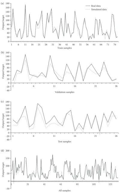
Fig. 3 compares the real and simulated values of FLAQ in the training, validation, test data set and all

data. A meaningful and distinctive agreement be-tween real and simulated values is illustrated in Fig 3. Considering the results of the different designed structure of ANNs, FLAQM with the higher value of R2_{, makes a more accurate correlation between} inputs and outputs. So, FLAQM, using 22 forest

Table 2. The performance measures of the best artificial neural networks in the test phase

Function

Structure Test set All data

activation training R2 _{MSE RMSE MAE R}2 _{MSE RMSE MAE}

Logsig-logsig-purelin LM 22-8-8-1 0.797 0.331 0.575 0.474 0.871 0.161 0.401 0.301

Logsig-purelin GDM 22-24-1 0.796 0.325 0.570 0.465 0.857 0.155 0.394 0.289 Tansig-tansig-purelin BFGS 22-14-14-1 0.817 0.342 0.585 0.489 0.813 0.148 0.385 0.276 Logsig-purelin CGB 22-14-1 0.757 0.315 0.561 0.451 0.848 0.152 0.390 0284 Tansig-tansig-purelin GDA 22-16-16-1 0.809 0.338 0.581 0.484 0.866 0.150 0.387 0.280 Tansig-tansig-purelin CGP 22-17-17-1 0.737 0.301 0.549 0.431 0.821 0.151 0.389 0.282 LM – Levenberg-Marquardt, GDM – gradient descent with momentum, BFGS – Broyden-Fletcher-Goldfarb-Shanno, CGB – conjugate gradient with Powell/Beale, GDA – gradient descent with adaptive learning rate, CGP – conjugate gradient with Polak/Ribière; optimum feed-forward neural network for the prediction of forest landscape aesthetic quality in bold; MSE – mean squared error, RMSE – root mean squared error, MAE – mean absolute error

Fig. 2. Scatter plots of output versus target forest landscape aesthetic quality values by artificial neural network: training data set (a), validation data set (b), test data set (c), all data (d)

(a) (b)

(c) (d)

-2.0 -1.5 -1.0 -0.5 0.0 0.5 1.0 1.5 2.0 2.5 3.0

-2.0 -1.5 -1.0 -0.5 0.0 0.5 1.0 1.5 2.0 2.5 3.0

-1.5 -1 -0.5 0 0.5 1 1.5 2 2.5 3 -1.5 -1 -0.5 0 0.5 1 1.5 2 2.5 3

O

ut

put

s

O

ut

put

s

Fig. 3. Real and simulated forest landscape aesthetic quality values by artificial neural network: training data set (a), validation data set (b), test data set (c), all data (d)

0 20 40 60 80 100 120 140 160 180

1 6 11 16 21 26 31 36 41 46 51 56 61 66 71 76

O

ut

pu

t/

ta

rg

et

Train samples

Real data Simulated data

-40 -20 0 20 40 60 80 100 120 140 160

1 6 11 16 21 26

O

ut

pu

t/

ta

rg

et

Validation samples

-40 -200 20 40 60 80 100 120 140 160 180

1 6 11 16 21 26

O

ut

pu

t/

ta

rg

et

Test samples

-50 0 50 100 150 200

1 21 41 61 81 101 121

O

ut

pu

t/

ta

rg

et

All samples

(a)

(b)

(c)

landscape characteristics, as model input variables, can be a more accurate model for the assessment of forest landscape aesthetic quality. Eqs. 7 and 8 are proposed as FLAQM in forest ecosystems:





_

_

1 exp net

j i i f Y Y T 

   (7)

where:

Ynet – sum of weighted inputs for PE_ki,

PE_ki – processing elements (PE) or neuron,

j – layer number,

i – neuron number,

T – threshold value.

















where:

LW_ji – layer weights,

IW_ji – input weights,

p_i – input signals,

∑b_i – biases.

The main application of FLAQM is to predict FLAQ based on landscape features. As an envi-ronmental decision support system tool, FLAQM is applied for decision-making on landscape man-agement in forest ecosystems to reduce the forest landscape degradation.

Sensitivity analysis of FLAQM

For the sensitivity analysis, each input variable was withdrawn while not manipulating any of the other variables and then the FLAQM was trained for every

pattern. According to results in Fig. 4, the share of each input variable of the developed FLAQM in de-sired output can be realized clearly. According to the sensitivity analysis, the values of livestock density, tree harvesting, virgin forest, animal grazing, and tree richness have been identified as the most signifi-cant variables which influence FLAQM (Fig. 4).

Considering trends in Figs 5a, d, livestock density and animal grazing in the landscape are negatively correlated with landscape aesthetic quality, so in the landscapes with cattle grazing activity the time con-sumption for recreation by visitors decreases. Con-sidering trends in Figs 5b, c, harvesting and virgin area land uses are correlated with aesthetic qual-ity of the landscape. The trend changes positively between harvesting and the spent time by visitors as aesthetic quality of the landscape increases. Ac-cording to Fig. 5c, virgin forest lands, belonging among the forest land uses, in particular, are posi-tively correlated with landscape aesthetic quality. Results point out to a high correlation between for-est landscape afor-esthetic quality and forfor-est land uses. According to Fig. 5e, tree richness, as one of the naturalness indicators, in particular, is positively correlated with landscape aesthetic quality. Results prove a positive correlation between landscape aes-thetic quality and tree richness in forest landscapes. The sensitivity analysis result is applied for the management of forest landscape aesthetic quality. LSU management, based on forest landscape char-acters with a higher value in the sensitivity analysis, helps managers to take a decision on forest proj-ect actions to protproj-ect the aesthetic quality of forest landscape and its benefits.

Fig. 4. Results of the sensitiv-ity analysis of forest land-scape aesthetic quality model (FLAQM) 0 5 10 15 20 25 30 35 40 Li ve stock density Harves tin g Virgi n fores t Animal grazi ng Tree richnes s River

view Slop

e Logs depo t Se a vi ew Settlements and Length of roa d Tre es dominant As pe ct Animal husbandry Trees dominant Ro cky hillside view Le ngth o f trail Canopy densi ty Trees abundance Te m pe rature Precipitat io n Altit ude Se nsiti vity of F LA Q M

Inputs of FLAQM

vil

lages view diame

te

r

DISCUSSION

Accordingly, our modelling approach combined a quantitative assessment of the aesthetic quality of for-est landscapes with a perception-based method to in-vestigate human perceptions of scenic beauty. FLAQM provides a framework for clearly analysing how objec-tive criteria of forest landscape will result in beholders’ preferences subjectively. The results of ANN model ling, especially its high accuracy (R2 _{= 0.871) in} com-parison with MLR results (R2 _{= 0.782), introduced} FLAQM as a comparative model for an assessment of forest landscape aesthetic quality. FLAQM was designed for forest managers or other decision-mak-ers and stakeholddecision-mak-ers to compare the LSUs in a forest ecosystem based on landscape quality and classify them for forest planning and support decisions.

The sensitivity of FLAQM recognized the tree rich-ness as one of the naturalrich-ness indicators, highly cor-related with landscape preferences. So, the

sustain-ability of forest landscape management depends on maintaining the landscape tree richness quality in a sustainable forest management project. Diversity in-dices and mainly the Shannon index is the most fre-quently used index in landscape quality assessment (Plexida et al. 2014). As we found, Dramstad et al. (2006) explored a positive correlation between land-scape preferences and Shannon index values. De La Fuente De Val and Mühlhauser (2014) proved a positive impact on visual quality in denser vegetation landscapes and a negative one in open vegetation landscapes. Vries et al. (2012) indicated that people preferred landscapes with natural structure and set-tings more than landscapes with human activities and impacts. Of all the variables, the sensitivity anal-ysis of FLAQM found a strong correlation between FLAQM output and forest land uses such as animal grazing, harvesting, and virgin forest. Animal grazing by local people and wood harvesting by government institutions are known as two main human activities

Fig. 5. Forest landscape aesthetic quality model (FLAQM) output for inputs variables: varied input livestock density (total number of individuals per hectare) (a), tree harvesting (b), virgin forest (c), animal grazing (d), tree richness (Shannon index) (e)

50 55 60 65 70

1.30 1.45 1.59 1.74

FL

A

Q

M

o

ut

pu

t

Tree richness

40 50 60 70 80

0.16 0.45 0.74 1.03

Harvesting

40 50 60 70

0.33 0.59 0.85 1.11

Animal grazing 50

55 60 65 70

0.01 0.26 0.52

FL

A

Q

M

o

ut

pu

t

Virgin forest 35

45 55 65 75 85

0.08 0.47 0.85 1.24

FL

A

Q

M

o

ut

put

Livestock density

(a) (b)

(c) (d)

in forest management and utilization in Hyrcanian forests. Considering results and human perceptions, we declare in LSUs where animal husbandry is lo-cated in landscape or the primary land use is wood harvesting or animal grazing, the forest landscape aesthetic quality decreases to not interesting land-scape. Carvalho-Ribeiro et al. (2013) declared that landscape physical components completely influence subjective landscape dimensions. As we found, they also suggested that land use would be taken as an es-sential asset for describing the landscape.

Our approach adopts a structured analysis of the aesthetic quality of forest landscapes, which is fos-tering the landscape quality protection. The results of research proved the capability of ANN in the quantification of forest landscape aesthetic qual-ity after forest project implementation. In this way, FLAQM, as an environmental decision support system in the hands of decision-makers, quantifies the landscape aesthetic quality of temperate broad-leaf forests in response to the forest project activi-ties and landscape structure, and it helps to find the most scenic LSUs for planning forestry activities.

Acknowledgement

We thank the manager of Kheirud Educational Forest at the University of Tehran for his valuable cooperation in the research process.

References

Boillereaux L., Cadet C., Le Bail A. (2003): Thermal properties estimation during thawing via real-time neural network learning. Journal of Food Engineering, 57: 17–23. Carvalho-Ribeiro S.M., Lovett A. (2011): Is an attractive forest

also considered well managed? Public preferences for forest cover and stand structure across a rural/urban gradient in northern Portugal. Forest Policy and Economics, 13: 46–54. Carvalho-Ribeiro S., Ramos I.L., Madeira L., Barroso F., Men-ezes H., Pinto Correia T. (2013): Is land cover an important asset for addressing the subjective landscape dimensions? Land Use Policy, 35: 50–60.

Chopra P., Sharma R.K., Kumar M. (2014): Regression models for the prediction of compressive strength of concrete with & without fly ash. International Journal of Latest Trends in Engineering and Technology, 3: 400–406.

De La Fuente De Val G., Mühlhauser S.H. (2014): Visual qual-ity: An examination of a South American Mediterranean

landscape, Andean foothills east of Santiago (Chile). Urban Forestry & Urban Greening, 13: 261–271.

de Vries S., De Groot M., Boers J. (2012): Eyesores in sight: Quantifying the impact of man-made elements on the scenic beauty of Dutch landscapes. Landscape and Urban Planning, 105: 118–127.

Dramstad W.E., Sundli Tveit M., Fjellstad W.J., Fry G.L.A. (2006): Relationships between visual landscape prefer-ences and map-based indicators of landscape structure. Landscape and Urban Planning, 78: 465–474.

Flott L.W. (2012): Using the scatter diagram tool to compare data, show relationship. Metal Finishing, 110: 33–35. Franco D., Franco D., Mannino I., Zanetto G. (2003): The

im-pact of agroforestry networks on scenic beauty estimation: The role of a landscape ecological network on a socio-cul-tural process. Landscape and Urban Planning, 62: 119–138. Groot J.C.J., Jellema A., Rossing A.H. (2010): Designing

a hedgerow network in a multifunctional agricultural landscape: Balancing trade-offs among ecological quality, landscape character and implementation costs. European Journal of Agronomy, 32: 112–119.

Intharathirat R., Abdul Salam P., Kumar S., Untong A. (2015): Forecasting of municipal solid waste quantity in a developing country using multivariate grey models. Waste Management, 39: 3–14.

Jahani A. (2019): Sycamore failure hazard classification model (SFHCM): An environmental decision support system (EDSS) in urban green spaces. International Journal of Environmental Science and Technology, 16: 955–964. Jahani A., Feghhi J., Makhdoum M.F., Omid M. (2016):

Op-timized forest degradation model (OFDM): An environ-mental decision support system for environenviron-mental impact assessment using an artificial neural network. Journal of Environmental Planning and Management, 59: 222–244. Nuruddin M.F., Ullah Khan S., Shafiq N., Ayub T. (2015):

Strength prediction models for PVA fiber-reinforced high-strength concrete. Journal of Materials in Civil Engineer-ing, 27: 2–16.

Plexida S.G., Sfougaris A.I., Ispikoudis I.P., Papanastasis V.P. (2014): Selecting landscape metrics as indicators of spatial heterogeneity – a comparison among Greek landscapes. International Journal of Applied Earth Observation and Geoinformation, 26: 26–35.

Ribe R.G. (2009): In-stand scenic beauty of variable retention harvests and mature forests in the U.S. Pacific Northwest: The effects of basal area, density, retention pattern and down wood. Journal of Environmental Management, 91: 245–260.